HAL Id: hal-00316971
https://hal.archives-ouvertes.fr/hal-00316971
Submitted on 1 Jan 2003
HAL is a multi-disciplinary open access
archive for the deposit and dissemination of
sci-entific research documents, whether they are
pub-lished or not. The documents may come from
teaching and research institutions in France or
abroad, or from public or private research centers.
L’archive ouverte pluridisciplinaire HAL, est
destinée au dépôt et à la diffusion de documents
scientifiques de niveau recherche, publiés ou non,
émanant des établissements d’enseignement et de
recherche français ou étrangers, des laboratoires
publics ou privés.
Adriatic Sea surface temperature and ocean colour
variability during the MFSPP
E. Böhm, V. Banzon, E. d’Acunzo, F. d’Ortenzio, R. Santoleri
To cite this version:
E. Böhm, V. Banzon, E. d’Acunzo, F. d’Ortenzio, R. Santoleri. Adriatic Sea surface temperature and
ocean colour variability during the MFSPP. Annales Geophysicae, European Geosciences Union, 2003,
21 (1), pp.137-149. �hal-00316971�
Geophysicae
Adriatic Sea surface temperature and ocean colour variability
during the MFSPP
E. B¨ohm1, V. Banzon2, E. D’Acunzo1, F. D’Ortenzio1, and R. Santoleri1
1Istituto di Scienze dell’Atmosfera e del Clima – CNR, Via Fosso del Cavaliere 100, 00133 Roma, Italy
2MPO/RSMAS, University of Miami, 4600 Rickenbacker Causeway, Miami FL 33149, USA
Received: 23 August 2001 – Revised: 6 August 2002 – Accepted: 3 September 2002
Abstract. Two years and six months of night-time Ad-vanced Very High Resolution Radiometer (AVHRR) sea sur-face temperature (SST) and daytime Sea viewing Wide Field of view Sensor (SeaWiFS) data collected during the MF-SPP have been used to examine spatial and temporal vari-ability of SST and chlorophyll (Chl) in the Adriatic Sea. Flows along the Albanian and the Italian coasts can be dis-tinguished year-round in the monthly averaged Chl but only in the colder months in the monthly averaged SST’s. The Chl monthly-averaged fields supply less information on cir-culation features away from coastal boundaries and where conditions are generally oligotrophic, except for the early spring bloom in the Southern Adriatic Gyre. To better char-acterise the year-to-year and seasonal variability, exploratory data analysis techniques, particularly the plotting of multi-ple Chl-SST histograms, are employed to make joint quan-titative use of monthly-averaged fields. Modal water mass (MW), corresponding to the Chl-SST pairs in the neighbour-hood of the maximum of each monthly histogram, are chosen to represent the temporal and spatial evolution of the preva-lent processes and their variability in the Adriatic Sea. Over an annual cycle, the MW followed a triangular path with the most pronounced seasonal and interannual variations in both Chl-SST properties and spatial distributions of the MW in the colder part of the year. The winter of 1999 is the colder
(by at least 0.5◦C) and most eutrophic (by 0.2 mg/m3). The
fall of the year 2000 is characterised by the lack of cooling in the month of November that was observed in the previ-ous year. In addition to characterising the MW, the two-dimensional histogram technique allows a distinction to be made between different months in terms of the spread of SST values at a given Chl concentration. During spring and sum-mer, the spread is minimal indicating surface homothermal conditions. In fall and winter, on the other hand, a spread of points suggesting a linear negative correlation between SST and Chl is found. This behaviour is related to the high
nutri-Correspondence to: E. B¨ohm
ent content of cooler water associated with upwelling or the Po River fresh water outflow.
Key words. Oceanography: general (diurnal, seasonal and
annual cycles; marginal and semienclosed seas; water masses)
1 Introduction
Circulation in the Adriatic Sea (Fig. 1) exhibits high spa-tial and temporal variability, involving several water masses (Artegiani et al., 1997a, b and references therein). Com-plicating factors include bottom topography, meteorological conditions and freshwater influx from rivers. To characterise interannual trends in water mass variability and associated flows, an extensive time series of detailed salinity and tem-perature data would be needed. Artegiani et al. (1997a, b) used 80 years of hydrographic data to infer general circula-tion, describe water mass structure and analyse air-sea in-teraction budgets in the Adriatic Sea. A cost and labour-efficient alternative would be to utilise satellite data, which are particularly suitable for this purpose because of the
syn-opticity and high spatial and temporal resolution. Even
though the satellite signal represents only surface processes, considerable insight into the underlying physics and biology can be obtained. The general tendency has been to use only a single sensor in previous satellite studies of the Adriatic Sea. The combined use of different satellite sensors would permit identification of features year-round that may not be detected by a single sensor. At present, the two most com-mon satellite-derived parameters for which surface maps are readily available are sea surface temperature and chlorophyll. However, temperature exhibits conservative behaviour, while chlorophyll does not. Thus, the combined use of SST and Chl needs to be explored. The Adriatic Sea provides an interest-ing test site because of its complex circulation. Usinterest-ing these ideas, this study examines spatial and temporal variability of SST and Chl in the Adriatic Sea during the field
observa-138 E. B¨ohm et al.: Adriatic Sea surface temperature and ocean colour variability
44N
42N
40N
14E 16E 18E
Ancona Gargano Po Alb ania O tra nto Sill Dalm atian C oast Pom o Pit
Fig. 1. Bathymetric chart of the Adriatic Sea (depth in meters) with named places cited into the text.
tional period of the Mediterranean Forecasting System Pilot Project (MFSPP).
The physical characteristics of the Adriatic basin affect its circulation; it is almost completely surrounded by land, communicating with the Ionian Sea only at its southern-most extreme (Fig. 1). Corresponding to the changes in the bathymetry of the basin, three subregions are usually recog-nised. The north Adriatic averages less than 50 m in depth and gradually deepens towards the central Adriatic (average depth ∼100 m). In the central area, a shallow depression of about 250 m is known as the Jabuka or Pomo Pit, or Mid-Adriatic Depression. A relatively shallow sill demarcates the beginning of the southern Adriatic which contains a large de-pression of >1000 m depth. The Otranto sill (800 m) is found at the southern end of the basin.
Recent climatological analysis of several hydrographic datasets show that the general surface flow in the Adriatic Sea is cyclonic with three embedded gyres (Artegiani et al., 1997b). Interaction with the bottom and lateral borders also results in the formation of smaller gyres, eddies, and other smaller scale features such as filaments (Borzelli et al., 1999). The entrance flow occurs on the eastern side of the Straits of Otranto and brings in water from the oligotrophic Ionian Sea. Part of the surface flow then follows the Dal-matian coast as the Eastern Adriatic Current. At the north-ernmost end of the basin, the coastal flow is referred to as the Northern Adriatic Current until the Po River plume is encountered. Mixing with fresher water from the Po and
adjacent rivers results in entrainment and major water mass modification (Hopkins et al., 1999). Downstream of the mix-ing area, a well-defined Western Adriatic Current becomes organised, and continues along the Italian coast, exiting on the western side of the Straits of Otranto. Along the cen-tral axis of the basin are three principal gyres associated with the Adriatic subregions. These are the Northern, Mid- and Southern Adriatic gyres. In addition, episodes of dense water formation occur in the northern and southern Adriatic under particular wintertime conditions with possible influences on the surface circulation (Artegiani et al., 1997a, b; Hopkins et al., 1999). The sinking of dense water requires replacement flow at the surface and may result in greater penetration of an adjacent water mass (Hopkins et al., 1999).
The Adriatic Sea is one of the highly productive areas in the Mediterranean basin. Yet, the spring bloom is not well described despite its obvious importance to fisheries and re-source management. Estimates based on the Coastal Zone Color Scanner (CZCS) by Antoine et al. (1995) confirm that the Adriatic Sea has the highest pigment biomass and pri-mary production of all the Mediterranean sub-basins. Us-ing CZCS data, Barale et al. (1986) showed a direct cor-relation between the winter-spring pigment distributions in the northern Adriatic and the Po River freshwater discharge. Barale et al. (1986) also noted that wintertime vertical mix-ing over the northern shelf could be important because of the co-occurrence of high pigment levels with meteorologi-cal conditions associated with dense water formation. Using a few CZCS images, Barale et al. (1984) examined the cor-respondence between large-scale circulation features in the Adriatic Sea and the spatial patterns in apparent temperature and attenuation coefficient maps. Because the interaction of coastal flow and river runoff with Adriatic water masses is clearly visible in the CZCS images, they concluded that the coastal water parameters are a natural tracer of the surface circulation.
The Sea-viewing Wide Field of view Sensor (SeaWiFS) data used in this study offer superior spectral and temporal resolution than CZCS and coverage. Using such data re-cently, Banzon et al. (private communication), investigated the year-to-year variability in the timing, duration and spa-tial extent of the surface phytoplankton bloom in the south-ern Adriatic Sea and related them to restratification conse-quent to deep water formation occurring in the South Adri-atic Gyre.
The remotely sensed SST field in the Adriatic Sea has been investigated using AVHRR data. Gacic et al. (1997) analysed the seasonal and interannual variability of the Adriatic based on monthly, 18-km resolution SST data alone. They found a strong interannual variability in the basin-wide mean SST and a general correspondence between thermal and oceano-graphic features in the Adriatic Sea. Low horizontal resolu-tion and the reduced thermal contrast in the summer strongly limited their analysis. The addition of ocean colour informa-tion to SST fields offers for the first time an opportunity to monitor circulation year round, and not only when thermal contrast is sufficiently strong.
140 E. B¨ohm et al.: Adriatic Sea surface temperature and ocean colour variability
In this paper, after a description of the dataset (Sect. 2), we analyse both SST (Sect. 3.1) and ocean colour (Sect. 3.2) patterns and relate them to the known features of the circu-lation (Sect. 3.3). Moreover, we introduce the Modal water mass (MW), defined on the basis of joint SST and Chl prop-erties, as a statistical graphical tool to describe interannual and seasonal variations at the basin level (Sect. 3.4). The aim is to develop a prototype methodology that can be applied elsewhere and is sensitive to long-term changes.
2 The Dataset
2.1 SST data processing
AVHRR data from the NOAA-14 satellite were col-lected by the HRPT receiving station at Istituto di Fisica dell’Atmosfera (IFA) in Rome, Italy. The daily SST maps for the Eastern Mediterranean were produced by IFA for the MFSPP project in real-time for the model-data assimilation. About 1000 night-time passes covering the Eastern Mediter-ranean were received for the period extending from 1 January 1999 to 31 December 2000. The data were processed us-ing the DSP software developed at the University of Miami to obtain 2-channel algorithm (McClain et al., 1985) SSTs. Exclusion of cloud-contaminated pixels is necessary when dealing with time series of AVHRR imagery. Cloud detec-tion was performed automatically, then quality control was done manually to eliminate residual contaminated pixels. Ar-eas with clouds were successively flagged as bad data. Data over the Eastern Mediterranean were remapped in equirect-angular projection at full resolution. For this paper, data for
the Adriatic Sea (39.5–46.5◦N, 12.0–20.0◦E) were extracted
from the original MFSPP maps and remapped on a 512 by 600 pixel grid at a 1 km resolution using an equirectangular projection.
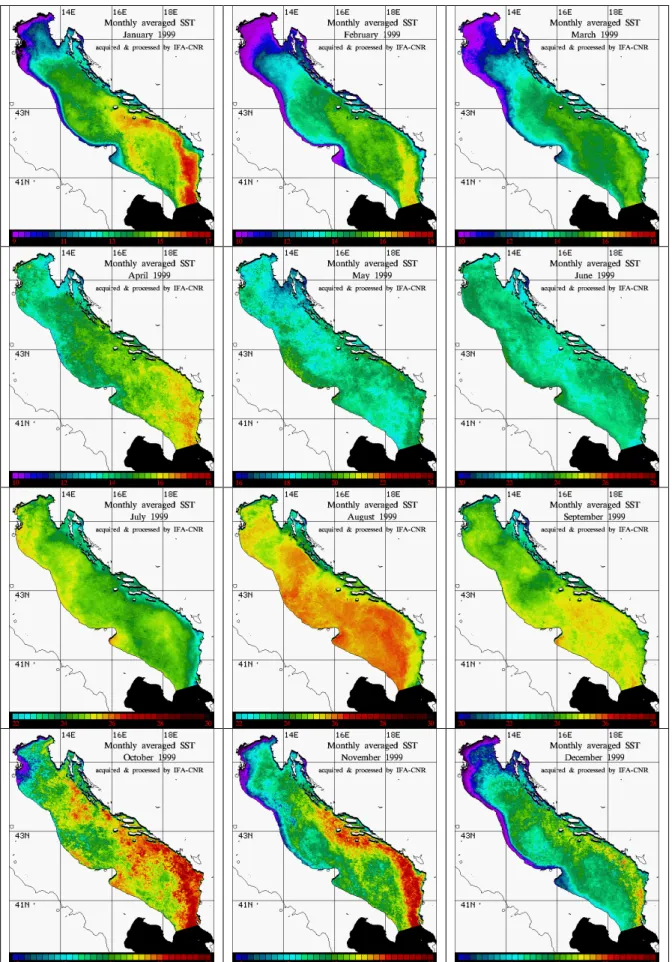
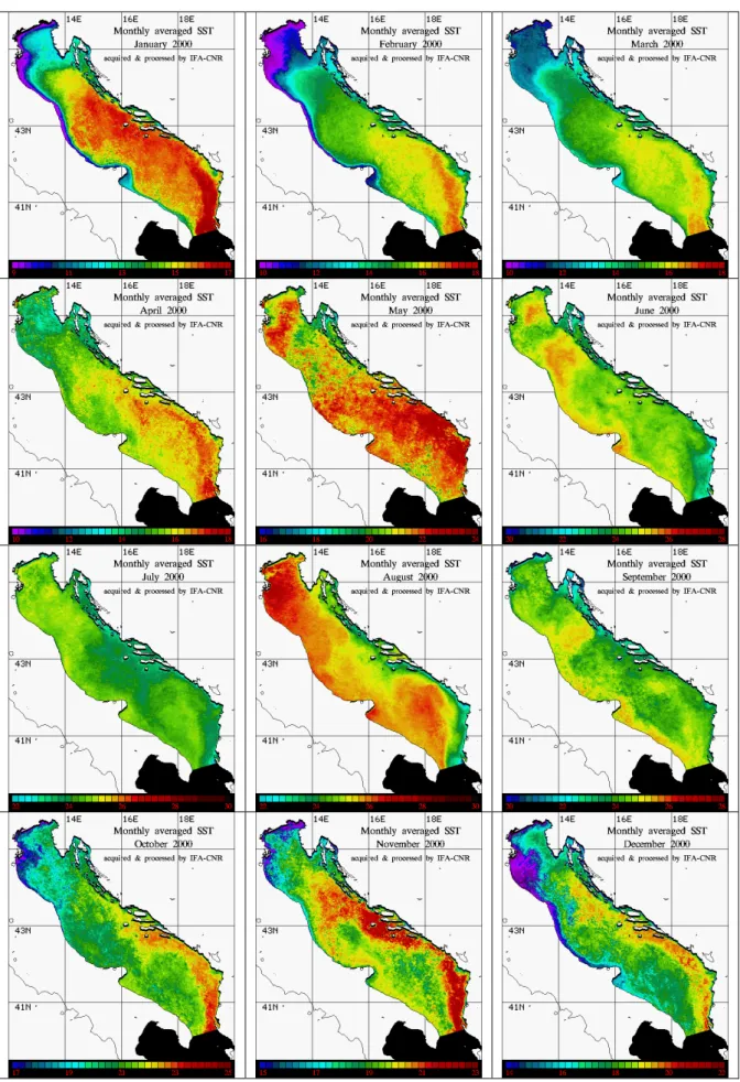
From the daily maps, monthly SST fields were constructed from January 1999 to December 2000 (Fig. 2a, b). The in-dividual fields produced for the MFSPP often had an insuffi-cient number of observations hindering the computation of a meaningful monthly field. In fact, some pixels were always flagged as cloudy due to the tendency of automated cloud detection to exclude cold coastal current pixels that are im-portant to the present analysis. In order to preserve informa-tion for the coastal areas and reduce the effect of outliers (i.e. clouds) in the calculation of monthly SST fields, monthly median maps were used instead of monthly averaged maps. The median operator has the advantage of excluding pixels that are cloud contaminated as well as those affected by in-strumental noise.
2.2 SeaWiFS data processing
To supplement the information obtained from the MFSPP SST, we used SeaWiFS ocean colour data for the same pe-riod. The Global Area Coverage (GAC) Level 2 data at 4-km resolution were obtained from NASA. The standard
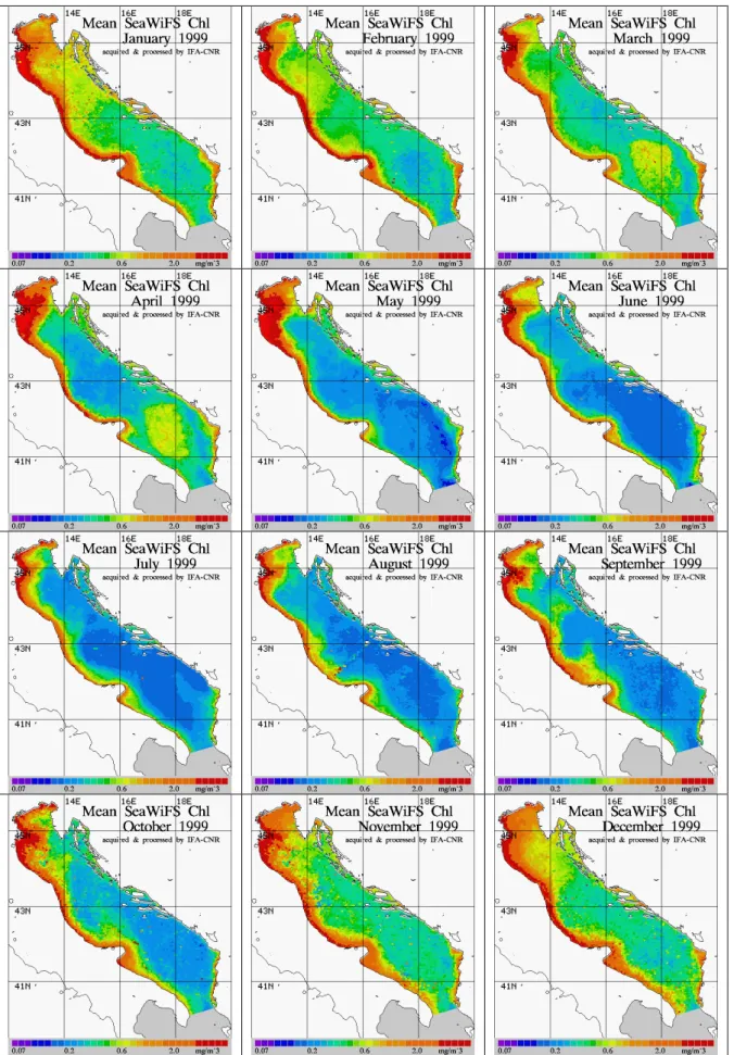
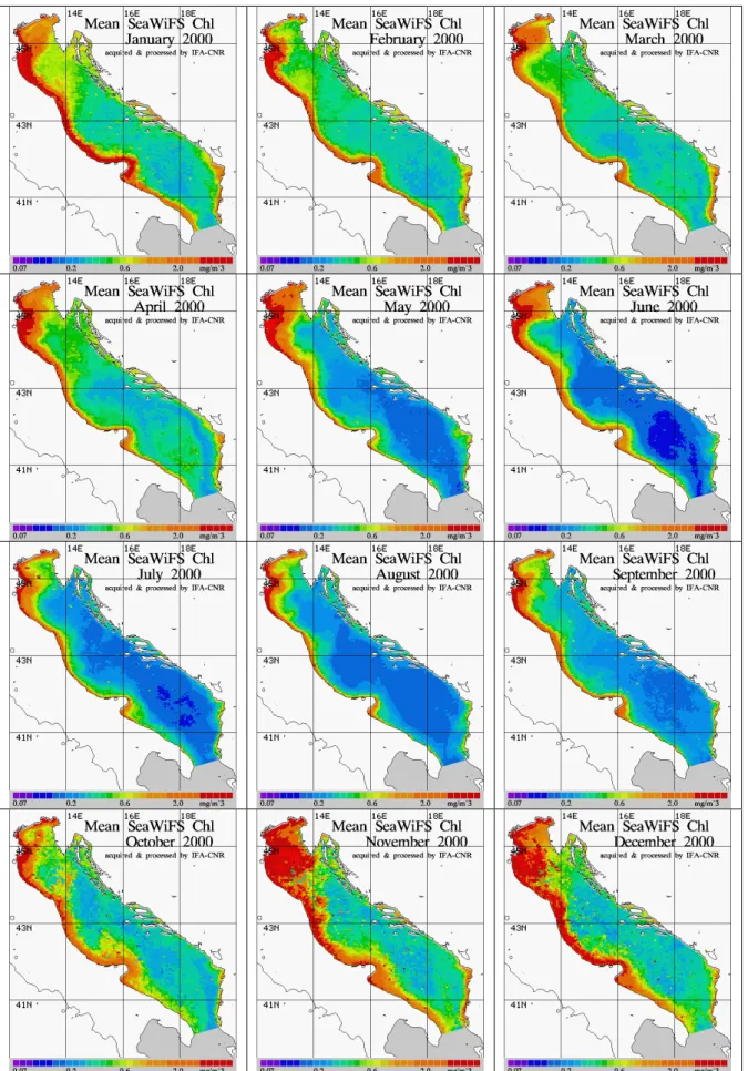
NASA GAC processing is performed using the dark pixel at-mospheric correction and the OC-4v4 bio-optical algorithm (O’Reilly et al., 2000). The use of GAC ocean colour data is justified by the focus of the present paper on the basin-scale features and not on small-scale details. A series of masks and flags are computed and stored in an additional product (L2-flags) in order to let the end-user verify if any contamination of the final data has occurred. A detailed description of the data processing is given by Patt et al. (2000). For the Adri-atic Sea, we extracted the chlorophyll data and the associated flags, remapping them to the same projection and resolution as the SST fields. Then, computing the average chlorophyll for each pixel yielded monthly maps (Figs. 3a and b).
In our case, we decided not to apply the Case 2 and shal-low water masks to the chlorophyll maps. This choice was dictated by a preliminary analysis showing that the applica-tion of SeaWiFS masks to maps of the Adriatic Sea tends to eliminate some important circulation features. In particu-lar, application of the Case 2 water and shallow water masks leads to the masking of the whole northern part of the basin and the Italian coastal region. This leads to a discrepancy in the coverage between SST (unaffected by shallow and Case 2 water) and Chl fields that is restrictive for a basin-wide anal-ysis. The above choice renders our results more complete since we are primarily interested in the pattern of the circu-lation features traced by the chlorophyll fields at the monthly scale. Thus, our focus is mainly on the horizontal gradients rather than on the absolute values of chlorophyll. In any case, the reader should bear in mind the limitations of the defini-tion of “Chlorophyll” as used in this paper, i.e. there might be a difference between the estimated chlorophyll for the Sea-WiFS maps and in situ values.
2.3 Modal water analysis
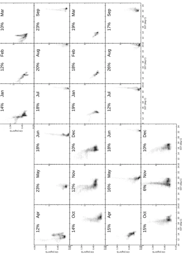
The MW approach is a variant of the exploratory data anal-ysis (EDA) approach. It relates to the relative pattern rather than the absolute value of the data and focuses on the most populated cluster in Chl-SST space. MW is defined as the most common Chl-SST pair (i.e. the mode or maximum fre-quency) in the 2-D histogram constructed with the digital counts of all non-land pixels associated with each monthly mean Chl-SST image pair (Fig. 4a shows all the SST median maps with white flagged MW and Fig. 5 shows the 2-year-long MW time series obtained connecting all the monthly values). For each 2-D histogram, MW is identified by se-lecting data within a 9 × 9 count box centred on the mode value, with a frequency greater than 30% of the modal fre-quency. This box size and frequency threshold is a compro-mise which satisfies the necessary prerequisites of: (a) hav-ing enough pixels flagged as MW; (b) retainhav-ing the Chl-SST selectivity i.e. avoiding including pixels that are not MW. The points that satisfy the criteria are then highlighted (in white) on the monthly median SST images (Fig. 4a). The individual monthly histograms are shown in Fig. 4b.
Consequently, the MW represents the water mass charac-terised by the joint Chl-SST pairing that occurs most
fre-142 E. B¨ohm et al.: Adriatic Sea surface temperature and ocean colour variability
144 E. B¨ohm et al.: Adriatic Sea surface temperature and ocean colour variability
Fig. 4a. Spatial distribution of modal pixels for the period January 1999 -
De-cember 2000. Each row, except for
the first and last contains 6 months (i.e. two consecutive seasons) of the MW distribution (in white) plotted over the monthly median SST image.
quently in the basin during the selected month. The tem-poral variability in the spatial MW distribution illustrates the prevailing mode of variability at the basin scale. Indepen-dent of the physical and biological processes involved in its formation, MW effectively combines the information of the individual monthly SST and Chl fields. As will be evident in the discussion of the results, the MW does not reach the Italian coastal and northern parts of the Adriatic Sea and is composed, therefore, of “actual” rather than “apparent” Chl values. Thus, the non-application of Case 2 and shallow-water flags discussed in Sect. 2.2 is not critical to the present analysis.
3 Results and discussion
We discuss in Sect. 3.1 the features visible in the monthly median SST maps, in Sect. 3.2 the features detected in the monthly mean Chlorophyll maps, in Sect. 3.3 the combined Chl-SST characteristics and finally, in Sect. 3.4, we apply the MW analysis to diagnose the prevailing state of the Adriatic Sea.
3.1 Sea surface temperature
Temperature data have been shown to be good indicators of the circulation in the Adriatic Sea in winter when thermal contrast is strong between water masses (Gacic et al., 1997).
In general, the SST values in winter-spring 1999 were the coldest and became progressively warmer over the next 2 years (Fig. 2a). The wintertime SST difference between 2000
and 1999 is greater than 2◦C in January in the central and
southern Adriatic Sea, where ∼80% of Adriatic dense water originates (Artegiani et al., 1997b). Over the northern shelf (where the rest of the Adriatic dense water is formed) SST
reaches its maximum difference (2◦C) between 1999 and
2000 in March. Heat loss is associated with the presence of the Bora, a cold, dry wind that cools the surface waters lead-ing to deep water formation in the northern Adriatic. In the southern Adriatic Gyre, Banzon et al. (private communica-tion) estimated large heat losses in 1999 and 2000 that could drive deep convection to about 500 m, as observed in the rel-evant MFSPP XBT sections (Civitarese and Gacic, 2001).
During the winter months, the northern Adriatic shelf wa-ters are cooler than the rest of the basin; the lowest tempera-tures are associated with the Po River outflow coastal flows. During the spring months, circulation features in the northern Adriatic are difficult to discern except for the slightly warmer water near the Po outflow. In autumn, the cooler coastal flows become visible. The Western Adriatic Current is visible as a very cold coastal vein in the SST maps from November to March.
In the Middle Adriatic, the coastal upwelling causes cooler temperatures off the Dalmatian coast in July and August
de-10 12 14 16 18 20 22 24 0.15 0.45 1.34 4.00 Chl (mg/m^3) Jan 14% 10 12 14 16 18 20 22 24 1 Feb 12% 10 12 14 16 18 20 22 24 1 Mar 10% 10 12 14 16 18 20 22 24 0.15 0.45 1.34 4.00 Chl (mg/m^3) Apr 12% 10 12 14 16 18 20 22 24 1 May 23% 10 12 14 16 18 20 22 24 1 Jun 18% 10 12 14 16 18 20 22 24 1 Jul 18% 10 12 14 16 18 20 22 24 1 Aug 20% 10 12 14 16 18 20 22 24 1 Sep 23% 10 12 14 16 18 20 22 24 0.15 0.45 1.34 4.00 Chl (mg/m^3) Oct 14% 10 12 14 16 18 20 22 24 1 Nov 12% 10 12 14 16 18 20 22 24 1 Dec 10% 10 12 14 16 18 20 22 24 1 Jan 19% 10 12 14 16 18 20 22 24 1 Feb 18% 10 12 14 16 18 20 22 24 1 Mar 19% 10 12 14 16 18 20 22 24 0.15 0.45 1.34 4.00 Chl (mg/m^3) Apr 15% 10 12 14 16 18 20 22 24 1 May 16% 10 12 14 16 18 20 22 24 1 Jun 18% 10 12 14 16 18 20 22 24 SST (deg C) 1 Jul 12% 10 12 14 16 18 20 22 24 SST (deg C) 1 Aug 26% 10 12 14 16 18 20 22 24 SST (deg C) 1 Sep 17% 10 12 14 16 18 20 22 24 SST (deg C) 0.15 0.45 1.34 4.00 Chl (mg/m^3) Oct 15% 10 12 14 16 18 20 22 24 SST (deg C) 1 Nov 6% 10 12 14 16 18 20 22 24 SST (deg C) 1 Dec 10%
Fig. 4b. Chl-SST histograms for the same months shown in Fig. 4a. For each month the surface area occupied by MW is indicated as percent of the total.
146 E. B¨ohm et al.: Adriatic Sea surface temperature and ocean colour variability
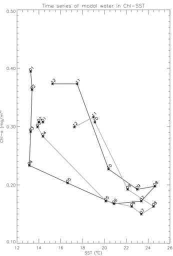
Fig. 5. Modal water time series. This plot illustrates the seasonal and interannual progression of the MW in the Chl-SST domain. It is obtained by connecting the maxima (in frequency) of each Chl-SST monthly histogram. The numeric labels, in the format YYMM indicate year and month from which they were obtained. The darker (lighter) line is for the year 1999 (2000). Wintertime warmer SST and lower Chl are observed in 1999 relative to 2000.
scribed by Borzelli et al. (1999), propagate offshore to the basin centre and exhibit high spatial-temporal variability re-sulting in a wide band of cooler water in the median SST field (Figs. 2a and b).
In the southern Adriatic, the most distinct thermal features are the cold Western Adriatic Current and, on the opposite coast, the Ionian Sea inflow into the South Adriatic Gyre. The Ionian Sea water is visible as a warm intrusion in the autumn-winter period and as a cold vein in summer. The Ionian Inflow continues northward along the coast and is clearly visible up to the Istrian peninsula (e.g. August 1999 and 2000).
3.2 Chlorophyll concentrations
The maps of monthly averages (Fig. 3a and b) show that high chlorophyll concentrations are always present in the north-ern Adriatic sub-region, where the outflow of many North-ern Italian rivers is found. The highest values coincide with
the Po River plume and the associated exiting coastal flow, known as the Western Adriatic Current. This current flows along the Italian coast and is observable year round but its offshore extension varies. From May to August, the Western Adriatic Current Chl signature vanishes south of the Gargano peninsula because the flow is weaker in this period. Evidence of filaments coming off this current can be found, especially in winter north of Ancona and at the tip of the Gargano penin-sula. These observations are in agreement with previous work in the Adriatic using CZCS data (Barale et al., 1986, 1984).
In summer (e.g. June–September 1999, July–October
2000), the protruding cross-basin feature associated with the Po river plume can be distinguished from the high-chlorophyll area along the northern Italian coast. The distinc-tion between the Po river plume and the Northern Adriatic Current is obscured when the water column begins to mix in late autumn but reappears when the water column heats up and thus stabilises towards summer. This distinct pattern is also observed briefly in spring: February–March 1999 and March–April 2000.
In the deeper area of the northern Adriatic, Chl concen-trations tend to be lower than the coastal flows but are still greater than in the southern Adriatic, excluding the spring
bloom period. Another salient circulation feature in the
northern sub-basin is a maximum north of Ancona which seems to extend offshore from the Western Adriatic Current, possibly due to the interaction between the circulation in the northern and in the middle Adriatic. This feature is most vis-ible in the winter of both years.
In the central Adriatic, the only manifestation of the Mid-Adriatic Gyre is slightly more oligotrophic water than the background in the summer of both years. From June to Au-gust, the oligotrophic patch in the central Adriatic appears to be coupled with a larger one to the south.
To the south, the South Adriatic Gyre and the two coastal currents on its flanks are easily recognised in the monthly maps. The most remarkable feature is the spring bloom in the gyre centre. In 1999, the bloom becomes evident in March– April and extends over most of the southern Adriatic. In 2000, the bloom is much weaker and is visible only along the southern boundary of the gyre in April. An extensive analysis of this bloom and its correlation with restratifica-tion following deep water formarestratifica-tion is discussed in Banzon et al. (private communication). The rest of the year, Chl val-ues in the gyre are minimal. High Chl concentrations along the Albanian Coast are indicative of the South Adriatic Cur-rent.
3.3 Combined Chl-SST features
In the Chl fields, derived from ocean colour observations down to the first optical depth as opposed to the skin layer temperature measured by the SST, filaments are fairly well visible and complement the information provided by the SST fields. Deep water formation events were expected to be eas-ily inferred from the SST median maps but the phenomenon
occurs on a scale of days and the associated cooling of sur-face waters is probably less evident in monthly median SST fields. Even though, for a few days in winter 1999 and 2000, SSTs were lower than the characteristic value of the Southern
Adriatic deep water mass (<13◦C), this is not indicated in the
monthly median SST (or monthly mean not shown) of 2000. In any case, dense water formation is a complex process that requires, among other things, a long pre-conditioning period of heat loss and salt gain that clearly is not taken into ac-count by our analysis. Deep convective mixing associated with dense water formation brings up nutrients into the eu-photic zone. These nutrients are critical to the Chl bloom later in the warming season (observed in 1999 and to a lesser degree in 2000), a topic examined in detail elsewhere (Ban-zon et al., private communication).
The winter-spring coastal vein of cold waters along the Italian coast is narrower relative to the high chlorophyll area and coincides only where chlorophyll is highest. Filaments and small eddies coming off the western current are clearly visible in the chlorophyll data (Fig. 3a) but their offshore propagation is less obvious in the SST field (e.g. February 1999, Fig. 2a). Indeed, mixing of the filament water with ambient water rapidly homogenises the SST field. Instead, the surface Chl signal persists because phytoplankton con-tinue to reproduce until nutrients are exhausted; also, time is required for phytoplankton injected into the oligotrophic offshore, areas to be diluted by the mixing with low nutrient water and/or to be grazed by zooplankton. It should be noted that the Western Adriatic current is particularly rich since it exports about half of the total nutrient inputs into the north-ern Adriatic including contributions from the Po River (De-Gobbis and Gilmartin, 1990). Offshore to the Western Adri-atic Current, the thermal gradients become negligible due to winter surface homothermal conditions. Coastal filaments are spatially variable and narrow so that averaging tends to weaken the signal. In summer, the spatial coherence between the SST and chlorophyll maps is diminished because of low temperature contrast. With the exception of April 2000 the Ionian Inflow is less evident in the chlorophyll maps while the centre of the gyre stands out when a large spring bloom occurs (e.g. March–April 1999).
3.4 Modal water patterns
Three aspects of the MW in the course of the 2-year study period are treated in this section. The first is the spatial dis-tribution of the MW (flagged in white in Fig. 4a); the second is the Chl-SST histogram shape (Fig. 4b) to place the MW in the context of the basin-wide Chl-SST characteristics; the third is the MW temporal trajectory in the Chl-SST space (Fig. 5).
The MW progression over the entire 2 years from January 1999 to December 2000 is shown in Fig. 4a. Odd rows show the cooling (1999, 1999–2000, and 2000) and even rows the warming (1999 and 2000) half of each yearly cycle, respec-tively. During the cooling, the colours in the SST fields go from green to blue, and during the warming, from blue
to red, according to the colour scale used in Fig. 2. The distribution of the MW is shown in white in Fig. 4a to try and identify the associated Adriatic water masses. In win-ter 1999, MW is found between incoming Ionian wawin-ter and Chlorophyll depleted South Adriatic Gyre waters (January– February) to then become the incoming Ionian water mass (March). In spring 1999 MW initially (April) found in the central Adriatic spreads to the southern (May) and accumu-lates in the southern Adriatic (June). In summer 1999, MW present in the central part of the southern basin spreads to the oligotrophic northern and southern basins. In the fall 1999, MW remains in the transition region between the Ionian and the central waters of the Adriatic Sea. In winter 2000, MW is initially found in the central and southern basins with the ex-clusion of the inflowing Ionian water (January), then it fills a greater portion of the southern basin (February), and fi-nally occupies the southern Adriatic and part of central Adri-atic (March). In spring 2000, MW becomes oligotrophic by extending its area of influence from the central (March) to the southern basin (April). In summer 2000, MW is present in June in the southern basin, reaching its maximum north-ward extension in July and then retreats in August. In the fall 2000, MW is found in the transitional central and south-ern basins (October), and then within the inflowing Ionian current (November and December).
The seasonal evolution indicates that MW is spatially scat-tered during fall with a notable exception in December 2000 when MW is clearly associated with the inflow of Ionian water along the Dalmatian coast. MW coalesces in winter within transitional water masses that have Chl-SST charac-teristics intermediate between the inflowing Ionian waters and the resident Adriatic waters. The extent of the area oc-cupied by MW (also shown as % in Fig. 4b) is highly depen-dent on the presence (low)/absence (high) of a chlorophyll bloom. The fact that surface waters where a bloom is occur-ring are not classified as MW is due to the high Chl gradients present in a patchy field such as that where a bloom is found. MW pixels in spring (1999 and 2000) expand from mid-basin to the southern basin as they take part in the horizontal wa-ter mass homogenisation typical of this period. No major change in MW distribution is detected in summer when it occupies both the Central and the Southern Adriatic Seas.
The patterns revealed by the MW distribution are consis-tent with the known major circulation features in the olig-otrophic portion of the Adriatic Sea. The MW spatial dis-tribution recognises the following three hydrographic condi-tions:
1. Incoming water masses such as those entering along the Albanian coast in fall (2000) and winter (1999) and flanking the previously discussed South Adriatic Gyre, 2. Water masses such as the transition waters between
am-bient Adriatic and newly supplied Ionian water, 3. Spreading homothermal and oligotrophic waters in
148 E. B¨ohm et al.: Adriatic Sea surface temperature and ocean colour variability A more detailed look at the qualitative relationship
be-tween modal water and the rest of the water masses present in the basin is afforded by Fig. 4b where a darker grey indicates a higher frequency. The quantitative range in MW surface area is between 6% and 26% of the total area in November and August 2000, respectively.
The month-by-month shape of the histograms is very simi-lar in the autumn of 1999 and 2000 when the maximum range in SST values is observed in the Adriatic Sea, as is the per-cent of surface area occupied by MW (except for November). On the contrary, the minimum range in properties is observed in summer when minimum Chl and maximum SST values are found. In winter and spring, the range in Chl-SST prop-erties is intermediate with respect to the other two seasons. In addition to the seasonal changes, the light grey tails of the histograms at higher than MW Chl concentration are occu-pied by the coastal waters of the Western Adriatic Current, the bloom waters and the Albanian coastal waters. A more detailed analysis of the shape of the histogram is tempting but is beyond the scope of this work that focuses on the prevalent water mass in each monthly interval and excludes interesting, but much more complex, coastal phenomena.
The temporal changes in the MW characteristics, in view of what has been discussed above, are summarised in a di-agram (Fig. 5). The MW trajectory roughly traces a trian-gle with one extreme on the lower right (high SST, low Chl) and the other on the top left (high Chl, low SST). The tran-sition during the autumn is linear from August to Decem-ber, showing cooling and an increase in Chl. The winter-spring-summer transition occurs in 2 steps: first chlorophyll decreases while SST remains roughly constant (December to April), then from April to August, SST increases while Chl
is almost constant below 0.2 mg/m3.
In the absence of interannual variability, one would expect the seasonal cycle to repeat with cold high-chlorophyll wa-ters in winter and warm low-chlorophyll wawa-ters more likely in summer. However, significant MW interannual variability is observed. While the modal classification detects the Chl-SST pairing occurring most frequently each month, the abso-lute values of these defining properties are not fixed. There-fore, part of the variability observed in the modal time series plot is caused by different water masses that in turn are MW. The spatial distribution of modal water is fundamental in in-dicating the processes that make it stand out. For example, the absence of modal water in the north confirms the decou-pling between the northern Adriatic and the rest of the basin from the biological and thermal points of view.
4 Conclusions
The combined use of SST and Chl permits the identifica-tion of circulaidentifica-tion features and gives insight into basin dy-namics over a 24-month period. Flow along the Albanian and Italian coasts (the North Adriatic Current and Western Adriatic Current, respectively) can be distinguished year-round in the SeaWiFS chlorophyll maps but is discernible
only in the colder months in the corresponding SST im-ages. Ocean colour data give less resolution of circulation features in the basin interior where conditions are generally oligotrophic except for the winter-spring bloom in the south Adriatic gyre. The upwelling and filament-formation off the Dalmatian coast in July–August, evident in SST maps, is not associated with high chlorophyll concentrations. In the southern basin, the SST field is a better indicator of the Io-nian inflow while the chlorophyll field shows the interior of the South Adriatic Gyre especially during the spring bloom. A year-to-year difference was evident in both the SST and the chlorophyll monthly maps, but no simple direct relation was found. The winter–spring 1999 was unusually cold, coincid-ing with high biological production in the Adriatic, particu-larly in the northern and southern sub-basins. The follow-ing winter-sprfollow-ing was warmer and not as productive. This leads to the expectation that temperature is inversely corre-lated with chlorophyll because the nutrients are supplied by upwelling colder underlying water. However, MFSPP XBT sections in the area of the South Adriatic gyre showed that deep convection occurred in 2000 but not in 2001. This sug-gests that factors other than temperature (such as the timing of convection and grazing pressure) may be critical in de-termining deep convection and related increased production (Banzon et al., private communication).
Use of the MW Chl-SST characteristics and spatial distri-butions in the Adriatic Sea illustrates quantitatively the sea-sonal and interannual variability during the MFSPP observa-tional period in the basin. The MW annual cycle is roughly triangular and illustrates a three-stage transition among the states of the Adriatic Sea system. The first half of the cool-ing season exhibits coolcool-ing and increascool-ing chlorophyll con-centration while the second half exhibits mainly a decrease in chlorophyll and slight cooling. During the seasonal warm-ing, the SST and Chl roles are reversed and the heating of the MW is accompanied by a slight decrease in Chl concen-tration. A decrease in the summertime chlorophyll minimum and an increase in the wintertime SST minimum indicate a MW change toward warmer and less productive waters over the 1999–2000 period. The spatial distribution of MW in-dicates to some extent the degree of homogeneity that en-sues from the presence of external forcing. In the absence of forcing (relaxation), the surface area of MW increases (sum-mertime warming and de-eutrophication). The causes of the observed patterns are to be sought in meteorological forcing and its climatological evolution but go beyond the scope of the present paper.
Acknowledgements. This work was primarily funded by the Italian
Space Agency (ASI) under contract ARS0021. The work was done as part of the MFSPP Project, funded by the European Commission. The authors would like to thank the SeaWiFS Project (Code 970.2) and the Distributed Active Archive Centre (Code 902), at Goddard Space Flight Centre, Greenbelt, MD 20771, for the production and distribution of these data, respectively. NASA’s Mission to Planet Earth Program sponsors the above activities. The authors would also like to thank the first anonymous reviewer for his comments that have helped make significant improvements to the paper.
Topical Editor N. Pinardi thanks two referees for their help in evaluating this paper.
References
Antoine D., Mor´el, A., and Andr´e, J.-M.: Algal pigment distribu-tion and primary producdistribu-tion in the eastern Mediterranean as de-rived from coastal zone colour scanner observations, J. Geophys. Res., 100, 16 193–16 209, 1995.
Artegiani, A., Bregant, D., Paschini, E., Pinardi, N., Raicich, F., and Russo, A.: The Adriatic Sea general circulation: Part I: Air-Sea Interactions and water mass structure, J. Physical Oceanography, 27, 1492–1514, 1997a.
Artegiani, A., Bregant, D., Paschini, E., Pinardi, N., Raicich, F., and Russo, A.: The Adriatic Sea general circulation: Part I: Baro-clinic circulation structure, J. Physical Oceanography, 27, 1515– 1532, 1997b.
Barale, V., McClain, C. R., and Malanotte-Rizzoli, P.: Space and time variability of the surface colour field in the Northern Adri-atic Sea, J. Geophys. Res., 91, 12 957–12 974, 1986.
Barale, V., Malanotte-Rizzoli, P., and Hendershott, M. C.: Re-motely sensing the surface dynamics of the Adriatic Sea, Deep Sea Res., 31, 1433–1459, 1984.
Borzelli, G., Manzella, G., Marullo, S., and Santoleri, R.: Oberva-tions of coastal filaments in the Adriatic Sea, J. Marine Systems, 20, 187–203, 1999.
Civitarese, G. and Gacic, M.: Had the Eastern Mediterranean tran-sient an impact on the new production in the south Adriatic?, Geophys. Res. Lett., 28, 1627–1630, 2001.
Degobbis, D. and Gilmartin, M.: Nitrogen, phosphorus, and bio-genic silicon budgets for the northern Adriaitc Sea. Oceanol. Acta, 13, 31–45, 1990.
Gacic, M., Marullo, S., Santoleri, R., and Bergamasco, A.: Analysis of the seasonal and interannual variability of the sea surface tem-perature field in the Adriatic Sea from AVHRR data 1984–1992, J. Geophys. Res., 102, 22 937–22 946, 1997.
Hopkins, T. S., Artegiani, A., Bignami, F., and Russo, A.: Water-mass modification in the northern Adriatic, a preliminary assess-ment of the ELNA dataset, in: The Adriatic Sea, (Eds) Hop-kins, T. S., Artegiani, A., Cawet, G., DeGobbis, D., and Malij A., Ecosystem Research Report No. 32, EUR 18 834, European Commission, Brussels, pp. 3–23, 1999.
McClain, E. P., Pichel, W. G., and Walton, C. C.: Comparative per-formance of AVHRR based multichannel sea surface tempera-tures. J. Geophys. Res., 90, 11 587–11 601,1985.
O’Reilly, J. E. and 24 other authors: SeaWiFS post-launch calibra-tion and validacalibra-tion analysis, Part 3. SeaWiFS project technical report series, Vol. 11, 2000.
Patt, F. S., Darzi, M., Firestone, J. K., Schieber, B. D., Kumar, L. V., and Ilg, D. A.: SeaWiFS operational archive product specifica-tions Version 4.0. SeaWiFS Project, Code 970.2, NASA Goddard Space Flight Center, pp. 83, May 2000.