HAL Id: hal-00945797
https://hal.archives-ouvertes.fr/hal-00945797
Submitted on 24 Aug 2020
HAL is a multi-disciplinary open access
archive for the deposit and dissemination of
sci-entific research documents, whether they are
pub-lished or not. The documents may come from
teaching and research institutions in France or
abroad, or from public or private research centers.
L’archive ouverte pluridisciplinaire HAL, est
destinée au dépôt et à la diffusion de documents
scientifiques de niveau recherche, publiés ou non,
émanant des établissements d’enseignement et de
recherche français ou étrangers, des laboratoires
publics ou privés.
Sophie Bauduin, Lieven Clarisse, Cathy Clerbaux, Daniel Hurtmans,
Pierre-François Coheur
To cite this version:
Sophie Bauduin, Lieven Clarisse, Cathy Clerbaux, Daniel Hurtmans, Pierre-François Coheur. IASI
observations of sulfur dioxide (SO2) in the boundary layer of Norilsk. Journal of Geophysical Research:
Atmospheres, American Geophysical Union, 2014, 119 (7), pp.4253-4263. �10.1002/2013JD021405�.
�hal-00945797�
RESEARCH ARTICLE
10.1002/2013JD021405
Key Points:
• The capability of IASI to probe boundary layer SO2is demonstrated • Four years of near-surface SO2
columns are retrieved above Norilsk • The first satellite measurement of
SO2above Norilsk for the winter is reported
Correspondence to:
S. Bauduin, sbauduin@ulb.ac.be
Citation:
Bauduin, S., L. Clarisse, C. Clerbaux, D. Hurtmans, and P.-F. Coheur (2014), IASI observations of sulfur dioxide (SO2) in the boundary layer of Norilsk,
J. Geophys. Res. Atmos., 119, 4253–4263,
doi:10.1002/2013JD021405.
Received 20 DEC 2013 Accepted 7 FEB 2014
Accepted article online 12 FEB 2014 Published online 7 APR 2014
IASI observations of sulfur dioxide (SO
2
)
in the boundary layer of Norilsk
Sophie Bauduin1, Lieven Clarisse1, Cathy Clerbaux1,2, Daniel Hurtmans1, and Pierre-François Coheur1 1Spectroscopie de l’atmosph `ere, Service de Chimie Quantique et Photophysique, Universit ´e Libre de Bruxelles, Brussels,
Belgium,2Sorbonne Universit ´es, UPMC Univ. Paris 06; Universit ´e Versailles St-Quentin; CNRS/INSU, LATMOS-IPSL,
Paris, France
Abstract
Norilsk is one of the most polluted cities in the world, largely because of intense mining of heavy metals. Here we present satellite observations of SO2in a large area surrounding the city, derived from 4 years of measurements from the Infrared Atmospheric Sounding Interferometer (IASI),the nadir thermal infrared (TIR) sounder onboard the MetOp platforms. TIR instruments are conventionally considered to be inadequate for monitoring near-surface composition, because their sensitivity to the lowest part of the atmosphere is limited by the thermal contrast between the ground and the air above it. We demonstrate that IASI is capable of measuring SO2(here as a partial column from
0 to 2 km) in Norilsk, thanks to the large temperature inversions and the low humidity in wintertime. We discuss the influence of thermal contrast and of surface humidity on the SO2retrieved columns and
estimate the retrieval errors. Using a simple box model, we derive the yearly total emissions of SO2from
Norilsk and compare them to previously reported values. More generally, we present in this work the first large-scale demonstration of the capability of space-based TIR sounders to measure near-surface SO2
anthropogenic pollution.
1. Introduction
Measuring the composition of the planetary boundary layer (PBL) is essential for monitoring pollutants and, using the synergy with models, for quantifying anthropogenic emissions and understanding their impacts on our environment and climate [e.g., Laj et al., 2009]. Satellite remote sensing is especially appealing for monitoring boundary layer pollution, as it allows to acquire spatial distributions of different trace species simultaneously and enables to evaluate their temporal variations [Martin, 2008]. Sensing the PBL is, however, challenging as the concentrations of these gases are generally weak and confined to a small part of the atmospheric column. For thermal infrared (TIR) sounders, the sensitivity to the PBL depends in addition on the temperature difference between the surface and the air above (the so-called thermal contrast). When this difference is small, TIR sounders inherently have a low sensitivity to the surface concentration [Deeter et al., 2007]. On the other hand, it has been demonstrated that TIR sounders can have a good sensitivity to the surface when there is a large thermal contrast [Deeter et al., 2007; Clarisse et al., 2010].
Despite this, there have been only limited efforts to exploit the measurements of TIR sounders to specifically probe the polluted boundary layer. Even less attention has been given to satellite observations performed in situations where temperature inversions occur in the boundary layer, although those thermal contrast conditions are favorable as well. This was illustrated in particular with the retrieval of ammonia (NH3), a short-lived species usually confined in the lowest layers [Clarisse et al., 2010]. The first global nighttime mea-surements of NH3support and extend these findings [Van Damme et al., 2013]. In a recent work, Boynard
et al. [2014] have demonstrated the capability of the Infrared Atmospheric Sounding Interferometer (IASI) to detect several pollutants simultaneously during an extreme winter smog event in China. In this work, we explore such situations more thoroughly, and we particularly exploit large negative thermal contrasts associated with strong temperature inversions, occurring in the Arctic. We focus on the industrial area of Norilsk, situated in northwestern Siberia. This region is well known for the extraction of heavy metals (nickel, copper, …) and for its extreme levels of pollution, which are directly responsible for the degradation and contamination of the surrounding environment [Vlasova et al., 1991; Blais et al., 1999; Tutubalina and Rees, 2001; Allen-Gil et al., 2003; Zubareva et al., 2003] and which contribute to the Arctic air pollution [Law and Stohl, 2007; Hirdman et al., 2010]. Indeed, Norilsk’s smelters emit each year significant quantities of heavy metals in the atmosphere [Boyd et al., 2009; Fukasawa et al., 2000] but also of acidifying gases, especially
sulfur dioxide (SO2) [Arctic Monitoring and Assessment Programme (AMAP), 1998, 2006; Fukasawa et al., 2000]. UV sounders, which are well known to be able to probe the boundary layer [Carn et al., 2004, 2007; Krotkov et al., 2008; Li et al., 2010; Lee et al., 2011; Fioletov et al., 2011; McLinden et al., 2012], have previously measured enhancements of SO2in this area [Khokhar et al., 2004, 2005; Walter et al., 2012]. Here we report measure-ments of Norilsk’s SO2pollution by IASI. This is the first large-scale observation of near-surface SO2by a nadir infrared hyperspectral sounder.
In the next section, we briefly present the IASI instrument and investigate its sensitivity to anthropogenic SO2. In section 3, the method used to retrieve SO2concentrations in the Norilsk region is presented. The
discussion of the results is given in section 4. Spatial distributions, time series, and winter emissions of SO2
are discussed in the three first subsections and errors are separately discussed in the last subsection. Finally, in section 5, conclusions are drawn.
2. IASI Instrument and Sensitivity to Surface SO
2IASI is a Michelson interferometer on board the MetOp-A platform, launched in 2006 in a Sun-synchronous polar orbit. A successor on MetOp-B was launched on the 17 September 2012 and a third one is foreseen on MetOp-C in 2017. MetOp has local equator crossing times of 09:30 and 21:30, and a swath of 2200 km, allowing global coverage twice a day. The IASI effective field of view is composed of 2 × 2 footprints, each of 12 km diameter at nadir. IASI measures the upwelling radiance emitted by the Earth and the atmosphere in the spectral range 645–2760 cm−1with a resolution of 0.5 cm−1after apodization. More details about the
instrument are given elsewhere [Clerbaux et al., 2009; Hilton et al., 2012]. The primary goal of IASI is help-ing numerical weather prediction by providhelp-ing temperature and water vapor profiles with high precision and vertical resolution [Schlüssel et al., 2005; August et al., 2012]. Furthermore, IASI was also designed to pro-vide data on the atmospheric composition and has already proven its extraordinary capability to monitor trace gases, with more than 20 species observed [Clarisse et al., 2011a]. Among them, SO2has three vibra-tional bands in the spectral domain covered by the instrument, namely the intense𝜈3band centered at 1362 cm−1, the𝜈
1band centered at 1152 cm−1, and the weaker𝜈1+𝜈3band at 2500 cm−1. In the TIR, SO2
has principally been detected in tropospheric volcanic plumes, characterized by large SO2concentrations
at altitudes where the sounders have their maximum sensitivity [Clarisse et al., 2008, 2012; Karagulian et al., 2010; Haywood et al., 2010].
Until recently, SO2from anthropogenic emissions has only been detected by TIR instruments in the tro-posphere, following uplift of boundary layer pollution [Clarisse et al., 2011b]. The first report of SO2at near-surface level from IASI has been made by Boynard et al. [2014] using the methodology developed for the present study. Low sensitivity of IASI to near-surface SO2pollution is due for a large part to the general unfavorable small thermal contrasts encountered, but also to the opacity of the atmosphere due to water in the spectral region of the strong𝜈3band. As a consequence, two conditions need to be simultaneously fulfilled to detect SO2from TIR observations: a sufficiently high thermal contrast and low humidity. Both are found in the Norilsk region, as illustrated in Figure 1b for an example scene, and in Figure 3 (third and fourth panels) for a 4 year time series: in the lowest layers, the water mixing ratio in winter is indeed generally well below 0.2 g/kg, while the thermal inversion can be as high as −15 K. To demonstrate the effect of these con-ditions on the measurements, two spectra have been compared in Figure 1a (for the scene characterized by temperature and humidity as shown in Figure 1b). The IASI spectrum is shown in blue and a corresponding simulated spectrum, for which we assumed an atmosphere free of SO2, is represented in red. The difference
between these two spectra (green curve in Figure 1a) shows spectral features in emission between 1320 and 1390 cm−1well above the noise (of about 4 × 10⁻⁷W/(m2sr m−1) in this spectral range [Clerbaux et al.,
2009; Hilton et al., 2012]), which are characteristic of SO2(see orange curve in Figure 1a) situated in a part of
the atmosphere where the air temperature is larger than that of the surface. The fact that SO2is observed
in emission is consistent with the presence of thermal inversions. Note in addition that the temperature inversion prevents vertical transport and therefore traps air pollutants close to the surface. As a final remark, we have also analyzed the sensitivity of IASI to boundary layer SO2using the spectral signatures in its𝜈1
band, which is much less influenced by water vapor. However, the𝜈1band is weaker than the𝜈3band by
a factor of 7.8 if the intensities of the strongest lines are compared (from HITRAN database 2008 [Rothman et al., 2009]). This weakness of the𝜈1band is such that it is detected only for very high levels of SO2and very
Figure 1. (a) IASI spectrum (W/(m2sr m−1) recorded on the 9 February 2010 in the area of Norilsk (blue). Water vapor
and CH4profiles have been retrieved from it and then used in the simulation of a corresponding spectrum for an atmo-sphere containing no SO2(red). The residual of the two is the green curve and shows only SO2spectral features in emission. The spectral contribution of SO2to the spectrum is shown in orange. (b) Associated temperature (K, blue),
water vapor (g/kg, red) profiles, and ground temperature (K, blue triangle) provided by the Eumetsat’s Data Distribution System (EumetCast). These data have been used to simulate the IASI spectrum (red) in Figure 1a. The thermal contrast (defined as the difference between the surface temperature and the first available atmospheric temperature) for this particular case is−16.3 K.
3. Retrieval Method
3.1. Method
The method for retrieving near-surface SO2concentrations in Norilsk from IASI measurements is largely based on the one presented in Carboni et al. [2012]. It relies on the optimal estimation framework [Rodgers, 2000], which traditionally consists of simultaneous iterative adjustment of the atmospheric parameters of interest and spectrally interfering unknown variables. However, the latter can also be interpreted as part of the spectral noise and accounted for in a generalized noise covariance matrix. While complete informa-tion on these interfering unknowns is not available, often there is some a priori informainforma-tion. To exploit this, a generalized covariance matrix can be constructed from the difference between observed spectra and forward simulated spectra (see Carboni et al. [2012] for details). In this way, a mean difference𝐜 and associ-ated covariance matrix𝐒𝜖can be calculated, representative for our missing information on the interfering unknowns (these include the IASI noise, forward model errors, errors in the meteorological fields, and errors coming from the lack of knowledge of the parameters affecting radiance spectra).
The cost function J that is minimized during the retrieval then takes the form
J = (𝐲 − 𝐅(𝐱, 𝐛) − 𝐜)T𝐒𝝐−1(𝐲 − 𝐅(𝐱, 𝐛) − 𝐜) + (𝐱 − 𝐱𝐚)T𝐒𝐚−1(𝐱 − 𝐱𝐚) (1) where𝐱 is the reduced state vector (see section 3.3), 𝐱𝐚is the a priori state vector,𝐒𝐚is the associated a priori covariance matrix,𝐛 is the vector containing all the fixed parameters affecting the measurement 𝐲, and 𝐅 is the forward model.
3.2. Spectral Error Covariance Matrix𝐒𝝐
Three𝐒𝜖matrices have been built to represent three different periods for the Norilsk region, according to values of thermal contrasts and humidity (Figure 3, third and fourth panels). These periods correspond to the winter (here taken from November to March), characterized by high negative thermal contrasts and low water vapor content in the boundary layer, the summer (June to August) with low positive thermal contrasts and the highest humidities, and the midseason (April-May, September-October) representing intermediate thermal contrasts and humidity values. Note that it would have been possible to use only one𝐒𝜖for these three periods but it would have included large variability, which would have caused higher errors on SO2
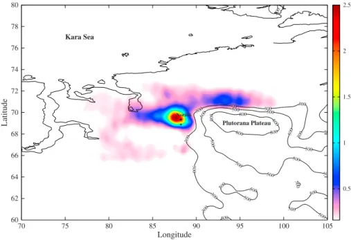
Longitude Latitude 300 300 300 300 300 300 300 300 300 30 300 3 3 500 500 500 500 500 500 500 500 500 500 500 500 50 500 500 500 500 500 800 800 800 800 800 Norilsk Plutorana Plateau Kara Sea 70 75 80 85 90 95 100 105 60 62 64 66 68 70 72 74 76 78 80 0.5 1 1.5 2 2.5
Figure 2. Distribution of the average retrieved 0–2 km SO2columns over the Norilsk region for February 2009, expressed in Dobson units. The average has been performed on a0.25◦× 0.25◦grid and then interpolated. The contour on the plot shows the terrain height in meters.
To calculate the𝐒𝜖for each period, about 20,000 IASI spectra from 2010 and 2011 have been used. Only those with less than 25% of cloud coverage (information taken from European Organisation for the Exploita-tion of Meteorological Satellites (EUMETSAT) L2 products, [August et al., 2012]) and with no detectable SO2 were selected. For this, observed spectra relatively far from the source region were used (60–62◦N/75–100◦E and 74–75◦N/75–100◦E). This area usually does not exhibit observable quantities of SO2(see Figure 2). In
addition, to account for possible residual transported SO2plumes from volcanic origin, data were filtered
using a brightness temperature difference sensitive to SO2[Clarisse et al., 2008]. The corresponding
simu-lated spectra were calcusimu-lated for the spectral range 1330–1390 cm−1with the Atmosphit software [Coheur
et al., 2005]. Temperature and humidity profiles used in the simulations were taken from EUMETSAT L2 products [Schlüssel et al., 2005; August et al., 2012]. This was also the case for the surface temperature, if available. When surface temperature was not included in the L2, it was evaluated by averaging the bright-ness temperature of six window channels (857.50, 866.25, 868.50, 879.00, 892.75, and 1231.75 cm−1). Vertical
profiles of other atmospheric constituents have been taken from the standard subarctic models (winter and summer) [Anderson et al., 1986] defining average volume mixing ratios (vmr) for methane (CH4) and nitrous oxide (N2O), which mainly absorbe the radiation in the covered spectral range along with water. The CH4 model profile was scaled by a factor of 1.06, to bring surface vmr to 1800 ppm, in agreement with surface measurements (see, e.g., http://www.esrl.noaa.gov/gmd/aggi/).
3.3. Retrieval Parameters
Just as for forward simulations, retrievals have been performed with the Atmosphit software in the spec-tral range 1330–1390 cm−1and on spectra with less than 25% of cloud coverage. The chosen reduced state
vector𝐱 contains two SO2columns, the first one extending from 0 to 2 km and the second one from 2 to 5 km. We expect indeed negligible amounts of SO2above 5 km, given the short lifetime of this gas in gen-eral. Furthermore, more specifically for the winter cases analyzed here, the presence of strong temperature inversions confines the pollution at near-surface level. The standard subarctic SO2profile [Anderson et al.,
1986] has been used for the a priori profile, but a large variability of 150% has been considered for the diag-onal elements of the a priori covariance matrix𝐒𝐚to allow retrievals of high concentrations which occur frequently [AMAP, 2006]. The off-diagonal elements have been calculated using an exponential decay with 7 km correlation length. The fixed parameters have been chosen the same as for the forward simulations. The complete retrieval scheme has been applied on IASI spectra recorded for 4 years, between the 1 January 2008 and the 31 December 2011 in a large area around Norilsk (61–75◦N/75–96◦E and 67–75◦N/96–100◦E).
Figure 3. (first panel) Daily average retrieved SO2columns (0–2 km), expressed in DU; (second panel) daily maximum SO2columns (0–2 km, DU); (third panel) daily average thermal contrasts, calculated as the difference between the sur-face temperature and the temperature at 350 m above the ground; (fourth panel) daily average water vapor amount at 350 m, expressed in g/kg. All averages have been calculated for data in a circle of 50 km radius centered on Norilsk, for the period 1 January 2008 to 31 December 2011. Data from morning and evening IASI overpasses have been simultane-ously averaged for SO2columns and the distinction is made for the thermal contrast and water vapor. Note that some measurements are missing for some days. They correspond to gaps in the data or cloudy scenes and have therefore been filtered.
4. Results and Discussion
4.1. Spatial Distribution
Figure 2 presents the spatial distribution of the average retrieved 0–2 km column of SO2for February 2009.
The highest mean retrieved columns are above 2 Dobson units (1 DU = 2.69 × 10¹⁶molecules/cm2) and
situ-ated above the city. The plume spreads away from the source, as seen by a gradual decrease of the retrieved concentrations. Averaged over 1 month, it seems that the pollution plume follows two distinctive trans-port pathways, one eastward and the other westward, surrounding the mountains. The entire SO2plume
observed by IASI covers a large region of about 165,000 km2around Norilsk, suggesting a significant
influ-ence on its surrounding environment, as discussed in Vlasova et al. [1991], Tutubalina and Rees [2001], and Zubareva et al. [2003]. It is worth noting that we can distinctly observe the plume following the Plutorana Plateau (the concentrations above 300 m never being higher than 0.5 DU). This clearly demonstrates that the detected SO2is located close to the surface, where the temperature inversions develop. Actually, the mean altitude of these inversion layers, calculated over the whole retrieved area for February 2009, and based on the temperature profiles provided by the EUMETSAT L2 products, is 410 m above the ground. Most of the SO2pollution is thus probably being transported below this altitude. Similar SO2distributions can be
drawn for other winter months. However, during summer and midseason, higher humidity and lower ther-mal contrasts hamper measurement of near-surface SO2. The detection is only possible for some days, with
particular favorable conditions (see also Figure 3). In contrast, during the winter and as shown in Figure 3 (discussed hereafter), thermal contrasts and humidity are quite homogenously favorable in the area. We can thus reasonably assume that, during winter months, our mean retrieved SO2columns are representative of
near-surface SO2amounts.
4.2. Time Series
Time series of the surface retrieved SO2column are presented in Figure 3 (first panel) for the period 1
of 50 km radius centered on Norilsk. However, in summer and midseason notably, average columns can be strongly underestimated due to changes in PBL sensitivity and thus do not correspond to the real pollution above the area. Moreover, the average is made over a quite large area around Norilsk and is thus not very representative of the high concentrations of SO2just above the city. Therefore, daily maximum SO2columns are also presented in Figure 3 (second panel). The third and fourth panels of Figure 3 show, respectively, the mean thermal contrasts, calculated as the difference between the temperature of the surface and of the air at 350 m altitude (both temperature are from the operational L2) above the ground, and mean humid-ity (at 350 m), calculated over the same area as the SO2columns and for the same period. The altitude of
350 m above the ground was chosen to be equal to the average altitude of the temperature inversion (cal-culated here for the area of interest and only for winter months), below which most of the gas is probably located and which is also the altitude where the peak sensitivity is expected. In Figure 3, the SO2
measure-ments from morning and evening overpasses have been averaged together. In wintertime, solar radiation at the latitude of Norilsk is low (or even vanishing during the polar night), and surface, atmospheric tempera-tures, and humidity are similar during day and night (see green and red curves in Figure 3, third and fourth panels). Therefore, the IASI sensitivity to boundary layer SO2is identical in the two cases. However, in
sum-mer, the diurnal variability of temperatures and humidity is high: differences of more than 10 K of thermal contrast and of more than 5 g/kg of water vapor can occur between day and night (Figure 3). This variability is such that the sensitivity can be very different between the two IASI overpasses, leading to differences in SO2measurements. For the same reasons as those explained above, calculating an average concentration
for the midseason and summer periods, which are already difficult to retrieve due to the weaker sensitivity, produces large underestimation. This is well seen in Figure 3, with the average concentrations from May to October being below 5 DU and essentially close to 0, while daily maximum values can be significantly larger, typically up to 10 DU and in few cases even 50 DU. It can be seen from Figure 3 that retrievals during the summer and the midseason have been possible for days (morning and/or evening) combining exceptionally low humidity and high thermal contrasts (in absolute value). Both conditions coexist, for example, in April 2008, August 2008, September 2008, July 2009, April 2010, May 2010, July 2010, and May 2011. Note that in August 2008, most of the detected SO2was probably emitted by the Kasatochi eruption and transported
over the Norilsk’s region [Karagulian et al., 2010]. Midseason and summer retrieved SO2columns are hence
only qualitatively discussed in the following.
Although the number of successful retrievals is much larger in winter owing to the more favorable condi-tions for detecting boundary layer pollution, we observe also a large variability of SO2columns. Daily means
range from 0.04 DU (the a priori column) to about 20 DU in February 2011. Most columns, however, vary between 1 and 5 DU. Maximum columns reach 50 DU on several days. It clearly appears that most days for which SO2concentrations are close to the a priori correspond to situations where IASI measurements are
not sensitive to the boundary layer, when thermal contrasts are close to zero. Humidity stays low for the entire winter and therefore does not contribute to the loss of sensitivity. This kind of unfavorable winter episodes occurs for instance in January 2008, end of March 2008, November 2008, January 2009, beginning of November 2009, November 2010, end of January 2011, end of March 2011, and December 2011. There are several previous reports of SO2measurements in Norilsk, which were made either by surface instruments [Fukasawa et al., 2000], airplanes [Walter et al., 2012], or satellites using reflected solar radia-tion in the UV-visible [Walter et al., 2012; Fioletov et al., 2013]. Table 1 summarizes the different available SO2measurements and compares them to this work. Although the direct comparison is difficult because
they are not colocated in time and space and refer to different quantities (surface concentrations or vmr, integrated columns), we find that our values are in good agreement with these, especially with the ver-tical columns reported by Walter et al. [2012], which were retrieved from UV satellite measurements. Our retrieved SO2concentrations are in contrast smaller than those measured by Fukasawa et al. [2000] and
those reported by the AMAP [2006] during the 1990s. This is likely due to the fact that these concentrations were measured at the surface while our averaged concentrations were calculated over a 0–2 km layer. As we have demonstrated above, the main SO2column is likely to be confined to a smaller layer, and therefore, our
reported SO2concentrations are biased low. This difference could also be explained by potential reductions
of Norilsk’s SO2emissions. For instance, Walter et al. [2012], referring to a report of the Norwegian Council
on Ethics [Council on Ethics for the Government Pension Fund Global, 2009], mention that the company MMC Norilsk Nickel, which is the head of Norilsk smelting facilities, planned to reduce its SO2emissions by 70%
Table 1. Comparison Between Different Available SO2Measurements Made in the Norilsk Regiona
SO2Measurements Period Comments
This work Daily winter averages of the 0–2 km 2008–2011 Satellite (IASI) column, of the 50 km radius area around
Norilsk, fluctuate:
10–30 ppb, maximum of 105 ppb 20–75μg/m3, maximum of 280μg/m3
0.4–1.5 × 10¹⁷molecules/cm2, maximum of5 × 1017molecules/cm2
Fukasawa et al. [2000] Half month averages fluctuating April–December 1995 Surface
between 30 and 60 ppb Maximum averages of 140 ppb
Khokhar et al. [2004, 2005] Slant column density of about2 × 1016 Average over Satellite
molecules/cm2 1996–2002 (GOME)
AMAP [2006] Annual averages fluctuate between 70 1990–2003
and 210μg/m3
Walter et al. [2012] Slant column density of about8 × 1017 22 October 2010 Aircraft
molecules/cm2at about 5 km of Norilsk
Vertical column density in the range of Satellite (OMI)
0.5–2 × 10¹⁷molecules/cm2
Fioletov et al. [2013] Average values of5.4–6.7 × 10¹⁶ 2005–2010 Satellite (OMI,
molecules/cm2 (depends on SCIAMACHY,
instrument) and GOME-2)
aThe slant column density corresponds to the SO
2concentration integrated along the light path. SO2volume mixing ratios (vmrs) and concentrations given
for this work have been calculated from the IASI retrieved 0–2 km columns. They, respectively, represent the mean vmr and the mean concentration of SO2in the 0–2 km atmospheric layer.
been observed.” Although the comparison provided here may be evidence of the impact of emission regu-lations, a definitive conclusion would require more investigation and validation of the IASI measurements.
4.3. Winter Emissions
From the IASI SO2measurements, we have estimated the winter emissions of the Norilsk sources. We have
first calculated daily SO2total masses M according to the relation:
M(SO2) = MSO2CSO2S Na
(2) where MSO2is the molar mass of SO2(64.0638 g/mol), CSO2is the mean SO2total column (here calculated
as the sum of the 0–2 km and 2–5 km retrieved columns) in molecules/cm2for the chosen box of surface
area S, and Nais the Avogadro number. SO2masses have been calculated for each 0.25◦ × 0.25◦box of a grid covering the entire retrieved area (60–75◦N/75–100◦E), and then summed to obtain the SO2total mass for the region. To avoid underestimation of the total masses because of lack of sensitivity on some days in winter (obvious in Figure 3 from the low column averages), only measurements with thermal contrast higher or equal than 10 K in absolute value were taken into account. Averaged SO2columns were then interpolated
from 1 month of data, for each box of the grid. In this way, a mean daily total mass for the entire region is estimated for each month.
The emissions for the winter months have then been calculated using a simple box model and first-order loss terms [Jacob, 1999]:
Ei+1(SO2) =
Mi+1(SO2) − Mi(SO2)e−t∕𝜏eff
𝜏eff(1 − e−t∕𝜏eff)
(3)
Ei(SO2) and Mi(SO2) are, respectively, the emission and total mass of SO2for the day i,𝜏effis the effective
lifetime of SO2, and t is time between two observations (here 1 day). Because we have estimated a mean
daily total mass for each month, the previous equation simplifies in E = M∕𝜏effand leads to constant daily
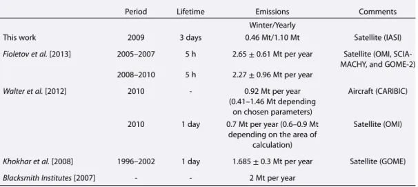
Table 2. Norilsk’s Winter Emissions Derived From IASI SO2Measurementsa
Period Lifetime Emissions Comments Winter/Yearly
This work 2009 3 days 0.46 Mt/1.10 Mt Satellite (IASI)
Fioletov et al. [2013] 2005–2007 5 h 2.65±0.61 Mt per year Satellite (OMI, SCIA-MACHY, and GOME-2) 2008–2010 5 h 2.27±0.96 Mt per year
Walter et al. [2012] 2010 - 0.92 Mt per year Aircraft (CARIBIC)
(0.41–1.46 Mt depending on chosen parameters)
2010 1 day 0.7 Mt per year (0.6–0.9 Mt Satellite (OMI) depending on the area of
calculation)
Khokhar et al. [2008] 1996–2002 1 day 1.685±0.3 Mt per year Satellite (GOME)
Blacksmith Institutes [2007] - - 2 Mt per year
aEmissions obtained in other studies are also presented. For all, the period and the chosen lifetime (if required in
the study) are given. Winter includes five cold months: January, February, March, November, and December.
which the IASI sensitivity to boundary layer is the highest. Only emissions calculated for 2009 are discussed hereafter, because this year presents the largest and the most constant amount of available data.
The choice of the lifetime is crucial in estimating the emission. Lee et al. [2011] have calculated the seasonal zonal mean lifetime of SO2in the boundary layer using the GEOS-Chem model. They show that it is very variable with season and latitude, mainly because of changes in dry deposition velocities and in supply of oxidants. For high latitudes, a lifetime of about 1 day in summer to more than 3 days in winter was obtained. In wintertime and particularly during the polar night, SO2lifetime is longer than for the summer, because of
smaller concentrations of oxidants and reduced velocities of dry deposition due to snow coverage [Chin and Jacob, 1996; Wesely, 2007]. Here we used a SO2lifetime of 3 days representative of winter conditions.
Table 2 compares SO2emissions derived in this work and in other studies. Emissions for 2009 from IASI add
up to 0.46 Mt in the winter and 1.10 Mt for the whole year. Yearly totals were calculated from the winter months, assuming constant emissions. This is a reasonable assumption as smelting facilities usually run con-tinuously (24 h per day, 7 days per week). This value is in good agreement with Khokhar et al. [2008] and Walter et al. [2012]. Total emissions reported in Blacksmith Institutes [2007] and Fioletov et al. [2013] are about a factor of 2 larger. However, the latter study uses a rather short SO2lifetime of 5 h. It is also possible that the winter SO2lifetime is larger than the 3 days which we have used. It is clear that SO2lifetime has to be better constrained to make more accurate estimation of emissions from satellite measurements.
4.4. Estimation of the Retrieval Error
In this section, we estimate the error on the IASI retrieved SO2columns independently of the diagnostics of the Optimal Estimation method, which are highly dependent on the a priori constraints. As there are also no suitable independent measurements available for validation, an alternative approach has been developed based on retrievals of a set of synthetic IASI spectra with known SO2columns. This allows a rigorous
esti-mate of the errors characterized by the global error spectral covariance matrix𝐒𝜖, which includes the IASI noise, uncertainties in relevant meteorological parameters, in the spectroscopy of interfering trace gases and radiative transfer.
The synthetic IASI spectra have been generated with 340 randomly chosen SO2columns and
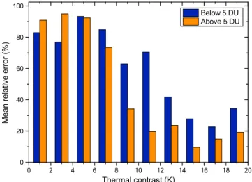
represen-tative surface temperatures, temperature, and humidity profiles for the winter months in Norilsk. Then a synthetic noise was added, generated from the multivariate normal distribution corresponding to the𝐒𝜖 matrix. From these spectra, SO2was retrieved in exactly the same way as for the observed IASI spectra. The relative difference between the input and the retrieved columns then gives the error term described above. A histogram of the errors as a function of thermal contrast (in absolute value) and the 0–2 km SO2column
is shown in Figure 4. A clear dependence of the errors on the thermal contrast is observed: for thermal con-trasts above 12 K the errors range from 10% to 40%, between 20% and 85% for thermal concon-trasts between 6 and 12 K, and finally above 80% for thermal contrasts below 6 K. When thermal contrast is small, there is little
Figure 4. Histogram of the relative error on the 0–2 km SO2column as a function of thermal contrast (absolute value). The relative error is calculated according to the relation:[(SO2column)true−(SO2column)retrieved]∕(SO2column)true×100%. Bars represent the mean error calculated for fields of 2 K range of thermal contrast. The blue bars are the mean error for columns smaller than 5 DU and the orange are the mean error for columns larger than 5 DU.
sensitivity to PBL SO2and the retrieval depends only on the choice of the a priori. As it increases,
sensi-tivity to the PBL increases and the retrieved values match closer the real ones. The magnitude of the SO2
columns also has an effect on the sensitivity, as larger columns yield larger spectral signatures and hence larger signal to noise ratios. This can be seen in Figure 4, where the distinction was made for columns below (blue columns) and above (orange columns) 5 DU. However, even for very large thermal contrasts and large columns, there is a low bias of about 15% for the larger SO2columns. This difference could be due to an
imperfect training set used in the generation of the𝐒𝜖matrix (e.g., with residual SO2signatures present).
Another possibility is that the presence of spectral interferences, irrecoverably masks part of the SO2
sig-nature, and hence leads to an underestimation of the SO2column. Overall, relative errors are on average
below 30% for thermal contrasts exceeding 12 K, a result which shows that thermal infrared sounders can in favorable conditions probe the PBL with high accuracy. We also investigated the influence of water vapor on the retrieval error as larger H2O columns are expected to adversely affect the retrieval. However, wintertime conditions in Norilsk are dry (less than 1 g/kg of H2O at 350 m) and constant, so that no dependence was
found here.
One category of errors not accounted for here, relates to the strength of the SO2spectral signature (for a given column). These include errors in the spectroscopic parameters, uncertainties on the SO2profile, and the impact of the thermal contrast on the SO2lines in the forward model. Independent validation would be
required to properly estimate such errors.
5. Conclusions
We have obtained the first IASI distributions of SO2at near-surface level, using 4 years of measurements in a large area (61–75◦N/75–96◦E and 67–75◦N/96–100◦E) around the polluted city of Norilsk in the Arctic circle. Retrievals were performed using a methodology based on the Optimal Estimation and where a full𝐒𝜖 spec-tral variance-covariance matrix was used to account for interfering atmospheric parameters. Time series of the retrieved SO20–2 km partial column have been investigated and revealed a strong dependence of the
sensitivity of IASI to the polluted surface layer on thermal contrast and humidity. In wintertime, when there is a combination of dry conditions and frequent temperature inversions, large SO2columns (around 5 DU
on average but up to 50 DU occasionally) have been successfully retrieved for many days. In favorable con-ditions, retrieval errors can be as low as 10%, but depending on thermal contrast and SO2column, can reach up to 95%. In the summer months, retrievals are harder due to lower values of thermal contrast coupled with larger atmospheric humidity, which renders the atmosphere opaque in the lowest layers. For some days in summer, however, successful retrievals have been obtained, giving daily maximum SO2columns typically
as IASI largely complement observations of UV instruments at high-latitude regions, as the sounding of the latter is impossible during this period as solar radiation is unavailable.
The yearly emissions of SO2for the Norilsk area have been estimated from the retrieved columns in the
winter months, using a simple box model and first-order loss terms, and assuming constant emissions. For a lifetime of 3 days, we obtained a yearly emission of 1.10 Mt. This value is in reasonable agreement with those obtained by other satellite sounders operating in the UV-visible and other type of remote-sensing instruments. Validation of the SO2measurements of this work and a better evaluation of the lifetime of SO2,
present at high latitudes and in a polluted plume, are required to allow drawing conclusions.
More generally, the results presented in this work open unexpected perspectives for the monitoring of air quality with TIR satellite sounders, by extending it to other pollutants and other regions with favorable ther-mal contrast conditions. Recently, a severe pollution episode, which occurred in the North China Plain in January 2013, has been analyzed by Boynard et al. [2014], who provided simultaneous observations of SO2
and other pollutants by exploiting the enhanced sensitivity of IASI in cases of temperature inversion.
References
Allen-Gil, S. M., J. Ford, B. K. Lasorsa, M. Monetti, T. Vlasova, and D. H. Landers (2003), Heavy metal contamination in the Taimyr Peninsula, Siberian Arctic, Sci. Total Environ., 301, 119–138, doi:10.1016/S0048-9697(02)00295-4.
Arctic Monitoring and Assessment Programme (AMAP) (1998), Acidifying Pollutants, Arctic Haze, and Acidification in the Arctic, 621–659, Arctic Monitoring and Assessment Programme (AMAP), Oslo.
Arctic Monitoring and Assessment Programme (AMAP) (2006), AMAP Assessment 2006: Acidifying Pollutants, Arctic Haze, and Acidification
in the Arctic, Arctic Monitoring and Assessment Programme (AMAP), Oslo, Norway.
Anderson, G., S. Clough, F. Kneizys, J. Chetwynd, and E. P. Shettle (1986), AFGL Atmospheric Constituent Profiles (0-120km),
Environmental Research Papers No. 954, ADA175173, AFGL-TR 86-0110, U.S. Air Force Geophysics Laboratory. Optical Physics Division.
August, T., D. Klaes, P. Schlüssel, T. Hultberg, M. Crapeau, A. Arriaga, A. O’Carroll, D. Coppens, R. Munro, and X. Calbet (2012), IASI on Metop-A: Operational Level 2 retrievals after five years in orbit, J. Quant. Spectrosc. Radiat. Transfer, 113, 1340–1371, doi:10.1016/j.jqsrt.2012.02.028.
Blacksmith Institutes (2007), The World’s Worst Polluted Places - The Top Ten of the Dirty Thirty, Blacksmith Institutes, New York. Blais, J. M., K. E. Duff, T. E. Laing, and J. P. Smol (1999), Regional contamination in lakes from the Noril’sk region in Siberia, Russia, Water
Air Soil Pollut., 110, 389–404, doi:10.1023/A:1005059325100.
Boyd, R., S.-J. Barnes, P. De Caritat, V. A. Chekushin, V. A. Melezhik, C. Reimann, and M. L. Zientek (2009), Emissions from the copper–nickel industry on the Kola Peninsula and at Norilsk, Russia, Atmos. Environ., 43, 1474–1480, doi:10.1016/j.atmosenv.2008.12.003.
Boynard, A., et al. (2014), First space measurements of simultaneous pollutants in the boundary layer from IASI: A case study in the North China Plain, Geophys. Res. Lett., 41, 1–6, doi:10.1002/2013GL058333.
Carboni, E., R. Grainger, J. Walker, A. Dudhia, and R. Siddans (2012), A new scheme for sulphur dioxide retrieval from IASI measurements: Application to the Eyjafjallajökull eruption of April and May 2010, Atmos. Chem. Phys., 12, 11,417–11,434, doi:10.5194/acp-12-11417-2012.
Carn, S. A., A. J. Krueger, N. A. Krotkov, and M. A. Gray (2004), Fire at Iraqi sulfur plant emits SO2clouds detected by Earth Probe TOMS,
Geophys. Res. Lett., 31, L19105, doi:10.1029/2004GL020719.
Carn, S. A., A. J. Krueger, N. A. Krotkov, K. Yang, and P. F. Levelt (2007), Sulfur dioxide emissions from Peruvian copper smelters detected by the Ozone Monitoring Instrument, Geophys. Res. Lett., 34, L09801, doi:10.1029/2006GL029020.
Chin, M., and D. J. Jacob (1996), Anthropogenic and natural contributions to tropospheric sulfate: A global model analysis, J. Geophys.
Res., 101, 18,691–18,699, doi:10.1029/96JD01222.
Clarisse, L., P.-F. Coheur, A. J. Prata, D. Hurtmans, A. Razavi, T. Phulpin, J. Hadji-Lazaro, and C. Clerbaux (2008), Tracking and quantifying volcanic SO2with IASI, the September 2007 eruption at Jebel at Tair, Atmos. Chem. Phys., 8, 7723–7734, doi:10.5194/acp-8-7723-2008. Clarisse, L., M. W. Shephard, F. Dentener, D. Hurtmans, K. Cady-Pereira, F. Karagulian, M. Van Damme, C. Clerbaux, and P.-F. Coheur (2010),
Satellite monitoring of ammonia: A case study of the San Joaquin Valley, J. Geophys. Res., 115, D13302, doi:10.1029/2009JD013291. Clarisse, L., Y. R’Honi, P.-F. Coheur, D. Hurtmans, and C. Clerbaux (2011a), Thermal infrared nadir observations of 24 atmospheric gases,
Geophys. Res. Lett., 38, L10802, doi:10.1029/2011GL047271.
Clarisse, L., M. Fromm, Y. Ngadi, L. Emmons, C. Clerbaux, D. Hurtmans, and P.-F. Coheur (2011b), Intercontinental transport of anthropogenic sulfur dioxide and other pollutants: An infrared remote sensing case study, Geophys. Res. Lett., 38, L19806, doi:10.1029/2011GL048976.
Clarisse, L., D. Hurtmans, C. Clerbaux, J. Hadji-Lazaro, Y. Ngadi, and P.-F. Coheur (2012), Retrieval of sulphur dioxide from the infrared atmospheric sounding interferometer (IASI), Atmos. Meas. Tech., 5, 581–594, doi:10.5194/amt-5-581-2012.
Clerbaux, C., et al. (2009), Monitoring of atmospheric composition using the thermal infrared IASI/MetOp sounder, Atmos. Chem. Phys., 9, 6041–6054, doi:10.5194/acp-9-6041-2009.
Coheur, P.-F., B. Barret, S. Turquety, D. Hurtmans, J. Hadji-Lazaro, and C. Clerbaux (2005), Retrieval and characterization of ozone vertical profiles from a thermal infrared nadir sounder, J. Geophys. Res., 110, D24303, doi:10.1029/2005JD005845.
Council on Ethics for the Government Pension Fund Global (2009), Annual report 2009.
Deeter, M. N., D. P. Edwards, J. C. Gille, and J. R. Drummond (2007), Sensitivity of MOPITT observations to carbon monoxide in the lower troposphere, J. Geophys. Res., 112, D24306, doi:10.1029/2007JD008929.
Fioletov, V. E., C. A. McLinden, N. Krotkov, M. D. Moran, and K. Yang (2011), Estimation of SO2emissions using OMI retrievals, Geophys.
Res. Lett., 38, L21811, doi:10.1029/2011GL049402.
Fioletov, V. E., et al. (2013), Application of OMI, SCIAMACHY, and GOME-2 satellite SO2retrievals for detection of large emission sources,
J. Geophys. Res. Atmos., 118, 11,399–11,418, doi:10.1002/jgrd.50826.
Fukasawa, T., S. Ohta, K. Enomoto, N. Murao, S. Yamagata, T. Shimizu, V. N. Makarov, and I. Rastegaev (2000), Measurement of air pollution in Norilsk, Polar Meteorol. Glaciol., 14, 92–102.
Acknowledgments
IASI has been developed and built under the responsibility of the Centre National d’Etudes Spatiales (CNES, France). It is flown on board the MetOp satellites as part of the EUMETSAT Polar System. The IASI L1 data are received through the EUMETCast near real-time data dis-tribution service. The research in Belgium was funded by the F.R.S-FNRS, the Belgian State Federal Office for Scientific, Technical, and Cultural Affairs, and the European Space Agency (ESA-Prodex arrangements). Financial support by the “Actions de Recherche Concertées” (Communauté Française de Belgique) is also acknowl-edged. S. Bauduin and P.-F. Coheur are, respectively, Research Fellow and Senior Research Associate with F.R.S.-FNRS. C. Clerbaux is grateful to CNES for scientific collaboration and financial support.
Haywood, J. M., et al. (2010), Observations of the eruption of the Sarychev volcano and simulations using the HadGEM2 climate model,
J. Geophys. Res., 115, D21212, doi:10.1029/2010JD014447.
Hilton, F., et al. (2012), Hyperspectral Earth observation from IASI - Five years of accomplishments, Bull. Am. Meteorol. Soc., 93, 347–370, doi:10.1175/BAMS-D-11-00027.1.
Hirdman, D., H. Sodemann, S. Eckhardt, J. F. Burkhart, A. Jefferson, T. Mefford, P. K. Quinn, S. Sharma, J. Ström, and A. Stohl (2010), Source identification of short-lived air pollutants in the Arctic using statistical analysis of measurement data and particle dispersion model output, Atmos. Chem. Phys., 10, 669–693, doi:10.5194/acp-10-669-2010.
Jacob, D. J. (1999), Introduction to Atmospheric Chemistry, Princeton Univ. Press, Princeton, N. J.
Karagulian, F., L. Clarisse, C. Clerbaux, A. J. Prata, D. Hurtmans, and P.-F. Coheur (2010), Detection of volcanic SO2, ash, and H2SO4using the Infrared Atmospheric Sounding Interferometer (IASI), J. Geophys. Res., 115, D00L02, doi:10.1029/2009JD012786.
Khokhar, M., U. Platt, and T. Wagner (2008), Temporal trends of anthropogenic SO2emitted by non-ferrous metal smelters in Peru and Russia estimated from Satellite observations, Atmos. Chem. Phys. Discuss., 8, 17,393–17,422, doi:10.5194/acpd-8-17393-2008. Khokhar, M. F., C. Frankenberg, J. Hollwedel, S. Beirle, S. Kühl, M. Grzegorski, W. Wilms-Grabe, U. Platt, and T. Wagner (2004), Satellite
remote sensing of atmospheric SO2: Volcanic eruptions and anthropogenic emissions, in Proc. of the 2004 Envisat & ERS Symposium,
Salzburg, Austria 6-10 September 2004 (ESA SP-572, April 2005), edited by H. Lacoste and L. Ouwehand, pp. 1–8, ESA Publication
Division, ESTEC, Noordwijk, Netherlands.
Khokhar, M. F., C. Frankenberg, M. Van Roozendael, S. Beirle, S. Kühl, A. Richter, U. Platt, and T. Wagner (2005), Satellite obser-vations of atmospheric SO2from volcanic eruptions during the time-period of 1996–2002, Adv. Space Res., 36, 879–887, doi:10.1016/j.asr.2005.04.114.
Krotkov, N. A., et al. (2008), Validation of SO2retrievals from the Ozone Monitoring Instrument over NE China, J. Geophys. Res., 113, D16S40, doi:10.1029/2007JD008818.
Laj, P., et al. (2009), Measuring atmospheric composition change, Atmos. Environ., 43, 5351–5414, doi:10.1016/j.atmosenv.2009.08.020. Law, K. S., and A. Stohl (2007), Arctic air pollution: Origins and impacts, Science, 315, 1537–1540, doi:10.1126/science.1137695. Lee, C., R. V. Martin, A. Van Donkelaar, H. Lee, R. R. Dickerson, J. C. Hains, N. Krotkov, A. Richter, K. Vinnikov, and J. J. Schwab (2011), SO2
emissions and lifetimes: Estimates from inverse modeling using in situ and global, space-based (SCIAMACHY and OMI) observations,
J. Geophys. Res., 116, D06304, doi:10.1029/2010JD014758.
Li, C., Q. Zhang, N. A. Krotkov, D. G. Streets, K. He, S.-C. Tsay, and J. F. Gleason (2010), Recent large reduction in sulfur dioxide emissions from Chinese power plants observed by the Ozone Monitoring Instrument, Geophys. Res. Lett., 37, L08807, doi:10.1029/2010GL042594. Martin, R. V. (2008), Satellite remote sensing of surface air quality, Atmos. Environ., 42, 7823–7843, doi:10.1016/j.atmosenv.2008.07.018. McLinden, C. A., V. Fioletov, K. F. Boersma, N. Krotkov, C. E. Sioris, J. P. Veefkind, and K. Yang (2012), Air quality over the Canadian oil
sands: A first assessment using satellite observations, Geophys. Res. Lett., 39, L04804, doi:10.1029/2011GL050273. Rodgers, C. D. (2000), Inverse Methods for Atmospheric Sounding: Theory and Practice, World Sci., Singapore.
Rothman, L., et al. (2009), The HITRAN 2008 molecular spectroscopic database, J. Quant. Spectrosc. Radiat. Transfer, 110, 533–572, doi:10.1016/j.jqsrt.2009.02.013.
Schlüssel, P., T. H. Hultberg, P. L. Phillips, T. August, and X. Calbet (2005), The operational IASI Level 2 processor, Adv. Space Res., 36, 982–988, doi:10.1016/j.asr.2005.03.008.
Tutubalina, O., and W. Rees (2001), Vegetation degradation in a permafrost region as seen from space: Norilsk (1961–1999), Cold Reg. Sci.
Technol., 32, 191–203, doi:10.1016/S0165-232X(01)00049-0.
Van Damme, M., L. Clarisse, C. L. Heald, D. Hurtmans, Y. Ngadi, C. Clerbaux, A. J. Dolman, J. W. Erisman, and P.-F. Coheur (2013), Global dis-tributions and trends of atmospheric ammonia (NH3) from IASI satellite observations, Atmos. Chem. Phys. Discuss., 13, 24,301–24,342, doi:10.5194/acpd-13-24301-2013.
Vlasova, T. M., B. I. Kovalev, and Philipchuk (1991), Effects of point source atmospheric pollution on boreal forest vegetation of Northern Siberia, in Proceedings of the International Conference on the Role of the Polar Regions in Global Change, vol. 2, edited by G. Weller, C. L. Wilson, and B. A. B. Sever, pp. 423–428, Univ. of Alaska, Fairbanks.
Walter, D., K.-P. Heue, A. Rauthe-Schöch, C. A. M. Brenninkmeijer, L. N. Lamsal, N. A. Krotkov, and U. Platt (2012), Flux calculation using CARIBIC DOAS aircraft measurements: SO2emission of Norilsk, J. Geophys. Res., 117, D11305, doi:10.1029/2011JD017335. Wesely, M. L. (2007), Parameterization of surface resistances to gaseous dry deposition in regional-scale numerical models, Atmos.
Environ., 41, S52–S63, doi:10.1016/j.atmosenv.2007.10.058.
Zubareva, O. N., L. N. Skripal’shchikova, N. V. Greshilova, and V. I. Kharuk (2003), Zoning of landscapes exposed to technogenic emissions from the Norilsk mining and smelting works, Russ. J. Ecol., 34(6), 375–380, doi:10.1023/A:1027356316112.