HAL Id: hal-00618812
https://hal.archives-ouvertes.fr/hal-00618812
Submitted on 19 Dec 2015
HAL is a multi-disciplinary open access
archive for the deposit and dissemination of
sci-entific research documents, whether they are
pub-lished or not. The documents may come from
teaching and research institutions in France or
abroad, or from public or private research centers.
L’archive ouverte pluridisciplinaire HAL, est
destinée au dépôt et à la diffusion de documents
scientifiques de niveau recherche, publiés ou non,
émanant des établissements d’enseignement et de
recherche français ou étrangers, des laboratoires
publics ou privés.
Arctic pollution using aircraft, ground-based, satellite
observations and MOZART-4 model: source attribution
and partitioning
C. Wespes, L. Emmons, D. P. Edwards, J. Hannigan, Daniel Hurtmans, M.
Saunois, Pierre-François Coheur, Cathy Clerbaux, M. T. Coffey, R. Batchelor,
et al.
To cite this version:
C. Wespes, L. Emmons, D. P. Edwards, J. Hannigan, Daniel Hurtmans, et al.. Analysis of ozone and
nitric acid in spring and summer Arctic pollution using aircraft, ground-based, satellite observations
and MOZART-4 model: source attribution and partitioning. Atmospheric Chemistry and Physics,
European Geosciences Union, 2012, 12 (1), pp.237-259. �10.5194/acp-12-237-2012�. �hal-00618812�
Atmos. Chem. Phys., 12, 237–259, 2012 www.atmos-chem-phys.net/12/237/2012/ doi:10.5194/acp-12-237-2012
© Author(s) 2012. CC Attribution 3.0 License.
Atmospheric
Chemistry
and Physics
Analysis of ozone and nitric acid in spring and summer Arctic
pollution using aircraft, ground-based, satellite observations and
MOZART-4 model: source attribution and partitioning
C. Wespes1, L. Emmons1, D. P. Edwards1, J. Hannigan1, D. Hurtmans2, M. Saunois1, P.-F. Coheur2, C. Clerbaux2,3, M. T. Coffey1, R. L. Batchelor1, R. Lindenmaier4, K. Strong4, A. J. Weinheimer1, J. B. Nowak5,6, T. B. Ryerson5, J. D. Crounse7, and P. O. Wennberg7
1National Center for Atmospheric Research, Boulder, CO, USA
2Chimie Quantique et Photophysique, Universit´e Libre de Bruxelles, Brussels, Belgium
3UPMC Univ. Paris 6; Universit´e Versailles St.-Quentin, CNRS/INSU, LATMOS-IPSL, Paris, France 4Department of Physics, University of Toronto, Toronto, ON, Canada
5NOAA, Earth System Research Laboratory, Boulder, CO, USA
6Cooperative Institute for Research in Environmental Sciences (CIRES), University of Colorado, Boulder, CO, USA 7California Institute of Technology, Pasadena, CA, USA
Correspondence to: C. Wespes ([email protected])
Received: 13 July 2011 – Published in Atmos. Chem. Phys. Discuss.: 22 August 2011 Revised: 12 December 2011 – Accepted: 14 December 2011 – Published: 4 January 2012
Abstract. In this paper, we analyze tropospheric O3together
with HNO3during the POLARCAT (Polar Study using
Air-craft, Remote Sensing, Surface Measurements and Models, of Climate, Chemistry, Aerosols, and Transport) program, combining observations and model results. Aircraft obser-vations from the NASA ARCTAS (Arctic Research of the Composition of the Troposphere from Aircraft and Satel-lites) and NOAA ARCPAC (Aerosol, Radiation and Cloud Processes affecting Arctic Climate) campaigns during spring and summer of 2008 are used together with the Model for Ozone and Related Chemical Tracers, version 4 (MOZART-4) to assist in the interpretation of the observations in terms of the source attribution and transport of O3and HNO3into the
Arctic (north of 60◦N). The MOZART-4 simulations repro-duce the aircraft observations generally well (within 15 %), but some discrepancies in the model are identified and dis-cussed. The observed correlation of O3 with HNO3 is
ex-ploited to evaluate the MOZART-4 model performance for different air mass types (fresh plumes, free troposphere and stratospheric-contaminated air masses).
Based on model simulations of O3and HNO3tagged by
source type and region, we find that the anthropogenic pollu-tion from the Northern Hemisphere is the dominant source of O3and HNO3in the Arctic at pressures greater than 400 hPa,
and that the stratospheric influence is the principal
contribu-tion at pressures less 400 hPa. During the summer, intense Russian fire emissions contribute some amount to the tro-pospheric columns of both gases over the American sector of the Arctic. North American fire emissions (California and Canada) also show an important impact on tropospheric ozone in the Arctic boundary layer.
Additional analysis of tropospheric O3 measurements
from ground-based FTIR and from the IASI satellite sounder made at the Eureka (Canada) and Thule (Greenland) po-lar sites during POLARCAT has been performed using the tagged contributions. It demonstrates the capability of these instruments for observing pollution at northern high lati-tudes. Differences between contributions from the sources to the tropospheric columns as measured by FTIR and IASI are discussed in terms of vertical sensitivity associated with these instruments. The first analysis of O3 tropospheric
columns observed by the IASI satellite instrument over the Arctic is also provided. Despite its limited vertical sensi-tivity in the lowermost atmospheric layers, we demonstrate that IASI is capable of detecting low-altitude pollution trans-ported into the Arctic with some limitations.
1 Introduction
As a part of the international POLARCAT (Polar Study using Aircraft, Remote Sensing, Surface Measurements and Mod-els, of Climate, Chemistry, Aerosols, and Transport) pro-gram of field observations of Arctic atmospheric composi-tion during the 2007–2008 Internacomposi-tional Polar Year, the Arc-tic Research of the Composition of the Troposphere from Aircraft and Satellites (ARCTAS) and Aerosol, Radiation, and Cloud Processes affecting Arctic Climate (ARCPAC) missions were conducted during spring and summer 2008 to better understand factors driving change in the atmospheric composition and climate of the Arctic (Jacob et al., 2010; Brock et al., 2011). Cool surface temperature and stable con-ditions characteristic of the Arctic atmosphere facilitate low-altitude isentropic transport into this region, making it a ma-jor receptor for mid-latitude pollution (Klonecki et al., 2003; Stohl, 2006). This process produces the so-called “Arctic Haze”, a recurring phenomenon observed every winter and spring, that results from long-range transport of aerosols and persistent pollutants such as mercury and ozone (O3).
Pre-vious studies based on Arctic measurements from ground stations, aircraft, sondes and satellites, which provide ob-servations of several trace species, show that the Arctic tro-posphere is strongly influenced by emissions from Europe, North America and Asia. They particularly showed that transport from anthropogenic source regions occurs through different processes at different altitudes: near-surface pollu-tion is dominated by Northern European and North American sources, while Asian sources are the dominant contributors at higher altitudes (e.g., Stohl, 2006; Shindell et al., 2008; Fisher et al., 2010; Tilmes et al., 2011). They also highlight the strong impact of boreal forest fires in North America, Asia and Eastern Europe on the Arctic atmospheric pollution (e.g., Generoso et al., 2007; Leung et al., 2007; Turquety et al., 2007; Stohl et al., 2007; Fisher et al., 2010; Tilmes et al., 2011). However, despite the major interest in Arctic pollution for air quality and climate concerns, there remains considerable uncertainty concerning the source-receptor re-lationships between mid-latitude and Arctic atmospheric pol-lution throughout the troposphere (Shindell et al., 2008).
The ARCTAS and ARCPAC aircraft campaigns, which cover periods of several weeks in spring and summer, pro-vide a large and suitable observational dataset for studying the long-range transport of pollution into the Arctic. The spring period offers a good opportunity to observe Asian in-fluence, which is less understood than transport from Eu-rope. This period is also favorable in terms of photochem-istry controlling ozone production (Jacob et al., 2010) and of stratosphere-troposphere exchange affecting tropospheric ozone and nitric acid (HNO3)in the Arctic. A primary goal
of the summer deployment of ARCTAS was to better char-acterize boreal fire emissions, the chemical evolution within the fire plumes, and the regional scale impact of these forest fires. Another research theme of ARCTAS was to better
un-derstand the chemical processes controlling nitrogen oxides (NOx)in the Arctic (Jacob et al., 2010). NOxplays an
es-sential role in the processes that control the ozone abundance in the lower atmosphere. HNO3is one of the principal
reser-voir species for the nitrogen oxides. Ozone and nitric acid can either be produced in mid-latitude source regions or dur-ing transport into the Arctic from the NOxprecursors. Ozone
production is limited by oxidation of NOxto reservoirs, such
as PAN (peroxyacetlynitrate) and HNO3. Correlations
be-tween NOx, NOy (the sum of all reactive nitrogen species)
and O3have frequently been used as a probe of chemistry
and transport in the lower atmosphere (Murphy et al., 1993; Trainer et al., 1993; Ridley, et al., 1994; Singh et al., 1996; Fischer et al., 2000, Zellweger et al., 2003). Strong correla-tions between HNO3 and O3 were established in the lower
stratosphere/upper troposphere and have been used previ-ously to characterize air masses in the Arctic and midlatitude regions (Bregman et al., 1995; Talbot et al., 1997; Schnei-der et al., 1999; Neuman et al., 2001; Popp et al., 2009), to validate satellite HNO3profiles (Irie et al., 2006; Popp et al.,
2009), or to infer the efficiency of ozone production (Cooper et al., 2011). Study of the correlation of HNO3and O3 in
the lower/middle troposphere is less common, despite its im-portance in quantifying the dependence of ozone on nitrogen compounds. The DC-8 aircraft from the spring and summer ARCTAS mission, as well as the concurrent NOAA WP-3D aircraft for the ARCPAC campaign (Brock et al., 2011), pro-vide relevant information for this purpose.
Another central motivation for the ARCTAS campaign was to augment and interpret satellite observations of at-mospheric composition (Jacob et al., 2010). Here, we show that the high spatiotemporal coverage of the Infrared Atmospheric Sounding Interferometer (IASI) instrument, launched onboard the polar orbiting MetOp satellite in Oc-tober 2006, provides an excellent platform for observing the long-range transport of mid-latitude pollution into the Arc-tic. The comparison of satellite retrievals with aircraft data and chemistry transport model simulations provides a use-ful evaluation of the capability of satellites to measure Arctic atmospheric composition.
We present in this paper an analysis of the sources and the transport of Arctic pollution of O3and HNO3during spring
and summer 2008 using a combination of the MOZART-4 chemical transport model, in situ measurements from air-craft (ARCTAS and ARCPAC campaigns) and remote mea-surements from ground-based Fourier Transform InfraRed (FTIR) and IASI spectrometers. First, a brief description of the model and measurements is given, followed by an evalu-ation of the model using observevalu-ations of O3and HNO3
dur-ing the campaigns in Sect. 3. In Sect. 4, the source attribu-tion and their partiattribu-tioning derived from the “tagging method” are presented. In Sect. 5, tropospheric observations of O3
from FTIR instruments, at the Thule (Greenland) and Eu-reka (Canada) polar sites, and from the IASI satellite dur-ing the aircraft campaigns are discussed in comparison with
C. Wespes et al.: Analysis of ozone and nitric acid in spring and summer Arctic 239
MOZART-4 results. We also use IASI observations to fur-ther investigate the capability of the instrument to observe the sources of pollution and the transport into the Arctic. Con-clusions are given in Sect. 6.
2 Model and measurements 2.1 MOZART-4 model description
For this paper, model simulations were performed with the MOZART-4 global 3-D chemical transport model (Emmons et al., 2010a). It was driven by offline meteorological fields from the National Centers for Environmental Predic-tion (NCEP) Global Forecast System (GFS), with a horizon-tal resolution of 1.4◦×1.4◦(approximately 140 km) with 64 levels from the surface up to 2 hPa. MOZART-4 was run with its standard chemical mechanism, including 97 species and approximately 200 reactions (Emmons et al., 2010a). As described in detail in Emmons et al. (2010a), MOZART-4 does not have a complete chemistry in the stratosphere. For specifying long-lived species in the stratosphere (including O3, CO, CH4, HNO3, NOx), it uses zonal mean
climato-logical values above 50 hPa, coming from MOZART-3 sim-ulations (Kinnison et al., 2007), and then it constrains the mixing ratios by relaxation toward the climatology down to the tropopause. MOZART-4 is also not complete for the troposphere since it does not include halogen chemistry. Our model simulations, covering the period April 2008– July 2008, have been initialized by model simulations at 2.8◦×2.8◦starting July 2007 with 42 levels in the vertical. MOZART-4 simulations of O3and related tracers have been
previously compared to numerous in situ observations and used to track the intercontinental transport of pollution (e.g., Emmons et al., 2010b; Pfister et al., 2006, 2008).
The anthropogenic emissions used here are taken from the 2006 inventory of Zhang et al. (2009). This emission inventory is built upon the INTEX-B inventory with addi-tional data from other inventories to obtain global emis-sions (see http://www.cgrer.uiowa.edu/arctas/emission.html for more information). These emissions are constant in time, with no monthly variation. The emissions for VOCs are only available as total VOCs, so speciation to the MOZART-4 VOCs was based on the VOC speciation of the RETRO emissions inventory, as in Lamarque et al. (2010). The fire emissions were calculated using the global Fire INventory from NCAR (FINN) version 1 (Wiedinmyer et al., 2011). Emissions for individual fires, based on daily MODIS fire counts, were calculated and then gridded to the simulation resolution (Wiedinmyer et al., 2006, 2011). Aircraft emis-sions of NO, CO and SO2from general aviation and military
traffic for 1999 are also taken into account (Emmons et al., 2010a). Other natural emissions, for example, NO from soil and lightning are also included in the standard MOZART-4 scheme. Soil NO emissions are a combination of
interac-tive natural emissions (Yienger and Levy, 1995) and fertil-izer use (Bouwman et al., 2002). The lightning parameteri-zation is based on cloud-top height (Emmons et al., 2010a). In MOZART-4, NOx is emitted as NO and the partitioning
between NO and NO2 is calculated explicitly in the
chem-istry.
Global and regional model NOx emissions for the 1–19
April 2008 and the 18 June–13 July periods are summarized in Table 1. Model NOxemissions using these inventories for
these two periods are shown in Fig. 1. The highest NOx
sur-face emissions for April 2008 are due to particularly intense biomass burning over Southeast Asia and Southern Russia, where values of 4 × 10⁻¹⁰kg (NOx)m−2s−1are introduced
in the model. For summer 2008, some fires are observed over Southern Russia, over California and over central Canada.
2.2 Aircraft, ground-based FTIR and satellite data
The ARCTAS mission acquired measurements using three research aircrafts, including the NASA DC-8 with a detailed chemical payload (Jacob et al., 2010). The spring ARCTAS-A deployment took place from 1 to 19 ARCTAS-April 2008. The DC-8 was based in Fairbanks, Alaska, but made two overnight flights to Thule, Greenland and Iqaluit, Nunavut. The sum-mer ARCTAS-B deployment took place from 26 June to 13 July 2008. The DC-8 had a two-night stay in Thule to overfly Summit, Greenland and focused on sampling North Ameri-can biomass burning outflow. The summer ARCTAS-CARB deployment (18–24 June) was focused on California air qual-ity, targeting wildfires in Northern California and urban and agricultural pollution. The ARCPAC airborne field experi-ment, which took place in Alaska from 1 to 23 April 2008, was coordinated with the POLARCAT activity and focused on the factors driving the radiative forcing by aerosols and tropospheric ozone in the Arctic (Brock et al., 2011). It used a NOAA WP-3D aircraft, with extensive in situ instrumenta-tion for aerosols, ozone and related species and with flights coordinated with the spring ARCTAS aircraft mission con-currently based in Fairbanks.
Here, we use the O3and HNO3data from the NASA
DC-8 aircraft to study the long-range transport of pollution from mid-latitudes into the Arctic. We consider all flights from the three deployments (A, B and ARCTAS-CARB) of the ARCTAS mission, covering two periods: the spring period (1–19 April 2008) and the summer period (18 June–13 July). We also consider data from all flights of the NOAA WP-3D ARCPAC mission (1–23 April 2008) dur-ing the sprdur-ing period. Measurements of O3and HNO3were
made respectively by NO chemiluminescence and chemical ionization mass spectrometry (CIMS) aboard the DC-8 and the WP-3D aircrafts (Weinheimer et al., 1994; Ryerson et al., 1998; Crounse et al., 2009; Huey at al., 2004; Brock et al., 2011 and references therein). The observations have an esti-mated uncertainty of 0.05 ppbv + 4 % for O3(Ryerson et al.,
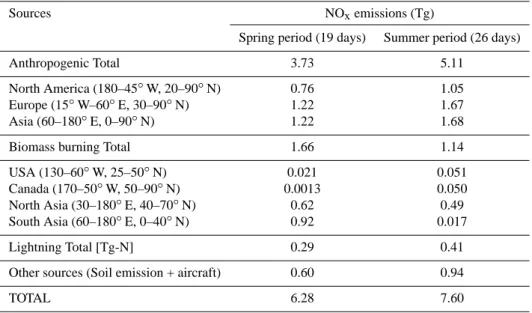
Table 1. Global and regional NOxemission sources used in MOZART-4 simulations for the ARCTAS spring (1–19 April) and summer (18
June–13 July 2008) campaign periods.
Sources NOxemissions (Tg)
Spring period (19 days) Summer period (26 days)
Anthropogenic Total 3.73 5.11
North America (180–45◦W, 20–90◦N) 0.76 1.05 Europe (15◦W–60◦E, 30–90◦N) 1.22 1.67 Asia (60–180◦E, 0–90◦N) 1.22 1.68
Biomass burning Total 1.66 1.14
USA (130–60◦W, 25–50◦N) 0.021 0.051 Canada (170–50◦W, 50–90◦N) 0.0013 0.050 North Asia (30–180◦E, 40–70◦N) 0.62 0.49 South Asia (60–180◦E, 0–40◦N) 0.92 0.017
Lightning Total [Tg-N] 0.29 0.41
Other sources (Soil emission + aircraft) 0.60 0.94
TOTAL 6.28 7.60
Fig. 1. Model NOxsurface emission fluxes during the ARCTAS
spring (1–19 April 2008) and the ARCTAS summer (18 June–13 July 2008) campaign periods.
2004), and of 30 % ± 30 pptv for DC-8 HNO3 (Crounse et
al., 2006). As described in Brock et al. (2011), instrument comparisons were performed during separate coordinated flights with the NASA DC-8 and the NOAA WP-3D at the same altitude. Results from the comparison can be found at: http://www-air.larc.nasa.gov/TAbMEP2 polarcat.html. The preliminary POLARCAT O3 assessment report estimates a
deduced relative bias between the DC-8 and WP-3D instru-ments as the sum of: 0.904 (ppb) + 0.0480*DC-8 O3(ppb)
with the DC-8 taken as an arbitrary reference. The compari-son between DC-8 and WP-3D instruments for HNO3can be
found at: http://www-air.larc.nasa.gov/cgi-bin/ic2008r. The ambient levels reported by the DC-8 instrument during the comparison period were within the reported imprecision of
the WP-3D instrument making it difficult to assess any bias for HNO3between these instruments.
For comparisons between MOZART-4 model simulations and aircraft observations, the MOZART-4 model results from 6-h window averages are sampled along the flight track at the same location, altitude and time of the observations, making use of 1-min average aircraft measurements.
Additional independent comparisons of O3model results
with ground-based FTIR solar absorption measurements are also performed for two sites: Eureka (80◦N, 86◦W) and Thule (77◦N, 69◦W). These measurements were made with Bruker 125 HR FTIR spectrometers, operated in the frame-work of the Netframe-work for the Detection of Atmospheric Com-position Change (NDACC) (Kurylo, 1991; Kurylo and Zan-der, 2000). The retrieval of trace gas profiles from the FTIR spectra are performed using the SFIT2 algorithm, a solar transmittance and retrieval model based on the optimal es-timation method (OEM), and a specific set of microwindows (Batchelor et al., 2009; Hannigan et al., 2009; Lindemaier et al., 2010). The typical total error on the retrieved O3
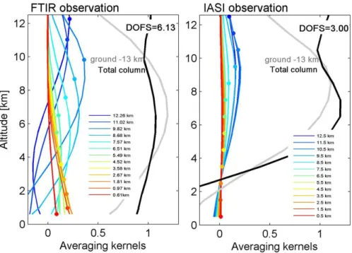
to-tal columns is ∼10 % (Batchelor et al., 2009). During the aircraft campaign periods, measurements at Thule were only available from 1 to 15 April, while a larger set of measure-ments at Eureka were made coinciding with the spring and summer campaigns. Typical FTIR averaging kernels, which express the sensitivity of the retrieval to the abundance of the target species within the layers throughout the atmospheric column, are shown in Fig. 2 (left) for the retrieved tropo-spheric layers and for the tropotropo-spheric and total columns. The analysis of the averaging kernels indicates that most of the retrieved information comes from the measurements.
C. Wespes et al.: Analysis of ozone and nitric acid in spring and summer Arctic 241
Fig. 2. Typical FTIR (left) and IASI (right) O3averaging kernels in partial column units (molecules cm−2/molecules cm−2)for different retrieved layers for O3at Eureka (10 July).
They reveal a DOFS (Degrees Of Freedom for Signal, which represents the pieces of independent information contained in the measurement) ranging from about 5.8 to 6.5 over the spring and the summer campaigns, with a maximum sensi-tivity around 6 km.
O3 profiles from the IASI infrared sounder are also
used here for further comparison with MOZART-4 results. IASI measures the thermal infrared emission of the Earth-atmosphere system between 645 and 2760 cm−1with a field of view of 2 × 2 circular pixels on the ground, each of 12 km diameter at nadir. The IASI measurements are taken at nadir every 50 km along the track of the satellite and they are also taken across-track over a swath width of 2200 km. IASI of-fers in its standard observing mode a global coverage twice a day with overpass times at 09:30 and 21:30 mean local solar time. IASI measures concentrations of several gas-phase species including O3, HNO3, CO, and detects fires
and associated smoke plumes (Clerbaux et al., 2009; We-spes et al., 2009; Coheur et al., 2009; Turquety et al., 2009; Pommier et al., 2010). O3 profiles are retrieved with the
FORLI-O3 (Fast Operational/Optimal Retrievals on Layers
for IASI) processing chain set up by ULB/LATMOS groups (Clerbaux et al., 2009; Dufour et al., 2011). It provides profiles on 39 layers from the surface up to 39 km, rely-ing on a fast radiative transfer and retrieval methodology, based on the Optimal Estimation Method (Rodgers, 2000), which has been developed initially for the retrieval of HNO3
from IASI (Wespes et al., 2009). As described in Scannell et al. (2011), the a priori information (a priori profile and a priori covariance matrix) used for the retrieval of O3is built
from the Logan/Labow/McPeters climatology (McPeters et al., 2007) which is a combination of data from the Strato-spheric Aerosol and Gas Experiment II (SAGE II; 1988– 2001), the Microwave Limb Sounder (MLS; 1991–1999) and data from balloon sondes (1988–2002) to represent the best approximation of the atmospheric state. Note that a sin-gle O3 a priori profile and variance-covariance matrix are
used. The FORLI-O3product is currently under validation,
including polar regions (Scannell et al., 2011; Dufour et al., 2011; Anton et al., 2011). The total error on the retrieval ranges between ∼5 % (Northern latitudes) and ∼15 % (equa-torial latitudes) for the surface-300 hPa column. Only day-time O3IASI observations with a good spectral fit (RMS of
the spectral residual lower than 4 × 10⁻⁸W cm−2sr cm−1) have been used in this study. The reason for only consider-ing the daytime IASI observations relies on a better vertical sensitivity to the troposphere associated with a higher sur-face temperature and a higher thermal contrast (Clerbaux et al., 2009; Boynard et al., 2009). The cloud information from the operational processing is further used for filtering the ob-servations, and only scenes with cloud coverage below 25 % are analyzed (Clerbaux et al., 2009). An example of typical FORLI-O3averaging kernel functions for polar observation
with a DOFS of 3 is represented on the right panel of Fig. 2. The averaging kernels show a maximum sensitivity at around 8 km with a sharp decrease of sensitivity down to the surface, which is inherent to nadir thermal IR sounding in cases of low surface temperature and low thermal contrast. This de-crease of sensitivity, below around 4 km, indicates that the retrieved information principally comes from the a priori at
these altitudes. Taken globally, the DOFS ranges from ∼2.5 in cold polar regions to ∼3.5 at mid-latitudes and up to ∼4.5 in hot tropical region, with a maximum of sensitivity peaking around 6–8 km altitude for almost all situations. For com-parisons with MOZART-4 model simulations, the IASI re-trievals are averaged over the MOZART grid and over the 6-h window of the MOZART-4 outputs.
When comparing model profiles with trace gas retrievals from remote sounders, the high resolution modeled layers must be smoothed using the averaging kernels (A) to be meaningfully compared to the observations. The derived modeled profile is here called xModel Smoothed. In our case,
the MOZART-4 profiles were firstly vertically interpolated to the pressure levels of the a priori profiles (xa)used in the
retrieval algorithms. Then the smoothing of the model pro-files (xModel)to the lower vertical resolution of the
observa-tions (ground-based FTIR or IASI) was performed following (Rodgers, 2000):
xModel Smoothed=xa+A(xModel−xa) (1)
In order to take into account the specific scene of each ob-servation, the averaging kernels of the different observations contained in each MOZART grid have been considered to smooth the gridded MOZART profile.
HNO3 measurements from FTIR and IASI instruments
could not be used here due to a weak sensitivity of these in-struments to this compound in the troposphere (Vigouroux et al., 2006; Wespes et al., 2009).
3 O3and HNO3observations and model evaluation
along the aircraft flight tracks
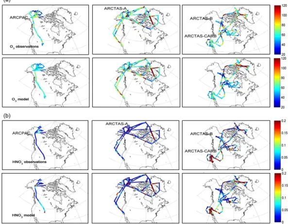
Observed and simulated volume mixing ratio (VMR) of O3
and HNO3along the flight tracks of ARCPAC, ARCTAS-A,
-CARB and -B are shown in Fig. 3. The flight altitudes ex-tend from 0 to 7 km for ARCPAC and from 0 to 12 km for ARCTAS. The highest values observed north of 50◦N both for O3 (red hotspots above 120 ppbv in Fig. 3) and HNO3
(above 0.3 ppbv), principally during ARCTAS, correspond to observations made above 8 km, and show influences from stratospheric air masses. The stratospheric air masses can be diagnosed as [O3]/[CO] > 1.25 (Hudman et al., 2007).
Ex-cluding these, we observe, along the ARCPAC flights, con-centrations ranging from 20 to 90 ppbv for O3, while they
range from 0.01 to 0.12 ppbv for HNO3. For ARCTAS, O3
measurements range from 20 to 120 ppbv and HNO3
mea-surements reach 14 ppb. The maxima for HNO3are observed
over California during ARCTAS-CARB and they can be at-tributed to fires and urban pollution, as further discussed in Sect. 4.1. These observations are broadly consistent with pre-vious measurements in urban plumes (e.g., Emmons et al., 2000; Bey et al., 2001; Neuman et al., 2006).
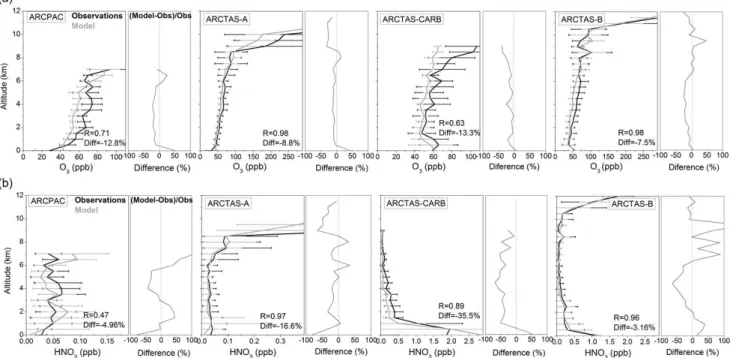
Figure 4 presents the vertical distribution, averaged over 0.5 km layers, of the ARCPAC and the ARCTAS aircraft
ob-servations, along with the model values interpolated to the flight tracks. The differences relative to the observations, ex-pressed as a percentage, are shown on the right panels for each campaign. Vertical distributions of observations and model results show an increase of O3 mixing ratios from
around 50 ppbv at the surface to 90 ppbv in the upper tro-posphere. It is followed by a sharp increase above 8 km for ARCTAS-A and above 11 km for ARCTAS-B, reflect-ing the influence of stratospheric air. The latter is also ob-served in the vertical distributions of HNO3. During the
ARCTAS-CARB and the ARCTAS-B campaigns, a maxi-mum for HNO3 near the surface, followed by a decrease
of VMR with altitude to around 5 km is observed. The highest values near the surface are principally representa-tive of fresh plumes from anthropogenic pollution in addition to fires from California, for the ARCTAS-CARB, and from Canada, for the ARCTAS-B aircraft observations.
The aircraft data set shows the largest variability in the up-per troposphere – lower stratosphere during ARCTAS-A and ARCTAS-B and in the boundary layer for the HNO3
mea-surements during ARCTAS-CARB and ARCTAS-B (hori-zontal bars in Fig. 4). We also find a larger relative variabil-ity associated with the HNO3observations (50–200 %) than
those associated with the O3observations (0–60 %)
consis-tent with the much shorter lifetime of HNO3and to a larger
relative uncertainty in the HNO3 observations (Sect. 2.2).
Relative to the aircraft measurements, the model underesti-mates O3and HNO3concentrations by 5–15 % and 3–35 %
for overall campaign averages, respectively. The relative differences between observations and model are larger for HNO3 (around −80 to 150 %) than for O3 (−40 to 50 %),
possibly explained by the larger variability associated with the HNO3observations that cannot be captured with the
rel-atively coarse model resolution. The high correlation coef-ficients (R) between model and observations, principally for the ARCTAS data sets probably illustrate the large vertical gradient sampled during the aircraft flight tracks and the per-formance of the model for reproducing the variability of ob-servations in space and time. The lower value of R for ARC-PAC data, particularly for HNO3, could result from the lower
vertical gradient sampled during the ARCPAC flights, from the long-distance displacement and smearing of plumes from sources into the Alaskan Arctic, inducing larger model error (Fisher et al., 2010; Rastigejev et al., 2009; Tilmes et al., 2011) and from the large relative uncertainty in the HNO3
observations at concentrations below 0.1 ppbv.
Figure 5 shows a comparison of O3 and HNO3 aircraft
data with MOZART-4 for data representative of the altitude and latitude sampled during the ARCTAS campaign, with the flight altitude plotted on the right axis. In general, the MOZART-4 model reproduces the spatial and temporal vari-ability of observations well. However, some discrepancies can be observed. Extremely low values of O3in the
bound-ary layer in the Arctic (e.g., flights on 8 and 17 April, Fig. 5) are not reproduced in the model. A likely explanation is the
C. Wespes et al.: Analysis of ozone and nitric acid in spring and summer Arctic 243
Fig. 3. (a) O3and (b) HNO3mixing ratios (ppb) observed during the ARCPAC (3 to 23 April 2008), the ARCTAS-A (1 to 19 April 2008)
and the ARCTAS summer (18 June to 13 July 2008) campaigns (ARCTAS-CARB and ARCTAS-B) (top panels) compared to model values (bottom panels) sampled along the flight track at the same time, location and altitude of the observations. The flight tracks extend from 0 to 7 km for ARCPAC, from 0 to 9 km for ARCTAS-CARB and from 0 to 12 km for ARCTAS-A and -B.
missing treatment of the halogen chemistry in MOZART-4, in particular, the bromine chemistry that is responsible for the extreme ozone depletion events that occur within the Arctic boundary layer. Underestimation of HNO3 within the
Arc-tic boundary layer is also simultaneously observed with the overestimation of O3. This probably results from the
mis-representation of the wet deposition processes in the Arctic boundary layer in MOZART-4. The fact that MOZART-4 systematically and simultaneously overestimates O3and
un-derestimates HNO3within the Arctic boundary layer in April
can also be observed in Fig. 4 (lowest 0.5 km). Values of around 100 ppbv or higher observed for O3and higher than
0.5 ppbv for HNO3 along the highest altitude flights (e.g.,
flights on 8, 9 and 17 April, Fig. 5), related to stratospheric air masses, are largely underestimated in the model. This probably results from the coarse horizontal and vertical res-olution of the model results, which dilutes the stratospheric influence, and from the constraint of O3and HNO3and other
long-lived species to a climatology in the stratosphere in MOZART-4 (see Sect. 2.1). For HNO3, other discrepancies
are observed near the surface (between the ground and 2 km)
for flights on 9, 12 and 17 April (see Fig. 5) at Barrow, with a significant underestimation in the model. This suggests that low-altitude transport or subsidence of HNO3-rich air masses
into this region is not well simulated. It is also worth pointing out that most of the variations in both O3and HNO3are
cor-related with the altitude, except for the flight on 13 July near Trinidad Head. This site, which is representative of fresh ur-ban and wildfire plumes in northern California, shows varia-tions that are anti-correlated with the altitude, suggesting fast oxidation of NOxto O3and HNO3in source regions.
As another measure of the model performance, the ra-tio O3/HNO3, can also be compared with that from the
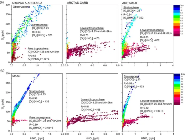
air-craft observations. Figure 6a and b show the O3vs. HNO3
plots for both the aircraft observations and the MOZART-4 results, with the points colored by the altitude of the ob-servations. For ARCPAC and ARCTAS-A (Fig. 6a, left), the [O3]/[HNO3] ratios show, on average, values of 321
for the stratospheric-influenced air masses, diagnosed by [O3]/[CO] ratio larger than 1.25 (Hudman et al., 2007),
while much higher values are observed in the troposphere (4 × 10³). Identically, the ARCTAS-B measurements show a
Fig. 4. Vertical distribution of O3(a) and HNO3(b) ARCPAC and ARCTAS observations averaged over 0.5 km altitude, compared to the
MOZART-4 model values (from 6-h averages). Horizontal bars represent the variability associated with the observations (3σ , where σ is the standard deviation). The differences between the observations and the model are shown on the right panels for each campaign. The correlation coefficient and median of the differences are also indicated.
Fig. 5. (a) O3and (b) HNO3observations along the track of seven flights representative of the altitude and the latitude sampled during
ARCTAS (dark grey dots). The MOZART-4 results (from 6-h averages) are interpolated to the flight path (from 1-min averages) (black line). The flight altitude (thin grey line) is plotted against the right axis.
high [O3]/[HNO3] ratio (5 × 10³)in the free troposphere (not
shown), while a ratio of 322 is measured in higher-altitude stratospheric air. However, below 2 km, averaged ratios of 453 and 652, respectively observed during ARCTAS-CARB
and ARCTAS-B, with values as low as 8, indicate weaker ozone production despite the rapid removal of HNO3by
de-position in the boundary layer. These particular lower values characterize fresh air masses from North American urban and
C. Wespes et al.: Analysis of ozone and nitric acid in spring and summer Arctic 245
Fig. 6. O3vs. HNO3from ARCPAC and ARCTAS-A (left), ARCTAS-CARB (middle) and ARCTAS-B (right) observations (a) compared
to the MOZART-4 results (b), with points colored by altitude (in km) of observations.
fire emissions (Californian for ARCTAS-CARB and Cana-dian for ARCTAS-B) corresponding to the highest concen-trations of HNO3illustrated in Fig. 3. This is consistent with
earlier studies which point to different HNO3vs. O3
relation-ships in the troposphere and in the stratosphere (Bregman et al., 1995; Talbot et al., 1997; Schneider et al., 1999; Neuman et al., 2001; Popp et al., 2009) and which show lower ozone production for air masses with fresh emissions from biomass burning and urban sources than in the free troposphere (Shon et al., 2008). For each specific air mass (fresh pollution, free troposphere or stratosphere-contaminated air mass) and for each data set, we find that O3/HNO3 ratios and the scatter
values are of comparable magnitude between the aircraft ob-servations and the model results. Ratios as low as 8 below 2 km are well reproduced by the model. The largest differ-ences between the ratios from observations and from model are observed for ARCTAS-CARB. They are driven by a too high formation of HNO3in the lowermost layer coinciding
with an underestimation of O3, as indicated in the Figs. 4 and
5. Some discrepancies in the model are also identified for the stratosphere-contaminated air masses: the ARCTAS-A ob-servations show a relatively broad O3/HNO3relationship in
comparison with the observations during ARCTAS-B. This presumably reflects different dynamical and photochemical
histories of the air masses sampled by the aircraft during the spring, when the stratosphere is dynamically active, and during the summer; characterized by a more uniform photo-chemical history associated with summertime easterly flow and very little stratospheric wave activity. The differences in the compactness between the modeled and the observed stratospheric O3/HNO3relationship can be attributed to the
missing stratospheric chemistry and the use of climatological values in the stratosphere (see Sect. 2.1).
4 Source attribution of O3and HNO3 Arctic pollution
during spring and summer 2008
In this section, we use MOZART-4 model simulations to diagnose the contributions from the individual sources to the O3 and HNO3 profiles. As described in Lamarque et
al. (2005) and Pfister et al. (2006, 2008), the amount of O3
or HNO3produced from the different NOxemission sources
is quantified by tagging the NO emissions. The tagged NO (from the emissions shown in Fig. 1) is traced through the hydrocarbon and CO oxidation and through all the odd nitro-gen species (HNO3, PAN, N2O5, organic nitrates, etc.) to
ac-count for recycling of NOx. The tagged O3and HNO3result
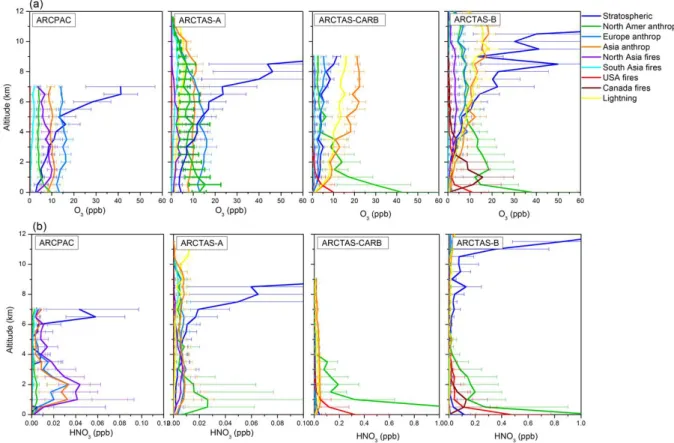
Fig. 7. Vertical distributions of O3 (a) and HNO3(b) source contributions from MOZART-4 simulations along the flight tracks of the ARCPAC, ARCTAS spring and summer deployments. Data are averaged over 0.5 km layers and tagged by source type and region. Horizontal bars represent the variability associated with each tagged contribution (3σ , where σ is the standard deviation).
Emmons et al. (2010b, 2011), this tagging technique is addi-tive. The sum of the tagged species resulting from each NOx
source tagged separately reproduces within a few percent the tagged species from the total NOxemissions.
4.1 Partitioning along the aircraft flight tracks
Figure 7 presents the vertical distributions of O3and HNO3
concentrations from the MOZART-4 simulations along the ARCPAC and ARCTAS flight tracks for different source types and regions: stratospheric, anthropogenic (North American, European and Asian), biomass burning (North Asian, South Asian, American and Canadian) and lightning-produced NOx. For both the ARCPAC and ARCTAS-A
cam-paigns, the mean concentrations of O3are dominated by
Eu-ropean anthropogenic emissions at low altitude. They are followed by North American and Asian anthropogenic con-tributions for the ARCTAS-A measurements, while the AR-CPAC measurements contain large contributions from Asian anthropogenic emissions and from North Asian fires. The latter, which reflects intense Russian fires, is much weaker along the ARCTAS-A than along the ARCPAC flight tracks (Fisher et al., 2010), while the North American anthro-pogenic contribution is much larger along the ARCTAS-A
than along the ARCPAC fight tracks. This reflects the dif-ferent sampling strategies between the two campaigns (Ja-cob et al., 2010; Brock et al., 2011). Transport from the stratosphere, which is responsible for a large enhancement of tropospheric ozone in regions of subsidence (Cooper et al., 2002; Liang et al., 2009), is the predominant source above 5 km. It becomes even larger than the sum of the tropo-spheric contributions above 8 km. During ARCTAS-A, the mean concentrations of HNO3are dominated at low altitude
by the North American anthropogenic contribution, while they are dominated by the Russian fires contribution during ARCPAC. Transport of anthropogenic HNO3 from Europe
and from Asia into the Arctic is lower in comparison with that of ozone. This can be explained by a shorter lifetime of HNO3in the lower layers (a few hours) compared to that of
O3(a few days). Above 5 km, transport from the stratosphere
dominates the HNO3distributions.
During the ARCTAS-CARB and the ARCTAS-B cam-paigns, the stratospheric influence on tropospheric ozone and nitric acid is less pronounced than during the spring. This is due to weaker stratosphere-troposphere exchanges during the summer but also to the lower latitudes sampled during ARCTAS-CARB. For both O3and HNO3, the anthropogenic
C. Wespes et al.: Analysis of ozone and nitric acid in spring and summer Arctic 247
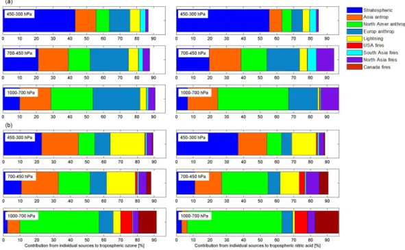
Fig. 8. Partitioning of principal sources of O3(left) and HNO3(right) in altitude bands of ground-700 hPa, 700–450 hPa and 450–300 hPa along the ARCTAS spring (a) and summer (b) flight tracks (from 18 June to 13 July), as simulated by MOZART-4, expressed in percentage (%) of the total.
contribution from North America shows a strong maximum in the lowest layers. Contribution from intense North Amer-ican fire emissions (California and/or Canada) also shows an important impact on tropospheric ozone in the boundary layer. Evidence for enhanced ozone in boreal fires plumes during the ARCTAS-B campaign has already been reported in Alvarado et al. (2010). We also observe, especially for O3, an increasing contribution in the summer months from
lightning-produced NOxand from Asian anthropogenic
pol-lution with altitude. The latter is in agreement with the fact that trans-Pacific transport of Asian ozone pollution mainly takes place in the free troposphere where the ozone lifetime is longer (several months) and the winds are strong (Liang et al., 2004; Price et al., 2004). Note also that, based on the model bias relative to the aircraft observations (see Sect. 3), less confidence should be attributed to the quantitative par-titioning of the smallest contributors to tropospheric O3and
HNO3.
For both O3 and HNO3 during ARCTAS-A/B, North
American anthropogenic pollution sources dominate the variability in the lower troposphere indicating direct low-altitude transport into the Arctic. The ARCPAC variability is principally determined by the Russian fires emissions and the European anthropogenic pollution. Transport from the stratosphere dominates the variability in the higher altitudes. We also found that the model captures the vertical gradient in the variability (see Sect. 3, Fig. 4) but it underestimates the variability range. When separating data by anthropogenic,
stratospheric or fires influence, we found that the underesti-mation of O3and HNO3concentrations in the lower/middle
altitudes in the model (see Sect. 3, Fig. 4) is principally dom-inated by an underrepresentation of local pollution sources (North American anthropogenic pollution, Californian and Canadian fires) during ARCTAS, while it is attributed to an underrepresentation of Russian fire emissions, Asian and Eu-ropean anthropogenic pollution during ARCPAC. At higher altitudes, for the ARCPAC, ARCTAS-A/B observations, the underestimation is related to an underrepresentation of the stratospheric influence. The underrepresentation of both modeled concentrations and variability are possibly due to a mix of uncertainties introduced by the coarse grid of the model leading to too much diffusion, problems in the trans-port of fine-scale plumes in the model, uncertainties in the emissions, possible bias in the NOypartitioning, incomplete
stratospheric chemistry of MOZART-4 and interpolation of the MOZART-4 results (from 6-h averages) to the flight path (1-min averages).
In order to further illustrate the tagged contributions to tro-pospheric O3 and HNO3, Fig. 8 represents the partitioning
by source type and region over three altitude ranges during the ARCTAS spring and summer campaigns, as simulated by MOZART-4. Differences between total simulated O3or
HNO3(100 %) and the sum of tagged contributions are
prin-cipally due to NOxemissions from soils, but also from
air-craft and from ships. An interesting feature in Fig. 8 lies in the observation of increasing relative contribution, during
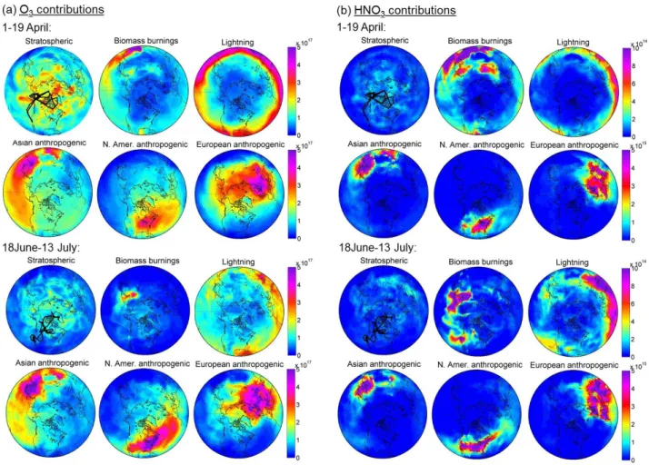
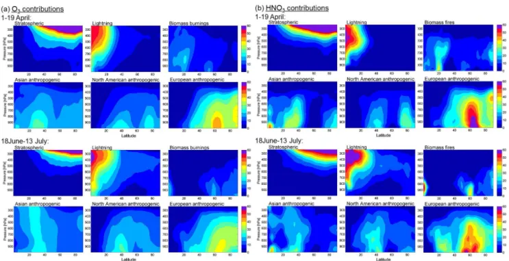
Fig. 9. Principal contributions to O3(a) and to HNO3(b) columns (molecules cm−2)from the ground to 300 hPa during spring (from 1
to 19 April) and summer (from 18 June to 13 July) ARCTAS campaigns, as simulated by MOZART-4. The flight tracks corresponding to these periods are superimposed in black on the stratospheric contribution plots. Note that the color scales for anthropogenic contributions to HNO3are different than for the other sources.
the summer, from Asian anthropogenic pollution with alti-tude for HNO3. The partitioning from that source is larger
than from other anthropogenic individual sources (American and European) at higher altitudes, suggesting that this source tends to favor HNO3 in the upper troposphere where it is
longer lived (several weeks to a month), making it a can-didate for the transport of pollution (Miyazaki et al., 2003; Neuman et al., 2006). It is also worth pointing out that, both during the summer and the spring, the relative partitioning of O3and of HNO3are similar along the flight tracks of the
air-craft missions, reflecting the chemical link between the two compounds.
4.2 Partitioning over the Arctic (north of 60◦N)
Figure 9 shows simulated spring and summer O3 and
HNO3columns from the ground to 300 hPa, of each tagged
tracer over the Northern latitudes. Asian, European and North American anthropogenic pollution are of comparable
magnitude (reaching 5 × 10¹⁷ and 5 × 10¹⁵molecules cm−2 respectively for O3 and for HNO3), but with distinct
geographical signatures. Sources in Europe dominate in the European sector of the Arctic over Scandinavia (4 × 10¹⁷molecules cm−2 on average for O3) reflecting
northward transport, and in the Asian sector of the Arc-tic (3 × 10¹⁷molecules cm−2 on average for O3)through a
westerly trans-Siberian transport pathway. Pollution from North America contributes only a small amount to the Arc-tic pollution (around 1.5 × 10¹⁷molecules cm−2 on
aver-age for O3). According to the ARCPAC observations,
the Asian and the European influences dominate the pol-lution over Alaska. Relative to anthropogenic O3, which
shows horizontally smoothed distributions, anthropogenic HNO3 presents a strong horizontal gradient overall the
tro-posphere. This difference is probably due to washout or to the uptake of HNO3 on dust or ice (Querol et al.,
2008; Zhang et al., 2008), making it shorter-lived than O3
C. Wespes et al.: Analysis of ozone and nitric acid in spring and summer Arctic 249
Fig. 10. Vertical and latitudinal distributions of the relative contributions (%) to O3(a) and HNO3(b) concentrations during the spring (from 1 to 19 April) and summer (from 18 June to 13 July) ARCTAS campaigns, as simulated by MOZART-4.
As a result, the anthropogenic emissions contribute only slightly to the Arctic background concentrations of HNO3
(5 × 10¹⁴molecules cm−2). Even though they were partic-ularly intense during the spring campaigns, the Southeast Asian fires show only a small influence on the Arctic due to the low latitude of the emissions. During the summer, Russian fire emissions greatly contribute to the tropospheric columns over Eastern Siberia (3 × 10¹⁷molecules cm−2 for O3 and 1.5 × 10¹⁵molecules cm−2 for HNO3) with some
contributions over the American sector of the Arctic. Emissions from Californian fires are also observed. Fi-nally, lightning which principally occurs at the equato-rial belt also has a non-negligible contribution to the tro-pospheric columns of O3 (1 × 10¹⁷molecules cm−2) and
HNO3 (1 × 10¹⁵molecules cm−2)in the Arctic principally
during the summer.
Figure 10 presents the vertical and latitudinal distribu-tions of the most important contributors to O3 (Fig. 10a)
and HNO3 (Fig. 10b) for the spring and the summer
pe-riods, as simulated by MOZART-4. Consistent with stud-ies of CO during ARCTAS (Fisher et al., 2010; Tilmes et al., 2011), anthropogenic pollution dominates concentra-tions over the Northern Hemisphere between the surface and 400 hPa, through lifting to the middle troposphere and trans-port towards higher latitudes. The European contribution particularly dominates throughout the Arctic, reaching up to 45 % and 60 % of the total abundance of O3and HNO3,
re-spectively. The Asian emissions are dominant below 40◦N with a contribution of 35 % for O3 and HNO3. They reach
up to 20 % of the Arctic background via uplift and transport associated with warm conveyor belts (WCBs) over China (Stohl, 2006). The much smaller North American emis-sions, which also involve uplift in WCBs, make a limited contribution to the Arctic concentrations of 20 % between the surface and 700hPa. The influence of the biomass burn-ing emissions on the Arctic composition, with a contribution of around 15 % on average for O3and HNO3, results
princi-pally from the Siberian fires (maxima at 55–60◦N) occurring during spring and summer. The large fires in the Southeast Asian region in April (maxima at 20–30◦N) have a mini-mal impact on the Arctic abundances. Their contribution is smaller than the Asian anthropogenic contribution, even in the upper troposphere where it results from transport with WCBs (Bey et al., 2001). Subsiding stratospheric air masses dominate concentrations at pressure less than 400 hPa into the Arctic, where they exceed 60 % of O3 or HNO3
Arc-tic abundance. During April, transport from the stratosphere shows a contribution of around 10 % down to the boundary layer. Contributions from lightning to the Arctic composi-tion during April are relatively small, even at high altitude. During summer, they reach up to 20 % of the O3or HNO3
Arctic background concentrations at 400–500 hPa with some descent (10 %) down to the surface. It is also worth noting that, as previously discussed, the principal differences be-tween the distributions of O3and HNO3lie in a deeper
hori-zontal and vertical gradients for HNO3concentrations.
Moreover, it is interesting to indicate that the partition-ing based on the aircraft track flights (Fig. 8) is generally
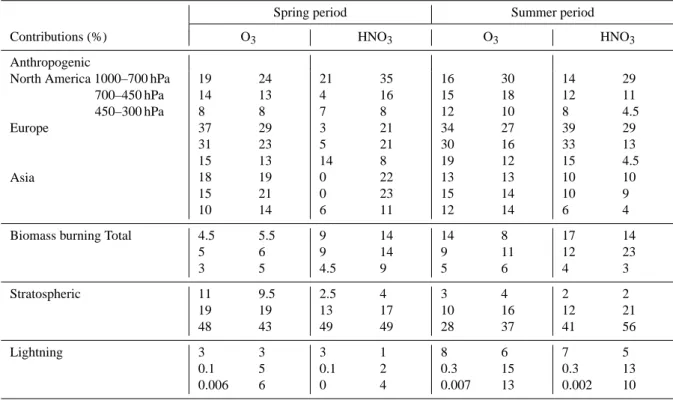
Table 2. Contribution, expressed in percentage (%) of the total, of the principal sources of O3and HNO3in altitude bands of ground-700 hPa,
700–450 hPa and 450–300 hPa, based on the aircraft sampling (>60◦N) and for the entire Arctic (>60◦N) for the spring and the summer phases of the ARCTAS campaigns, as simulated by MOZART-4.
Spring period Summer period
Contributions (%) O3 HNO3 O3 HNO3
Anthropogenic
North America 1000–700 hPa 19 24 21 35 16 30 14 29 700–450 hPa 450–300 hPa Europe Asia 14 8 37 31 15 18 15 10 13 8 29 23 13 19 21 14 4 7 3 5 14 0 0 6 16 8 21 21 8 22 23 11 15 12 34 30 19 13 15 12 18 10 27 16 12 13 14 14 12 8 39 33 15 10 10 6 11 4.5 29 13 4.5 10 9 4 Biomass burning Total 4.5
5 3 5.5 6 5 9 9 4.5 14 14 9 14 9 5 8 11 6 17 12 4 14 23 3 Stratospheric 11 19 48 9.5 19 43 2.5 13 49 4 17 49 3 10 28 4 16 37 2 12 41 2 21 56 Lightning 3 0.1 0.006 3 5 6 3 0.1 0 1 2 4 8 0.3 0.007 6 15 13 7 0.3 0.002 5 13 10
Left: for the entire Arctic (>60◦N)
Right: based on aircraft sampling (>60◦N)
different from that for entire Arctic (Fig. 10), except for mid-dle/upper tropospheric O3, which is longer-lived and better
mixed than HNO3. Table 2 summarizes the contribution of
the principal sources based on the aircraft sampling and for the entire Arctic, for the spring and the summer phase of the ARCTAS campaigns. The aircraft sampling patterns are ob-served to influence the partitioning analysis, with an over-representation of the North American anthropogenic contri-bution (∼10 % for O3and ∼15 % for HNO3on average) and
an underrepresentation of the European anthropogenic con-tribution (∼10 % for O3 and ∼17 % for HNO3on average)
in the lower/middle troposphere, in comparison with parti-tioning from the entire Arctic. The overestimation of the biomass burning contribution to lower/middle tropospheric HNO3, based on aircraft sampling patterns, reflects the
in-fluence from intense Asian fires in addition to the impact of Canadian fires during the summer. The lightning tion over all the troposphere and the stratospheric contribu-tion in the middle/upper troposphere for the summer period are also influenced by the aircraft sampling patterns.
5 Tropospheric O3observed by FTIR and IASI during
ARCTAS
In this section, we test the ability of the FTIR and IASI in-struments to observe the long-range transport of pollution into the Arctic by investigating the daily variability of O3
measurements from IASI and from FTIR at Eureka (80◦N, 86◦W) and at Thule (77◦N, 69◦W) in comparison with the MOZART-4 results previously evaluated in Sect. 3. Based on an IASI sensitivity analysis, we consider, in this section, tropospheric columns between ground and 300 hPa both to limit as much as possible the stratospheric and the tropopause height variation influence and to contain the altitude range of maximum sensitivity in the troposphere (see Sect. 2.2). We also make a further use of the tagged tracers to assist in the interpretation of the O3variability observed by these
instru-ments.
5.1 FTIR observations of Arctic pollution
Figure 11 (top) shows the comparison of model results with observations of daily mean O3 columns from ground to
300 hPa, from FTIR observations at Eureka and at Thule during spring and summer 2008. For the purpose of the
C. Wespes et al.: Analysis of ozone and nitric acid in spring and summer Arctic 251
Fig. 11. Top: daily mean O3columns from ground to 300 hPa at Thule (left) for 1 to 15 April 2008 and at Eureka (right) for 1 April to 13 July
2008. The ground-based FTIR measurements (black) are compared to raw model values (red) and smoothed (blue) with the FTIR averaging kernels. Vertical bars represent the daily variability associated with the tropospheric columns (3σ , where σ is the daily standard deviation). The correlation coefficient and median of the differences between the observations and the model (calculated as [(model-obs.)/obs.]·100 %) are also indicated. Bottom: contributions of principal sources to O3tropospheric columns over Thule (left) for 1 to 15 April 2008 and Eureka
(right) for 1 April to 13 July 2008, smoothed with the FTIR averaging kernels.
comparison, MOZART-4 results have been smoothed by the FTIR averaging kernels (see Sect. 2.2, Fig. 2). Comparison of measurements with model results shows good agreement within 1 × 10¹⁷molecules cm−2, with a negative bias within −15 % on average. This can be explained by the underes-timation of model results of around 5–15 % as discussed in Sect. 3, by the retrieval total errors (Sect. 2.2) and by the daily variation associated with the FTIR observations (verti-cal bars in Fig. 11).
Similarly to the partitioning analysis along the flight tracks (Sect. 4.1), MOZART-4 simulations have been used to sim-ulate the FTIR tropospheric O3contributions from the
prin-cipal sources: stratospheric, anthropogenic, biomass burning and lightning (Fig. 11, bottom). Following the formalism of Rodgers (2000) (Eq. (1), Sect. 2.2), it can be shown that:
xModel Smoothed=xa+A[(6xTracer) −xa] (2)
where xTracerrepresents the profile from each tagged
contri-bution. This expression can be separated into two compo-nents: one representing the contributions from each tracer smoothed by the averaging kernels, calculated as A(xTracer),
and the second, the a priori contribution, representing the contribution from the a priori to the retrieved tropospheric columns, due to the limited vertical sensitivity of the instru-ment. It is calculated as xa−A(xa).
The observations at Thule and Eureka are dominated by the anthropogenic contribution, followed by the stratospheric influence (Fig. 11, bottom). At Thule, the anthropogenic pollution represents, on average, 54 % of total concentra-tion (23 % from North America, 18 % from Europe and 12 % from Asia), the stratospheric fluxes count for 21 % and
light-ning for 5 %. Some contribution from biomass burlight-ning is also likely affecting the FTIR measurements to a weak extent (less than 4 %). The small fraction from the a priori informa-tion (only 1.2 %) reflects a high vertical sensitivity through-out the troposphere. The differences between the total simu-lation and the sum of the tagged contributions (around 15 % on average) can be attributed to the contribution from soils and aircraft emissions. The day-to-day variability observed at Thule can mainly be attributed to the day-to-day variability associated with the stratospheric flux of ozone, which shows an amplitude of 3 × 10¹⁷molecules cm−2.
At Eureka, the contributions are identified as follows: 52 % from the anthropogenic sources (14 % from North America, 23 % from Europe and 14 % from Asia), 20 % from the stratospheric flux, smaller influence from biomass fires (9 %) and from lightning (6 %) and a negligible a pri-ori contribution (1 %). The stratospheric and the anthro-pogenic sources have the most variability, with amplitudes of 3 × 10¹⁷molecules cm−2 and 2 × 10¹⁷molecules cm−2 re-spectively. The anthropogenic source amplitude over the campaign periods shows up as a decrease in the summer while the stratospheric source is strongly variable on a daily basis, though being also much less in summer as compared to spring. As discussed in Sect. 4.2, the contributions from lightning to the Arctic composition are small during April, but they are as large as 18 % during the summer. The most elevated concentrations from fires over May and June with contributions reaching up to 20 % principally result from the Siberian emissions.
Fig. 12. Same as Fig. 11 but for comparison with IASI satellite measurements within the 1.4◦×1.4◦MOZART-4 grid around Thule (left) or Eureka (right).
5.2 IASI observations of Arctic pollution
Figure 12 is similar to Fig. 11, but for the IASI observations extracted within the MOZART grid box around Thule or Eu-reka. Here, MOZART-4 results have been smoothed by the IASI averaging kernels (see Sect. 2.2, Fig. 2). Comparison of the measurements with model results shows an agreement within 1–2 × 10¹⁷molecules cm−2on average, which corre-sponds to a negative average bias of around −15 %. It prob-ably reflects, on one hand, the tendency of IASI retrievals to overestimate the tropospheric ozone columns by ∼10 % in the Northern latitudes (Boynard et al., 2009), and, on the other hand, the underestimation of the concentrations from MOZART-4 in these latitudes (see Sect. 3). It also can be largely explained by the IASI daily variations (3σ values of ∼6 × 10¹⁷molecules cm−2on average).
Contrary to the FTIR observations, the observations from IASI at Thule and Eureka are dominated by the stratospheric contribution. This results from a higher sensitivity of IASI in the higher layers where the stratospheric influence represents the largest contributions (Figs. 7 and 10). This also makes the underrepresentation of the stratospheric influence in the model (reaching 25 %, as previously discussed when com-paring aircraft data and model results in Sect. 3) largely re-sponsible for the differences between the IASI observations and the model results. The IASI measurements are also more affected by the a priori information than the ground-based FTIR measurements, because of a lower vertical sensitivity of IASI in the lowest layers. As a consequence, IASI detects smaller contributions from anthropogenic pollution and fires than the FTIR instruments.
At Thule, the stratospheric and the anthropogenic contri-butions represent, on average, 53 % and 14 % of the total concentration (with 5.5 % from North America, 4.5 % from Europe and 4.0 % from Asia) respectively. The a priori
infor-mation contributes importantly with 22 % over the entire tro-posphere. The contribution from fires, mainly from Siberia, and from lightning is significantly weaker (less than 3.5 % each on average). Contributions of 6 % from soils and air-craft emissions were calculated. The day-to-day variabil-ity can mainly be attributed to the variabilvariabil-ity of the ozone stratospheric contribution, which shows large amplitudes up to 3 × 10¹⁷molecules cm−2, as indicated by the MOZART-4 simulations.
At Eureka, the stratospheric influence is again the most important (46.1 % on average) decreasing over the sum-mer. The relative contribution from the anthropogenic sources accounts for 17 % (5.5 % from North America, 6.5 % from Europe and 5.0 % from Asia). The a pri-ori contribution represents a fraction of 19 %. Influ-ences from fires and from lightning contribute to the Eu-reka background concentration with a fraction smaller than 4.5 % each. Both the stratospheric and the anthropogenic sources have the maximum variability, with amplitudes of 3 × 10¹⁷molecules cm−2 and 2 × 10¹⁷molecules cm−2
re-spectively. It is also worth pointing out that IASI retrievals at Thule and at Eureka are characterized by a sharp decrease of the a priori contribution between April and July observations, with contributions ranging from 3 × 10¹⁷molecules cm−2 to 5 × 10¹⁶molecules cm−2. The larger contribution dur-ing the sprdur-ing reflects a lack of sensitivity probably due to both smaller thermal signal above ice-covered surfaces and smaller thermal contrast in the cold boundary layers.
In order to further test the ability of IASI to observe the transport and the variability over the scale of the Arctic, Fig. 13 shows the mean O3columns from ground to 300 hPa
during the ARCTAS spring and summer periods as observed by IASI and compared to MOZART-4 model values. The horizontal distributions of the Northern latitude concentra-tions show similar patterns between the observaconcentra-tions and the
C. Wespes et al.: Analysis of ozone and nitric acid in spring and summer Arctic 253
Fig. 13. Mean O3columns (×1017molecules cm−2)from ground to 300 hPa during the spring (from 1 to 19 April) and summer (from
18 June to 13 July) campaign periods, observed by the IASI satellite instrument and simulated by MOZART-4, smoothed according to the averaging kernels of the IASI observations. The percent differences between the observations and the model results (calculated as [(model-obs.)/obs.]·100 %) are shown on the right panel.
simulations. During the spring, both IASI and MOZART-4 show highest concentrations over the Arctic, while during the summer, the highest values are observed above south-west Asia. Observations and model datasets are reasonably well correlated (R = 0.79 during the spring and R = 0.88 during the summer campaign periods) and the mean relative differ-ences (4.1 ± 39.4 % and −4.4 ± 29.9 %, respectively for the two periods) indicates the absence of a systematic bias be-tween the model and the observations. The high differences (averaged negative bias of around 20 %) observed over the Arctic can be explained by the underestimation of the strato-spheric contribution in the model (as previously discussed for observations at Eureka and at Thule), while the aver-aged positive bias (around 20 %) measured at low latitudes could be mostly attributed to the tendency of MOZART-4 to overestimate the O3 concentrations in the Northern Tropics
(Emmons et al., 2010a) and to larger total retrieval errors on the IASI tropospheric columns, principally found at the in-tertropical latitudes (∼15 % on average, Sect. 2.2). These larger total errors are possibly due to the stronger impact of the water vapor lines on O3 retrievals at these latitudes
(Hurtmans et al., 2011). Dilution on the model spatial scale (∼140 km) compared to IASI spatial scale (∼12 km at nadir)
could also explain a part of the differences. These differences lead to a stronger latitudinal gradient from IASI observations in comparison to that from the model.
Figure 14 shows O3columns from ground to 300 hPa as
observed by IASI and modeled by MOZART-4 during two specific episodes of pollution transport across the Arctic: 14–16 April during the spring campaign and 2–5 July dur-ing the summer campaign. Principal contributions (strato-spheric, anthropogenic, fires and lightning) as simulated by the model and smoothed using the IASI averaging kernels are also shown for the purpose of our analysis. Both IASI and MOZART-4 show elevated columns over Northern lati-tudes. Based on modeled source contributions, this enhance-ment reflects principally a strong stratospheric influence dur-ing the sprdur-ing, while it mainly results from a mix of an-thropogenic pollution from Europe, Asia and North Amer-ica during the summer. Similar to the analysis presented in Sect. 4.2., the highest values for anthropogenic pollution (up to 7 × 10¹⁷molecules cm−2)are observed over the European sector of the Arctic during the two periods (a contribution of ∼50 % to the tropospheric column), followed by maxima of 5 × 10¹⁷molecules cm−2 over the Asian and the American sectors (see Sect. 4.2). Large anthropogenic plumes from
Fig. 14. Mean O3columns (molecules cm−2)from ground-300 hPa, over 14–16 April and 2–5 July periods observed by the IASI satellite
instrument and simulated by MOZART-4 smoothed according to the averaging kernels of IASI observations. Contributions of principal sources to O3tropospheric columns as modeled in MOZART-4 and smoothed with the IASI averaging kernels are also shown.
Europe to Asia through a westerly trans-Siberian transport pathway, from eastern Asia across the Pacific and from east-ern USA across the Atlantic are clearly shown in the distribu-tions. This example illustrates the ability of IASI to observe anthropogenic outflow transported over a long distance and reaching the Arctic border. However, evidence of enhanced ozone from a mix of anthropogenic pollution is not clearly detected from the anthropogenic contribution smoothed us-ing the IASI averagus-ing kernels. This results from a sharp decrease of the IASI vertical sensitivity in the middle/lower troposphere above these cold ice-covered surfaces even dur-ing the summer time. This lack of vertical sensitivity over the Arctic leads to a collar region of enhanced anthro-pogenic ozone circling the colder Arctic, in contrast to the non-smoothed MOZART-4 anthropogenic tag (see Sect. 4.2, Fig. 9). This collar region is characterized by DOFS larger than 3.2 while colder Arctic surfaces show lower DOFS. This threshold DOFS value of ∼3.2 indicates the mini-mum sensitivity required for the detection of anthropogenic ozone into the Arctic. Principally during April, evidence for biomass burning emissions from eastern Asia (reaching concentration of 3 × 10¹⁷molecules cm−2, ∼30 % of
tropo-spheric columns) with some transport to higher latitudes are also detected in the IASI measurements. Finally, some con-tributions from lightning to tropospheric O3as observed by
IASI are also detected in higher latitudes principally dur-ing the summer with values of ∼1 × 10¹⁷molecules cm−2 (reaching 15 % of the tropospheric columns).
6 Conclusions
O3and HNO3observations from the NASA ARCTAS and
NOAA ARCPAC aircraft campaigns provide information of the sources of pollution into the Arctic during spring and summer 2008.
The MOZART-4 model generally reproduces the vari-ability of observations in space and time for both O3 and
HNO3, especially during ARCTAS. During ARCPAC, the
long-distance displacement and smearing of plumes from sources into the Alaskan Arctic seems to introduce larger model error. The model underestimates both O3and HNO3
concentrations by 5–15 % and 3–35 %, respectively. For the ARCTAS measurements, the underestimation of O3and
HNO3concentrations is attributed to an underrepresentation
of both anthropogenic sources and stratospheric influence. During ARCPAC, the underestimation is tied to an under-representation of anthropogenic sources and Russian fires emissions. The O3/HNO3ratio characterizing different air
mass types (fresh plumes, free troposphere and stratosphere-contaminated air masses) are well reproduced in the model. The largest differences between observations and model are observed in the freshly polluted plumes of the ARCTAS-CARB and the ARCTAS-B campaigns, pointing to the prob-able impact of the coarse model resolution and the associ-ated diffusion on O3production in polluted regions. In
sum-mary, the underestimation of concentrations in the model could result from a mix of uncertainties in emission inven-tories, underestimation of the stratospheric influence, trans-port errors in the model introduced by too much diffusion due to the coarse resolution of the model and interpolation