HAL Id: insu-02075668
https://hal-insu.archives-ouvertes.fr/insu-02075668
Submitted on 21 Mar 2019
HAL is a multi-disciplinary open access
archive for the deposit and dissemination of
sci-entific research documents, whether they are
pub-lished or not. The documents may come from
teaching and research institutions in France or
abroad, or from public or private research centers.
L’archive ouverte pluridisciplinaire HAL, est
destinée au dépôt et à la diffusion de documents
scientifiques de niveau recherche, publiés ou non,
émanant des établissements d’enseignement et de
recherche français ou étrangers, des laboratoires
publics ou privés.
Natron’s saline mudflats
Lieven Clarisse, M. van Damme, W. Gardner, P.-F. Coheur, Cathy Clerbaux,
S. Whitburn, Juliette Hadji-Lazaro, Daniel Hurtmans
To cite this version:
Lieven Clarisse, M. van Damme, W. Gardner, P.-F. Coheur, Cathy Clerbaux, et al.. Atmospheric
ammonia (NH3) emanations from Lake Natron’s saline mudflats. Scientific Reports, Nature Publishing
Group, 2019, 9, pp.4441. �10.1038/s41598-019-39935-3�. �insu-02075668�
Atmospheric ammonia (NH
3
)
emanations from Lake Natron’s
saline mudflats
L. Clarisse
1, M. Van Damme
1, W. Gardner
2, p.-F. Coheur
1, C. Clerbaux
3,1, s. Whitburn
1,
J. Hadji-Lazaro
3& D. Hurtmans
1In a recent global analysis of satellite-derived atmospheric NH3 data, a hotspot was observed in the
vicinity of Lake Natron, tanzania. the lake is in the centre of an endorheic (limited drainage) basin and has shallow, saline-alkaline waters. Its remote location and the absence of nearby large anthropogenic sources suggest that the observed NH3 is mainly of natural origin. Here we explore 10 years of IASI
NH3 satellite data and other publicly available datasets over the area to characterize the natural NH3
emissions in this unique ecosystem. temporal analysis reveals that the emissions are episodic and linked with the lake’s surface area. the largest NH3 column loadings generally occur at the end of the dry season
in September–November over Lake Natron’s largest mudflat, that is exposed with receding water levels. The timing is different from the agricultural dominated NH3 emissions in the wider Natron area, which
peak early in the year, after the first wet season. The likely source of NH3 at Lake Natron is decomposition
of organic material, either from rivers and springs or produced in the lake (plankton, bird excreta). High temperatures and alkalinity are known to promote NH3 losses from soda lakes. We formulate six
processes that may explain why the largest losses are observed specifically over concentrated brines and/ or exposed sediments. As a by-product, we also show that hyperspectral infrared sounders such as IAsI are capable of mapping different types of evaporative minerals such as trona and thermonatrite.
Ammonia (NH3) plays a critical role in the global biogeochemical cycle of nitrogen1 as one of the key components
of reactive nitrogen. Largely due to the widespread availability of industrially fixed nitrogen2, atmospheric emis-sions of NH3 are increasing steadily3,4, with devastating effects on air quality, ecosystems and climate5. Sources of
atmospheric ammonia include animal waste, fertilizers, combustion (biomass burning, waste burning, transport), industry (production of chemicals, manufacturing processes), soils, plants and oceans3,6,7.
About a decade ago, it was discovered that infrared satellites can detect and measure atmospheric NH3, which
resulted in the first measurement-based global maps of its distribution8. Satellite measurements are currently available from four instruments: AIRS9, TES10, CrIS11 and IASI12. Recently13, a hyperresolved (0.01° × 0.01°) world map of NH3 was presented, following the combined exploitation of all available IASI satellite data over
ten years and a series of algorithmic improvements14. Careful analysis of this map revealed 248 NH
3 emission
hotspots. About one third of these hotspots were attributed to high-density animal farming, but surprisingly, the majority were linked to industrial activity, in particular to chemical fertilizer production plants.
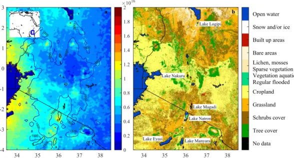
The hotspot over Lake Natron, Tanzania (Figs 1 and 2) was the only one that was identified as having a natural origin. Yearly averaged emission fluxes were estimated to be of the order of 15 kt/year (with an estimated lower and upper bound of 4 and 180 kt/year). In this paper, we use the 2008–2017 NH3 IASI data and other publicly
available datasets to help understand the nature of the emissions. In particular, in Sec. 3 we analyse spatial and temporal patterns and link these with available hydrological parameters. We show that the largest NH3 column
loadings are observed over Natron’s exposed salt encrusted mudflats. This result leads to the question whether the observed NH3 enhancements are actually genuine and not due to a surface retrieval artefact. In Sec. 4 we discuss
surface emissivity features and provide the necessary spectroscopic evidence. Based on the available data, we discuss in Sec. 5 possible important sources and mechanisms driving the emissions. We start with providing the necessary background information on the lake.
1Université libre de Bruxelles (ULB), Atmospheric Spectroscopy, Service de chimie Quantique et Photophysique, Brussels, Belgium. 2The University of Texas at Austin, Marine Science Institute, 750 Channel View Drive, Port Aransas, Texas, 78373, United States. 3LATMOS/IPSL, Sorbonne Universités, UVSQ, CNRS, Paris, France. Correspondence and requests for materials should be addressed to L.c. (email: [email protected])
Received: 15 October 2018 Accepted: 1 February 2019 Published: xx xx xxxx
Lake Natron
Located in the Arusha region in North Tanzania on the Kenyan border (Fig. 1b), Lake Natron15–17 is one of many lakes located in the Eastern Rift Valley, which runs from Tanzania over Kenya and Ethiopia towards the Afar tri-angle. The lake is at an altitude of ~600 m above sea level surrounded by plains and several volcanic mountains. Its maximal surface area measures about 875 km2 (~50 km long and ~20 km wide) and the water depth ranges from a
few centimetres to several meters. Water inflow comes from rivers, direct rainfall on the lake’s surface and a large number of (hydrothermal) springs. Lake Natron has no outflow mechanisms other than evaporation, and as the climate is hot and arid, the hydrological balance is generally negative. Periodically, the lake dries out completely, with the exception of a few isolated water bodies (commonly referred to as lagoons) near the inlets of the rivers and springs. Figure 3 shows the lake at different levels of water surface extent.
Lake Natron is an archetype soda lake18,19, with very large concentrations and deposits of sodium, carbonate and chlorine, carried in by water from the surrounding rocks and that as a closed basin, accumulated over time. The salinity levels of the lake water (i.e. brine) vary significantly depending on the water level and the proximity of fresh water inlets. The main soda ash (Na2CO3) deposit is located in the central to north-eastern part of the lake
in the form of a vast, 1.5 m thick trona pan17. Saline mudflats surround the central salt deposit and the permanent lagoons. These flats get flooded regularly and leave a mud surface behind encrusted with efflorescent salt crystals after drying.
As a consequence of its chemical composition, the lake is highly alkaline with reported pH levels in the range 9–11.5. Yet, despite this uninviting climate, it is extremely productive biologically due to a number of well-adapted plankton (bacteria, archaea, diatoms and green algae) which thrive under Natron’s abundant CO2, nutrients, and
year-round elevated light intensities and temperatures18–22. The most important organisms are cyanobacteria such as arthrospira fusiformis (spirulina). Haloalkaliphilic archaea start to bloom under high salinities and give the lake an orange-pink-red appearance, especially observed in the upper (northern) half of the lake.
As with other lakes in the region, Lake Natron and its surrounding wetlands are important for various water-bird species, in particular flamingos who feed on the abundant phytoplankton. Lake Natron is the main breeding place for the lesser flamingo (Phoenicoparrus minor). They build nests on the mudflats or on the main trona pan when conditions are suitable. The remote and toxic environment offers protection from predators16,23,24. The lake is also home to a particular fish species (Alcolapia) that survives in the relatively fresh hot-spring waters25,26.
The population in the Natron basin is limited to a handful of villages scattered around the lakeshore. Each vil-lage has a population of a few 100027. The main landuse and resource for the local population is livestock28. Sheep, goats and cattle are herded in a semi-nomadic manner on the grasslands surrounding the lake, the rift escarpment or up into the mountains27. Small-scale agriculture takes place on the western lakeshore near the Moinik and the Peniji river mouths27. Industrial extraction of natural soda ash from the trona deposits was considered for a long time at Lake Natron29, but plans were finally cancelled due to environmental concerns30,31. Tourism is very lim-ited32 because of the lake’s remote location.
Figure 1. Eastern African Rift and surrounding area in Tanzania and Kenya (the location within Africa is
shown in the inset). (Panel (a)) NH3 column loadings (molec/cm2) averaged from 2008–2017 IASI data. The
IASI average here, and elsewhere in this paper were calculated using an oversampling method13. NH
3 column
loadings over the largest water bodies were set to zero (Lake Victoria in the West and Lake Turkana in the North). Also shown in the left panel is the 1500 meter altitude contour line. Lake delineations are from the GSHHG-‘fine’ dataset92. (Panel (b)) Land cover data based on Sentinel-2A observations from December 2015 to December 2016.
NH
3at Lake Natron: where and when
The IASI-derived 2008–2017 NH3 column loading average is shown in Fig. 1a. A close-up of the hotspot is shown
in Fig. 3 (panel c) superimposed over visible imagery with the lake at intermediary water levels. Its centre is located near the lower-half of the lake over the mudflat between the main trona pan in the north and the lagoon in the south. It is the largest mudflat of Lake Natron17,33 and is sometimes referred to as the Gelai mudflat23. As demonstrated in the three figures of the lake at different water levels, the mudflat floods periodically but is also one of the first areas to dry out when water levels recede. The availability of the daily MODIS water product34, allowed us to quantify the frequency of flooding at a ~250 × 250 m2 resolution for the period 2013–2017 as
illus-trated in Fig. 3d (0 means always dry, 1 means permanently flooded). Observe the permanent large southern and northern lagoon, as well as smaller lagoons on the west and eastern shoreline. The mudflat area, over which the NH3 hotspot is observed, is exposed about 50% of the time. MODIS imagery is the corrected reflectance imagery
from NASA Worldview.
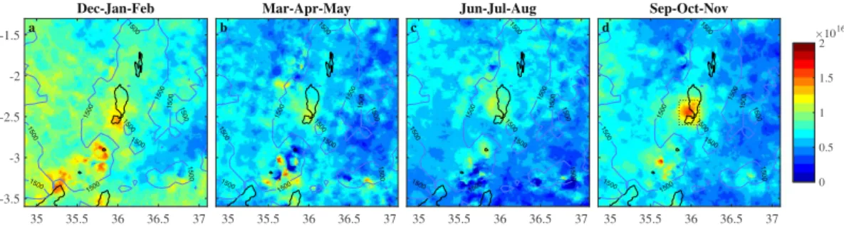
Seasonal NH3 column loadings averaged over Lake Natron and the immediate surroundings are shown in
Fig. 2 for IASI onboard Metop A and in Fig. S1 in the Supplementary Information for IASI onboard Metop B. Both the hotspot and the background area exhibit a strong seasonal cycle. The largest NH3 column loadings and
sharpest spatial gradients are observed over the hotspot during September to November. The NH3 measured in
these months evidently determines the location of the hotspot on an annual basis. However, a local NH3
maxi-mum is seen close to the lake during all seasons. The hotspot is slightly displaced to the south-east and diluted during the months December to February. The NH3 column loadings in the valley floor, and near Lake Victoria
are also highest in this season. The period March to August has the lowest column loadings both in the surround-ing area and over Lake Natron.
Figure 2. Seasonal NH3 column loading averages (molec/cm2) from IASI measurements onboard Metop A
for the period 2008–2017. The corresponding averages for IASI on Metop B are provided in Supplementary Information (Fig. S1). The hotspot area, indicated with a rectangle in panel (d) is used for timeseries analysis (Figs 4 and 5). The entire area shown was used to calculate the background NH3 column loadings in those
figures. a. 28.08.2017 b. 15.05.2013 c. 05.09.2010 d. 2013-2017 0 0.2 0.4 0.6 0.8 1
Figure 3. Variations in water extent illustrated and derived from MODIS imagery (MODIS corrected
reflectance imagery from NASA Worldview). Panel (a) shows the lake almost completely dry, panel (b) shows the lake at its maximum extent (see also Figs 5 and 6 of ref.16). The dates of these two extremes were found using the MODIS water product from the period 2013–2017. The frequency of detected water over each ~250 × 250 m2 area, as derived from the MODIS water product, is shown in panel (d). The 0.01 (almost always
dry) and 0.55 (flooded more than half of the time) frequency lake contours are indicated on the other panels with white dotted and solid lines, respectively. Panel (c) shows the situation on 5 September 2010, a day for which IASI measured large localized increased NH3 column loadings. The 2008–2017 NH3 averaged column
loadings are shown as coloured contours in panel (c) and visualize the location of the NH3 hotspot (the contours
Before continuing investigations of the hotspot, we discuss the observed seasonality of the background area (the entire area shown in Fig. 2). Monthly average NH3 column loadings over the background are shown in Fig. 4
(dotted red line). The background column loadings in January-February are almost double those in the other months. Meteorological variables provide clues as to the origin of this seasonality. Temperatures do not vary significantly throughout the year at Lake Natron. However, the lake has two wet seasons (see Fig. 4): a short one in November and December, and a longer one from February to May. A long dry season from May to October separates the two wetter periods. Biomass burning is an important emitter of atmospheric NH335, especially in
Africa, but the seasonality of the wet seasons immediately excludes fires as the origin of the background NH3.
The majority of the fires in the area take place in the Serengeti National Park (~100 km west of Lake Natron), in the middle of the dry season, between June and August (as shown in Fig. S2 in the Supplementary Information). Note also that the number of fires in the immediate vicinity of the lake is extremely low. Most of the observed background NH3 likely originates from agriculture as the observed NH3 average correlates spatially with livestock
numbers36. In particular, the largest background values of NH
3 are observed near Lake Victoria where livestock
densities are highest (Fig. 1). The seasonality of these emissions relates to the fact that NH3 from animal excreta
is only volatilized after chemical breakdown (hydrolysis) of urea, which requires sufficient amounts of water37. This precipitation effect has also been noted in other dry savannas in Africa38. More generally, rainfall stimulates organic matter mineralization in arid areas39. On the other hand, heavy rain transports dissolved NH
3 further
down in the surface40, which could explain why the largest NH
3 emissions occur between the two wet seasons,
when the soil is presumably at intermediate moisture levels.
Returning to the hotspot, the monthly timeseries in Fig. 4 (solid red line) confirms that the largest average column loadings occur from September to November, in addition to the (background) maximum in February. The normalized lake surface area shown in Fig. 4 (blue line) show that these maxima coincide with the end of the dry season in October-November, when the lake area is at its smallest, and between the two wet seasons, with a local minimum in surface area. To explore the link further between NH3 column loadings and lake surface area,
it is useful to look at shorter time scales. Daily NH3 column loadings over the hotspot area are shown in Fig. 5
for the entire period 2008–2017. Symbols are filled when the individual (daily) measured column loading over Lake Natron is the highest of the entire background area. Average background column loadings are indicated with black solid lines. For dates after 2013, the MODIS surface water extent is also shown. Note the large inter-annual variability of both NH3 and water extent. In certain years, strong emissions occur throughout the year
(e.g. in 2011, 2014 and 2017). In other years, atmospheric NH3 emissions are episodic and separated at times by
long quiescent periods. Such episodes took place e.g. in August–October 2010, September–November 2013 and August–November 2016. Shorter flares of the order of a week occur during October–November in most years. The variations in NH3 relate closely to the water extent, as seen for example for the prominent NH3 episodes in
2013 and 2016 that coincide with receding water levels. Prior to these episodes there was a long period of high water and NH3 column loadings that rarely exceeded background levels. On the other hand, throughout 2014
and 2017 large column loadings were observed and with a water fraction below 0.8, the lake never reached its maximum extent in those years. From this analysis we conclude that the largest NH3 emissions occur with the
drying of Lake Natron’s mudflats.
Before exploring possible mechanisms to explain these emissions, it is important to exclude other possible processes that could explain the observed seasonality. Agricultural emissions from the surrounding areas, and pastoralism in the Natron basin may contribute to the peak in the wet season. However, herding is too disperse around Lake Natron to explain the intensity or the location of the hotspot directly over the lake’s mudflat, where livestock never comes. The different seasonality and limited spatial extent of the hotspot indicate that another
Figure 4. 2008–2017 monthly averages of the rainfall amount (histogram, derived from ECMWF’s ERA5
data on the model output at 35.91°E, 2.49°S), the normalized lake area (blue, derived from the MODIS water product), the IASI NH3 column loadings (molec/cm2) over the hotspot area (solid red line) and over the
mechanism drives the majority of the hotspot’s emissions. A potential explanation of the observed seasonality could be found in the existence of possible seasonal biases in the NH3 measurements, related in particular to
variations in thermal contrast and the planetary boundary layer (PBL) height. Thermal contrast (which is the difference between the temperature of the surface and air) is known to largely affect measurement sensitivity in the infrared spectral domain41. However, the Lake Natron area provides almost ideal conditions for accurate and sensitive satellite measurements of NH3 with a stable mean thermal contrast of ~10 K for all months at the
overpass time of IASI (9.30 in the morning). The PBL height affects greatly the vertical distribution of NH3 and as
the NH3 retrieval algorithm assumes a fixed constant vertical profile, large seasonal differences in the PBL height
Jan Feb Mar Apr May Jun Jul Aug Sep Oct Nov Dec 2008 0 1 2 3 NH 3 (molec/cm 2) 1016 0 0.2 0.4 0.6 0.8 1
Jan Feb Mar Apr May Jun Jul Aug Sep Oct Nov Dec 2009 0 1 2 3 NH 3 (molec/cm 2) 1016 0 0.2 0.4 0.6 0.8 1
Jan Feb Mar Apr May Jun Jul Aug Sep Oct Nov Dec 2010 0 1 2 3 NH 3 (molec/cm 2) 1016 0 0.2 0.4 0.6 0.8 1
Jan Feb Mar Apr May Jun Jul Aug Sep Oct Nov Dec 2011 0 1 2 3 NH 3 (molec/c m 2) 1016 0 0.2 0.4 0.6 0.8 1
Jan Feb Mar Apr May Jun Jul Aug Sep Oct Nov Dec 2012 0 1 2 3 NH 3 (molec/c m 2) 1016 0 0.2 0.4 0.6 0.8 1
Jan Feb Mar Apr May Jun Jul Aug Sep Oct Nov Dec 2013 0 1 2 3 1016 0 0.2 0.4 0.6 0.8 1
Lake area (normalized
)
Jan Feb Mar Apr May Jun Jul Aug Sep Oct Nov Dec 2014 0 1 2 3 1016 0 0.2 0.4 0.6 0.8 1
Lake area (normalized)
Jan Feb Mar Apr May Jun Jul Aug Sep Oct Nov Dec 2015 0 1 2 3 1016 0 0.2 0.4 0.6 0.8 1
Lake area (normalized)
Jan Feb Mar Apr May Jun Jul Aug Sep Oct Nov Dec 2016 0 1 2 3 1016 0 0.2 0.4 0.6 0.8 1
Lake area (normalized)
Jan Feb Mar Apr May Jun Jul Aug Sep Oct Nov Dec 2017 0 1 2 3 1016 0 0.2 0.4 0.6 0.8 1
Lake area (normalized)
Figure 5. Timeseries of atmospheric NH3 (molec/cm2) over Lake Natron. Individual NH3 column loadings
observed over the hotspot area are plotted with diamond symbols. Solid diamonds indicate that the observed NH3 column loading over the hotspot area is a local maximum, that is higher than the other measured column
loadings of the larger background area. Mean background column loadings, calculated over an area that extends the hotspot area by 1° on all sides (see Fig. 2), are represented with solid black lines. The MODIS water extent, expressed as fraction of the maximum is shown in blue for the period 2013–2017. To simplify analysis, both the background column loadings and the water fraction were smoothed in time.
could result in a seasonal biases in the retrieved columns (ref.42 reports biases of around 50% between a PBL of 100 m versus that of a 2 km one). An analyses of ERA543 PBL heights at Lake Natron however, shows very little seasonal variation (at the IASI overpass time the yearly average is 984 m with a standard deviation of 253 m, a minimum monthly average of 866 m in June and a maximum of 1119 m in October). Another aspect that should be considered is that of wind dispersion. NH3 total column loadings that satellites measure only correlate well
with emissions if the NH3 atmospheric lifetime is constant. For instance, strong winds in one season could reduce
the build-up of NH3 directly above the lake. ERA5 surface wind fields indicate a marked seasonality in wind speed
strength, with the strongest winds (2.2–2.8 m/s) in the period May to October, and weaker winds (1.7–2 m/s) in the other months. If the lack of dispersion would explain the seasonality, a NH3 maximum could not be seen in
September. Wind directions appear randomly distributed, with no apparent seasonality. Finally, we consider and exclude the existence of measurement artefacts, which is the subject of next section.
spectroscopic evidence
Since no obvious NH3 source was initially identified at Lake Natron, it was early on suspected that the hotspot was
due to a retrieval artefact rather than an actual NH3 enhancement. Retrieval artefacts may occur when spectra
exhibit unusual features in the spectral region of interest. These ‘unusual features’ are due to atmospheric constit-uents that are difficult to model (e.g. aerosols44) or specific surface types (e.g. sand, snow and ice45).
Surface effects manifest themselves especially in the ‘atmospheric window’ between 800–1200 cm−1. This
spec-tral range is largely transparent for infrared radiation, so that the largest portion of the radiation observed on top of the atmosphere originates from the surface. Hence, spectral variations in surface emissivity, expressing the deviation of the surface from the theoretical black body, impact the observed spectrum46. The peculiar visible appearance of Lake Natron with its salt encrusted (mud)flats, and the fact that the NH3 retrieval relies fully on
the atmospheric window, therefore calls for a careful investigation of possible surface retrieval artefacts. An ear-lier analysis of outear-liers in the principle component reconstruction of IASI spectra, revealed that soda lakes can indeed exhibit very large and sharp emissivity features47,48. The most extreme example for Lake Natron, for the entire period of IASI observations, is shown in Fig. 6. It was observed on 15 December 2007 right above the main mudflats. Although this example does not reflect common observations over Lake Natron, it helps identifying the relevant features, and illustrates the worst case behaviour.
A large feature between 1070 and 1240 cm−1 is apparent as well as a smaller one between 830 and 890 cm−1.
The larger one may relate to a mineral with a SO − 4
2 functional group, which has a strong vibrational mode in this range49,50. There is a good match with the emissivity spectrum of gypsum, but this mineral is highly unlikely to be seen over Lake Natron given its alkaline Calcium-deprived soil51. A plausible candidate is kogarkoite [Na
3(SO4)
F], previously identified at Lake Natron17,52–54. Its transmittance spectrum55 is compatible with the observed
750 800 850 900 950 1000 1050 1100 1150 1200 1250 Wavenumber (cm-1) 260 265 270 275 280 285 290 295 300 305 Brightness Temperature (K) HCO3- CO3 2- SO4 2-a b c -0.2 0 0.2 0.4 0.6 d -0.5 0 0.5 1
Figure 6. IASI spectrum observed over Lake Natron on 15 December 2007, evening overpass is shown in
panel (a). Only the part of the spectra most relevant for the NH3 retrieval is depicted. The location of the IASI
footprint is shown in panel (b) on the right superimposed over visible MODIS Terra imagery from the day after (the MODIS image of the 15th is more blurry but similar). Panel (a) also shows the position of the three large identified emissivity features, as indicated by thick black lines and their suspected associated functional groups. Mean brightness temperature differences between two baseline channels (black crosses) and two affected channels (red crosses) quantize the emissivity features. Selected channels are in increasing order of wavenumber: 833.5, 861.5, 874.5, 899.75, 1079.25, 1153.75, 1157.75 and 1231.5 cm−1. Since the two features near
850 cm−1 partially overlap, they were characterized by a single brightness temperature difference. The insets c
and d show the 10-year oversampled average of both brightness temperature differences calculated using all 2008–2017 IASI observations (morning overpass). MODIS imagery is the corrected reflectance imagery from NASA Worldview.
feature. Other candidate sulfate minerals include thenardite [Na2SO4], burkeite [Na2CO3 · 2Na2SO4] and
mirabi-lite [Na2SO4 · 10H2O], but these have to our knowledge not been identified at Lake Natron.
The dip in the spectrum between 830 and 890 cm−1 is composed of two features, one centred around 853 cm−1
and a broader one between 840 and 890 cm−1. This is not apparent from this example spectra, but a comparison
with other spectra reveals that both features occur with varying intensity. The feature around 853 cm−1 may relate
to vibrations of the HCO−
3 group as it matches nicely with published reflectance spectra of trona (Na2CO3 · NaHCO3 · 2H2O)56,57. The broader feature is likely due to the CO23− group49. Natron (Na2CO3 · 10H2O)
and thermonatrite (Na2CO3 · H2O) have spectra that are compatible (see56 and the RELAB spectral database).
However, natron can be excluded as it does not precipitate at Lake Natron, contrary to what its name would sug-gest17. Other evaporites that are found at Lake Natron are halite (NaCl) and villiaumite (NaF). Halite does not exhibit a strong spectral variation in the atmospheric window. A reference spectrum of villiaumite was unfortu-nately not found. Therefore, with the available information, we assign the observed emissivity features to trona, thermonatrite and kogarkoite.
To assess where, how often and with what intensity emissivity features occur, Brightness Temperature Differences (BTDs) can be used. These are differences between affected and unaffected IASI channels and quan-titatively express the magnitude of spectral features. A BTD was constructed for both features (the double feature between 830 and 890 cm−1 was characterized by a single BTD). Details are shown in Fig. 6. The resulting 2008–
2017 averages are shown as insets. The largest values are observed in about the same location as the NH3 hotspot,
where the lake is exposed most. However, unlike the NH3 enhancements, they are also observed over the entire
lake surface. The seasonality (see Fig. S3 in the Supplementary Information) reveals that the emissivity features are observed with varying intensity, but throughout the year. Especially the feature associated with the SO − 4 2 group has a clear maximum in December to February, when the lake undergoes rapid cycles of rewetting and evaporation (see Fig. 5). This timing suggests that the observed surface emissivity effects are most pronounced after fresh crystallization. This may also explain why the features are best seen on IASI’s evening overpass (the spectrum of Fig. 6 was observed in the evening). Importantly, note that the seasonality does not match the observed NH3 cycle. This largely excludes the possibility of retrieval artefacts in the NH3 data related to these
significant emissivity features. As a side remark, the above analysis indicates that IASI and other hyperspectral polar orbiters could be exploited for the imaging of surface minerals, something that has been traditionally pre-served for imaging instruments58.
For retrievals that rely on a physical reconstruction of the spectrum, (smaller) retrieval artefacts can be exposed by analysing the difference between the observed and calculated spectrum (i.e. the residual of the fit). However, such residuals are not available as part of the IASI NH3 dataset used in this study, as the retrieval algorithm does
not attempt to reconstruct the observed spectra. Therefore, to exclude the existence of smaller retrieval artefacts and more importantly to provide explicit spectroscopic evidence of the presence of NH3, we performed spectral
fits on selected spectra observed over Lake Natron. Figure 7 shows a fit (in red) of a spectrum observed (in blue) on 5 September 2010 over the hotspot area. NH3, surface temperature, O3 and H2O atmospheric concentrations
were adjusted to match the observed spectrum via an optimal estimation approach41. The retrieval range was lim-ited to 878–1144 cm−1 to avoid the sharpest of the emissivity features. Observe that the spectrum is reconstructed
adequately over this entire spectral range. From the retrieved parameters, a second spectrum can be simulated
Figure 7. (Panel (a)) Example of an IASI spectrum (blue) where a large NH3 column loading is measured
and the fitted spectrum (red). Panel (b) shows the residual including the NH3 contribution (blue) and the
NH3 contribution itself (green), see details in the text. MODIS imagery recorded on the same day is shown
in panel (c), superimposed are the IASI NH3 observations of that day. These are coloured according to the
colorbar of Fig. 1 (from 0 to 2 · 1016 molec/cm2). The ellipses approximate the actual footprint on ground of the
measurements. The spectrum on the left corresponds to the red ellipse observed directly over Lake Natron. MODIS imagery is the corrected reflectance imagery from NASA Worldview.
that represents what would be observed if NH3 was not present in the atmosphere. The difference between the two
simulations, with and without NH3 in the simulation, allows visualization of the NH3 contribution in the fitted
spectrum (here shown in green). The difference between the observed spectrum and the simulation without NH3,
shown here in blue, demonstrates that the NH3 signature exceeds the instrumental noise and other features not
accounted for in the retrieval. This constitutes the first piece of explicit evidence for the presence of NH3.
The fit, presented here, was obtained from three separate retrievals conducted in different spectral bands (878–969 cm−1, 970–1075 cm−1 and 1074–1144 cm−1). This allows obtaining several independent estimates of the
NH3 column loading from a single spectrum. Surface concentrations of 17, 16 and 13 ppb were obtained for this
particular spectrum (IASI measures column loadings, we converted them into estimated surface concentrations by assuming an average vertical profile59). Because all three values agree well, the possibility of a retrieval artefact can be ruled out almost entirely. The fact that these results also agree with the 15 ppb value retrieved by the main IASI NH3 algorithm provides further confidence on the robustness of the fits, and on the concentrations retrieved
by the main algorithm.
Even though the presence of NH3 over Lake Natron is confirmed on the 5 September 2010, it is possible that
the observed NH3 on that day was emitted elsewhere. For this reason, the analysis presented above was repeated
on a series of spectra from observations of IASI on Metop A and Metop B. Selected examples are shown in Figs S4 to S7 of the Supplementary Information. To minimize the possibility of observing transported NH3, cases were
selected where a sharp local NH3 enhancement was observed over the hotspot area. Unsurprisingly, all these
chosen examples ended up being from September and October. Each of these examples reveal an unambiguous NH3 signature with consistent retrieval results across the different bands, providing further confidence that the
NH3 hotspot is genuine.
sources and mechanisms
Due to the absence of outflow, endorheic lakes accumulate in addition to salts also nutrients and organic matter, which maintain via internal cycling the active biological production60,61. Decomposition and associated ammoni-fication of nutrient rich organic matter62,63 appears to be the principal source of NH
3 in African soda lakes22,28,64,65.
This includes breakdown of plankton66, droppings of flamingos and other waterbirds65,67,68 and miscellaneous organic material carried in via the rivers or hot springs (plant residues, agricultural run-off and waste of mammals and humans69). Wetland soil sediments in particular act as a major reservoir of nitrogen and release significant amounts of NH362,70, and this is probably not different at Lake Natron whose mudflats are composed of layers of
silt and organic material71. Flamingos play an important role in the nitrogen cycle of soda lakes, via their feeding and excreting, but also through sediment bioturbation65,72,73. However, their precise contribution to the NH
3
emissions at Lake Natron can only be elucidated with the help of dedicated longterm monitoring data. In terms of input of reactive nitrogen, we expect the feeding and excretion processes of flamingos to average out. The domi-nant net input to this lake is likely the influx via rivers.
Water measurements in African soda lakes typically yield high concentrations of dissolved organic nitrogen. Reported inorganic nitrogen concentrations are variable61,64,66. At Lake Natron, 8 μg/L NO−
3 and 58 μg/L NH3/NH+4 were reported recently22. One probable cause for low NH3 concentrations is that the conditions in soda
lakes favour volatilization64,74. The main argument is that increasing alkalinity and temperature shift the +
NH4 + OH− NH
3 + H2O equilibrium in a soil or water solution towards the right75. As an example, neutral
solutions at room temperature contain as much as 99.5% NH+
4, while for typical Natron conditions of a pH of 10 and a temperature of 35 °C, 92% of ammoniacal N in solution is present as NH376 (but see ref.77). NH3 losses are
further promoted by elevated temperatures that favour NH3 gas removal at the surface-air interface and strong
surface winds over the rift valley floor, which dominate in the dry season71.
The cited sources of NH3 and these favourable conditions for volatilization alone do not explain the hotspot at
Lake Natron, as these elements are also found in other African soda lakes that do not exhibit elevated atmospheric NH3 column loadings. A good example of this is Lake Nakuru (see Fig. 1), which is also a soda lake (pH above
1066,78), with a much larger anthropogenic input of nitrogen79, and with high flamingo populations24. The peri-odic flooding and drying of vast mudflats is however more specific to Lake Natron (other examples are discussed below). Also the timeseries analysis presented before, suggests that the mechanism of massive NH3 volatilization
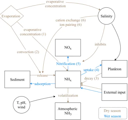
should specifically be linked to its drying process. Here we provide six additional processes that may contribute: 1. Evaporative concentration. NH3 concentration, is by definition reversely proportional to the amount of
liquid. As the soil–water surface dries up, the available NH3 concentrates, which increases the
surface-at-mosphere concentration gradient, resulting in increased volatilization to maintain the equilibrium40,80. 2. Convection. Upon soil evaporation, dissolved NH3 can be transported to the surface along with the upward
movement of water75.
3. Decay of plankton. Reduced water availability and increased salinity eventually leads to die-off of plankton and subsequent breakdown and ammonification of the biomass.
4. Assimilation. Reduced biological activity also leads to a decreased uptake of NH3.
5. Nitrification. Ammonia oxidizing bacteria can limit nitrogen losses in soda lakes, however this mecha-nism is no longer available in concentrated brines as nitrification is inhibited beyond a certain salinity threshold74,81.
6. Cation exchange and ion pairing. The cation exchange complex determines how much NH+ 4 can be reversible adsorbed on soil colloids. Silts and organic material in principle favour a high cation exchange coefficient and therefore help retaining NH+
4 in the soil82. However, high concentrations of Na+ can outcompete and displace NH+
4 in the available soil exchange sites. In addition, ion pair formation with anions in the surface water may stimulate diffusion of NH+ out of the sediment81,83,84.
A simplified conceptual model of the above processes is presented in Fig. 8. The positive correlation between salinity and NH3 concentration, expected from several of these, has been reported by in-situ measurements in
both saline81 and soda lakes65,85.
We consider briefly the question whether elevated NH3 column loadings may be observed over other nearby
Eastern Rift Valley lakes. At least four soda lakes are shallow and have regularly flooded/exposed saline mudflats (see Fig. 1): Lake Eyasi, Lake Manyara, Lake Magadi and Lake Logipi. These are also important flamingo lakes86. Lake Magadi neighbours Lake Natron and resembles it in many ways. However, its mudflats are much smaller in surface area which may explain why no convincing enhancements are observed. A small NH3 hotspot is detected
at Lake Logipi61, over mudflats just south of the permanent water body. The location and timing are consistent with the patterns observed at Lake Natron, but relatively low column loadings, larger year-to-year variability and the absence of a clear seasonal cycle make it even more challenging to analyse. Enhancements over Lake Logipi are seen in the years 2008 to 2012 (2012 is the record year). Surprisingly, in subsequent years 2013–2016 the hot-spot disappeared, but re-emerged in 2017. A small hothot-spot is seen near the centre of Lake Manyara, but a larger background makes it difficult to conclude anything. No NH3 hotspot is seen at Lake Eyasi.
It is our hope that the results presented in this study will spur on future studies driven by in situ measurements of nutrient concentrations, nitrogen dynamics and observations of environmental factors at Lake Natron and other similar lakes. Examples of the latter would be data on biomass growth and die-off, and on the distribution of the highly nomadic lesser flamingos. Especially temporal data that can be linked with the timeseries pre-sented here would be most welcome (e.g. the few bird censuses that are available date before 200787–90, or are for other lakes72,91). Such ground-truth data will allow determining the dominant mechanisms at play and ultimately improve our understanding of the nitrogen cycle in soda lakes.
Data Availability
The IASI data used in this study has been archived in the PANGAEA repository (10.1594/PANGAEA.895632); Other IASI NH3 data is available from the Aeris data infrastructure (http://iasi.aeris-data.fr).
References
1. Fowler, D. et al. The global nitrogen cycle in the twenty-first century. Phil. Trans. R. Soc. B 368, 20130164, https://doi.org/10.1098/ rstb.2013.0164 (2013).
2. Erisman, J. W., Sutton, M. A., Galloway, J., Klimont, Z. & Winiwarter, W. How a century of ammonia synthesis changed the world.
Nature Geosci. 1, 636–639, https://doi.org/10.1038/ngeo325 (2008).
3. Galloway, J. et al. Nitrogen cycles: past, present and future. Biogeochemistry 70, 153–226, https://doi.org/10.1007/s10533-004-0370-0 (2004).
4. Lamarque, J.-F. et al. Global and regional evolution of short-lived radiatively-active gases and aerosols in the representative concentration pathways. Climatic Change 109, 191, https://doi.org/10.1007/s10584-011-0155-0 (2011).
Figure 8. A simplified conceptual model of the different processes that link evaporation and soil drying to NH3
5. Erisman, J. W. et al. Consequences of human modification of the global nitrogen cycle. Philos. Trans. R. Soc. London, Ser. B 368, 20130116–20130116, https://doi.org/10.1098/rstb.2013.0116 (2013).
6. Warneck, P. Chemistry of the Natural Atmosphere, chap. 9. Nitrogen compounds in the troposphere, 511–586 (Elsevier, 2000). 7. Behera, S. N., Sharma, M., Aneja, V. P. & Balasubramanian, R. Ammonia in the atmosphere: a review on emission sources,
atmospheric chemistry and deposition on terrestrial bodies. Environ. Sci. Pollut. Res. Int. 20, 8092–8131, https://doi.org/10.1007/ s11356-013-2051-9 (2013).
8. Clarisse, L., Clerbaux, C., Dentener, F., Hurtmans, D. & Coheur, P.-F. Global ammonia distribution derived from infrared satellite observations. Nature Geosci. 2, 479–483, https://doi.org/10.1038/ngeo551 (2009).
9. Warner, J. X. et al. Increased atmospheric ammonia over the world’s major agricultural areas detected from space. Geophys. Res. Lett.
44, 2875–2884, https://doi.org/10.1002/2016gl072305 (2017).
10. Shephard, M. W. et al. TES ammonia retrieval strategy and global observations of the spatial and seasonal variability of ammonia.
Atmos. Chem. Phys. 11, 10743–10763, https://doi.org/10.5194/acp-11-10743-2011 (2011).
11. Shephard, M. W. & Cady-Pereira, K. E. Cross-track Infrared Sounder (CrIS) satellite observations of tropospheric ammonia. Atmos.
Meas. Tech. 8, 1323–1336, https://doi.org/10.5194/amt-8-1323-2015 (2015).
12. Van Damme, M. et al. Global distributions, time series and error characterization of atmospheric ammonia (NH3) from IASI satellite
observations. Atmos. Chem. Phys. 14, 2905–2922, https://doi.org/10.5194/acp-14-2905-2014 (2014).
13. Van Damme, M. et al. Industrial and agricultural ammonia point sources exposed. Nature 564, 99–103, https://doi.org/10.1038/ s41586-018-0747-1 (2018).
14. Van Damme, M. et al. Version 2 of the IASI NH3 neural network retrieval algorithm: near-real-time and reanalysed datasets. Atmos. Meas. Tech. 10, 4905–4914, https://doi.org/10.5194/amt-10-4905-2017 (2017).
15. Vincens, A. & Casanova, J. Modern background of Natron-Magadi basin (Tanzania-Kenya): physiography, climate, hydrology and vegetation. Sci. Géol. Bull. 40, 9–21 (1987).
16. Tebbs, E., Remedios, J., Avery, S. & Harper, D. Remote sensing the hydrological variability of Tanzania’s Lake Natron, a vital Lesser Flamingo breeding site under threat. Ecohydrol. Hydrobiol. 13, 148–158, https://doi.org/10.1016/j.ecohyd.2013.02.002 (2013). 17. Warren, J. K. Evaporites. A geological compendium. Second edition, 344–353, https://doi.org/10.1007/978-3-319-13512-0 (Springer,
2016).
18. Schagerl, M. & Renaut, R. W. Dipping into the Soda Lakes of East Africa. In Schagerl, M. (ed.) Soda Lakes of East Africa, chap. 1, 3–24, https://doi.org/10.1007/978-3-319-28622-8_1 (Springer International Publishing, 2016).
19. Grant, W. Alkaline environments and biodiversity. In Gerday, C. & Glansdorff, N. (eds) Extremophilies, Encyclopedia of Life Support Systems (EOLSS) (Eolss Publishers, Oxford, UK, 2006).
20. Oduor, S. O. & Schagerl, M. Phytoplankton primary productivity characteristics in response to photosynthetically active radiation in three Kenyan Rift Valley saline alkaline lakes. J. Plankton Res. 29, 1041–1050, https://doi.org/10.1093/plankt/fbm078 (2007). 21. Tebbs, E., Remedios, J., Avery, S., Rowland, C. & Harper, D. Regional assessment of lake ecological states using Landsat: A
classification scheme for alkaline–saline, flamingo lakes in the East African Rift Valley. Int. J. Appl. Earth Obs. Geoinf. 40, 100–108,
https://doi.org/10.1016/j.jag.2015.03.010 (2015).
22. Nonga, H. et al. Cyanobacteria and cyanobacterial toxins in the alkaline-saline Lakes Natron and Momela, Tanzania. In Proceedings
of the 34th scientific conference of the Tanzania Veterinary Association, vol. 32, 108–116 (Arusha, Tanzania, 2017).
23. Brown, L. H. & Root, A. The breeding behaviour of the Lesser Flamingo Phoeniconaias Minor. Ibis 113, 147–172, https://doi. org/10.1111/j.1474-919x.1971.tb05141.x (1971).
24. Krienitz, L., Mähnert, B. & Schagerl, M. Lesser Flamingo as a central element of the East African avifauna. In Schagerl, M. (ed.) Soda
Lakes of East Africa, 259–284, https://doi.org/10.1007/978-3-319-28622-8_10 (Springer International Publishing, 2016). 25. Ford, A. G. P. et al. High levels of interspecific gene flow in an endemic cichlid fish adaptive radiation from an extreme lake
environment. Mol. Ecol. 24, 3421–3440, https://doi.org/10.1111/mec.13247 (2015).
26. Kavembe, G. D., Meyer, A. & Wood, C. M. Fish populations in East African saline lakes. In Schagerl, M. (ed.) Soda Lakes of East
Africa, 227–257, https://doi.org/10.1007/978-3-319-28622-8_9 (Springer International Publishing, 2016).
27. Norconsult. Environmental and social impact assessment for the development of a soda ash facility at Lake Natron, Tanzania (2007). 28. Bettinetti, R. et al. A preliminary evaluation of the DDT contamination of sediments in Lakes Natron and Bogoria (Eastern Rift
Valley, Africa). AMBIO 40, 341–350, https://doi.org/10.1007/s13280-011-0142-8 (2011).
29. Baker, M. Lake Natron, Flamingos and the Proposed Soda Ash Factory, Tanzania Natural Resource Forum (2011).
30. Kadigi, R. M. J., Mwathe, K., Dutton, A., Kashaigili, J. & Kilima, F. Soda ash mining in Lake Natron: A reap or ruin for Tanzania?
Journal of Environmental Conservation Research 2, 37, https://doi.org/10.12966/jecr.05.01.2014 (2014). 31. TheEastAfrican. Tanzania shelves Lake Natron soda ash project (2018).
32. Snyder, K. A. & Sulle, E. B. Tourism in Maasai communities: a chance to improve livelihoods? J. Sust. Tour. 19, 935–951, https://doi. org/10.1080/09669582.2011.579617 (2011).
33. NASA Earth Observatory. Lake Natron, Tanzania photograph taken from the International Space Station on 11 November 2002 (2002).
34. Policelli, F. et al. The NASA global flood mapping system. In Lakshmi, V. (ed.) Remote Sensing of Hydrological Extremes, 47–63,
https://doi.org/10.1007/978-3-319-43744-6_3 (Springer International Publishing, Cham, 2017).
35. Whitburn, S. et al. Ammonia emissions in tropical biomass burning regions: Comparison between satellite-derived emissions and bottom-up fire inventories. Atmos. Environ. 121, 42–54, https://doi.org/10.1016/j.atmosenv.2015.03.015 (2015).
36. Robinson, T. P. et al. Mapping the global distribution of livestock. PLoS One 9, e96084, https://doi.org/10.1371/journal.pone.0096084
(2014).
37. Reynolds, C. M. & Wolf, D. C. Effect of soil moisture and air relative humidity on ammonia volatilization from surface-applied urea.
Soil Sci. 143, 144–152, https://doi.org/10.1097/00010694-198702000-00010 (1987).
38. Adon, M. et al. Dry deposition of nitrogen compounds (NO2, HNO3, NH3), sulfur dioxide and ozone in west and central African
ecosystems using the inferential method. Atmos. Chem. Phys. 13, 11351–11374, https://doi.org/10.5194/acp-13-11351-2013 (2013). 39. Schlesinger, W. H. & Peterjohn, W. T. Processes controlling ammonia volatilization from Chihuahuan desert soils. Soil Biol. Biochem.
23, 637–642, https://doi.org/10.1016/0038-0717(91)90076-v (1991).
40. Francis, D. D., Vigil, M. F., Mosier, A. R., Schepers, J. S. & Raun, W. R. Gaseous losses of nitrogen other than through denitrification. In Nitrogen in Agricultural Systems, 255–279, https://doi.org/10.2134/agronmonogr49.c8 (American Society of Agronomy, Crop Science Society of America, Soil Science Society of America, 2008).
41. Clarisse, L. et al. Satellite monitoring of ammonia: A case study of the San Joaquin Valley. J. Geophys. Res. 115, D13302, https://doi. org/10.1029/2009JD013291 (2010).
42. Whitburn, S. et al. A flexible and robust neural network IASI-NH3 retrieval algorithm. J. Geophys. Res. 121, 6581–6599, https://doi.
org/10.1002/2016jd024828 (2016).
43. Copernicus Climate Change Service (C3S): ERA5: Fifth generation of ECMWF atmospheric reanalyses of the global climate. Copernicus Climate Change Service Climate Data Store (CDS) (2018).
44. Maddy, E. S. et al. On the effect of dust aerosols on AIRS and IASI operational level 2 products. Geophys. Res. Lett. 39, L10809,
https://doi.org/10.1029/2012GL052070 (2012).
45. Bauduin, S. et al. Retrieval of near-surface sulfur dioxide (SO2) concentrations at a global scale using IASI satellite observations. Atmos. Meas. Tech. 9, 721–740, https://doi.org/10.5194/amt-9-721-2016 (2016).
46. Eastes, J. W. Spectral and physical properties of some desert soils: Implications for remote spectroscopic terrain analysis in arid regions. Appl. Spectrosc. 46, 640–644 (1992).
47. Atkinson, N. C., Hilton, F. I., Illingworth, S. M., Eyre, J. R. & Hultberg, T. Potential for the use of reconstructed IASI radiances in the detection of atmospheric trace gases. Atmos. Meas. Tech. 3, 991–1003, https://doi.org/10.5194/amt-3-991-2010 (2010).
48. Chefdeville, S. Analyse de trois années d’ outliers dans les mesures de l’instrument IASI: détection et étude d’évènements extrêmes, Internship report (Université libre de Bruxelles (ULB), 2010).
49. Socrates, G. Infrared and Raman Characteristic Group Frequencies. Tables and Charts. Third Edition (John Wiley & Sons, 2001). 50. Lane, M. D. Mid-infrared emission spectroscopy of sulfate and sulfate-bearing minerals. Am. Mineral. 92, 1–18, https://doi.
org/10.2138/am.2007.2170 (2007).
51. Eugster, H. P. Lake Magadi, Kenya: a model for rift valley hydrochemistry and sedimentation? Geol. Soc. Spec. Publ. 25, 177–189,
https://doi.org/10.1144/gsl.sp.1986.025.01.15 (1986).
52. Darragi, F., Gueddari, M. & Fritz, B. Mise en evidence d’un fluoro-sulfate de sodium, la kogarkoite, dans les croutes salines du Lac Natron en Tanzanie (Presence of Kogarkoite (Na3SO4F) in the salt paragenesis of Lake Natron in Tanzania). Comptes-Rendus des Seances de l’Academie des Sciences Serie 2 297, 141–144 (1983).
53. Nielsen, J. M. East African magadi (trona): fluoride concentration and mineralogical composition. J. Afr. Earth. Sci. 29, 423–428,
https://doi.org/10.1016/s0899-5362(99)00107-4 (1999).
54. Mitchell, R. H. Mineralogy of stalactites formed by subaerial weathering of natrocarbonatite hornitos at Oldoinyo Lengai, Tanzania.
Mineral. Mag. 70, 437–444, https://doi.org/10.1180/0026461067040344 (2006). 55. Chukanov, N. V. Infrared spectra of mineral species. Extended library (Springer, 2014).
56. Huang, C. K. & Kerr, P. F. Infrared study of the carbonate minerals. Am. Mineral. 45, 311–324 (1960).
57. Baldridge, A., Hook, S., Grove, C. & Rivera, G. The ASTER spectral library version 2.0. Remote Sens. Environ. 113, 711–715, https:// doi.org/10.1016/j.rse.2008.11.007 (2009).
58. Kodikara, G. R. et al. Hyperspectral remote sensing of evaporate minerals and associated sediments in Lake Magadi area, Kenya. Int.
J. Appl. Earth Obs. Geoinf. 14, 22–32, https://doi.org/10.1016/j.jag.2011.08.009 (2012).
59. Van Damme, M. et al. Towards validation of ammonia (NH3) measurements from the IASI satellite. Atmos. Meas. Tech. 8,
1575–1591, https://doi.org/10.5194/amt-8-1575-2015 (2015).
60. Duarte, C. M. et al. CO2 emissions from saline lakes: A global estimate of a surprisingly large flux. Journal of Geophysical Research: Biogeosciences 113, https://doi.org/10.1029/2007jg000637 (2008).
61. Castanier, S., Bernet-Rollande, M.-C., Maurin, A. & Perthuisot, J.-P. Effects of microbial activity on the hydrochemistry and sedimentology of Lake Logipi, Kenya. Hydrobiologia 267, 99–112, https://doi.org/10.1007/BF00018793 (1993).
62. White, J. R. & Reddy, K. R. Biogeochemical dynamics I: Nitrogen cycling in wetlands. In Maltby, E. & Barker, T. (eds) The Wetlands
Handbook, 213–227, https://doi.org/10.1002/9781444315813.ch9 (Wiley-Blackwell, 2009).
63. Herbert, R. Nitrogen cycling in coastal marine ecosystems. FEMS Microbiology Reviews 23, 563–590, https://doi. org/10.1111/j.1574-6976.1999.tb00414.x (1999).
64. Oduor, S. O. & Schagerl, M. Temporal trends of ion contents and nutrients in three Kenyan Rift Valley saline-alkaline lakes and their influence on phytoplankton biomass. In Shallow Lakes in a Changing World, 59–68, https://doi.org/10.1007/978-1-4020-6399-2_6
(Springer Netherlands, 2007).
65. Kihwele, E., Lugomela, C., Howell, K. & Nonga, H. Spatial and temporal variations in the abundance and diversity of phytoplankton in Lake Manyara, Tanzania. International Journal of Innovative Studies in Aquatic Biology and Fisheries 1 (2015).
66. Kulecho, A. & Muhandiki, V. Water quality trends and input loads to Lake Nakuru. In Proceedings of the 11th World Lakes
Conference, Nairobi, Kenya, 31 October to 4 November 2005, vol. II, 529–533 (2005).
67. Ganning, B., Wulff, F. & Ganning, B. The effects of bird droppings on chemical and biological dynamics in brackish water rockpools.
Oikos 20, 274, https://doi.org/10.2307/3543194 (1969).
68. Riddick, S. et al. The global distribution of ammonia emissions from seabird colonies. Atmos. Environ. 55, 319–327, https://doi. org/10.1016/j.atmosenv.2012.02.052 (2012).
69. Gichuki, N. N., Oyieke, H. A. & Terer, T. Status and root causes of biodiversity loss in the eastern Rift Valley lakes, Kenya. In
Proceedings of the 11th World Lakes Conference, Nairobi, Kenya, 31 October to 4 November 2005, vol. II, 511–517 (2005).
70. Jellison, R., Miller, L. G., Melack, J. M. & Dana, G. L. Meromixis in hypersaline Mono Lake, California. 2. Nitrogen fluxes. Limnol.
Oceanogr. 38, 1020–1039, https://doi.org/10.4319/lo.1993.38.5.1020 (1993).
71. Manega, P. C. & Bieda, S. Modern sediments of Lake Natron, Tanzania. Sci. Géol. Bull. 40, 83–95 (1987).
72. Kihwele, E. S., Lugomela, C. & Howell, K. M. Temporal changes in the Lesser Flamingos population (Phoenicopterus minor) in relation to phytoplankton abundance in Lake Manyara, Tanzania. Open Journal of Ecology 04, 145–161, https://doi.org/10.4236/ oje.2014.43016 (2014).
73. Batanero, G. L. et al. Flamingos and drought as drivers of nutrients and microbial dynamics in a saline lake. Scientific Reports 7,
https://doi.org/10.1038/s41598-017-12462-9 (2017).
74. Sorokin, D. Y. et al. Microbial diversity and biogeochemical cycling in soda lakes. Extremophiles 18, 791–809, https://doi. org/10.1007/s00792-014-0670-9 (2014).
75. Freney, J., Simpson, J. & Denmead, O. Volatilization of ammonia. In Freney, J. & Simpson, J. (eds) Gaseous Loss of Nitrogen from
Plant-Soil Systems, 1–32, https://doi.org/10.1007/978-94-017-1662-8_1 (Springer, 1983).
76. Cai, G.-X. Ammonia volatilization. In Zhu, Z.-l., Wen, Q.-x. & Freney, J. R. (eds) Nitrogen in Soils of China, 193–213, https://doi. org/10.1007/978-94-011-5636-3_9 (Springer Netherlands, Dordrecht, 1997).
77. Vlek, P. & Craswell, E. T. Ammonia volatilization from flooded soils. Fertilizer Research 2, 227–245, https://doi.org/10.1007/ bf01050196 (1981).
78. Fazi, S. et al. Biogeochemistry and biodiversity in a network of saline–alkaline lakes: Implications of ecohydrological connectivity in the Kenyan Rift Valley. Ecohydrology & Hydrobiology 18, 96–106, https://doi.org/10.1016/j.ecohyd.2017.09.003 (2018).
79. Raini, J. A. Impact of land use changes on water resources and biodiversity of Lake Nakuru catchment basin, Kenya. African Journal
of Ecology 47, 39–45, https://doi.org/10.1111/j.1365-2028.2008.01048.x (2009).
80. Hargrove, W. L. Evaluation of ammonia volatilization in the field. J. Prod. Agric. 1, 104, https://doi.org/10.2134/jpa1988.0104 (1988). 81. Tweed, S., Grace, M., Leblanc, M., Cartwright, I. & Smithyman, D. The individual response of saline lakes to a severe drought. Sci.
Total Environ. 409, 3919–3933, https://doi.org/10.1016/j.scitotenv.2011.06.023 (2011).
82. Zhenghu, D. & Honglang, X. Effects of soil properties on ammonia volatilization. Soil Science and Plant Nutrition 46, 845–852,
https://doi.org/10.1080/00380768.2000.10409150 (2000).
83. Gardner, W. S., Seitzinger, S. P. & Malczyk, J. M. The effects of sea salts on the forms of nitrogen released from estuarine and freshwater sediments: Does ion pairing affect ammonium flux? Estuaries 14, 157, https://doi.org/10.2307/1351689 (1991). 84. Rysgaard, S. et al. Effects of salinity on NH4+ adsorption capacity, nitrification, and denitrification in danish estuarine sediments.
Estuaries 22, 21, https://doi.org/10.2307/1352923 (1999).
85. Jirsa, F. et al. Major and trace element geochemistry of Lake Bogoria and Lake Nakuru, Kenya, during extreme draught. Chem. Erde
73, 275–282, https://doi.org/10.1016/j.chemer.2012.09.001 (2013).
86. Childress, B. et al. Satellite tracking Lesser Flamingo movements in the Rift Valley, East Africa: pilot study report. Ostrich 75, 57–65,
87. Woodworth, B. L., arm, B. P., Mufungo, C., Borner, M. & Kuwai, J. O. A photographic census of flamingos in the Rift Valley lakes of Tanzania. African Journal of Ecology 35, 326–334, https://doi.org/10.1111/j.1365-2028.1997.098-89098.x (1997).
88. Tuite, C. The distribution and density of Lesser Flamingos in east africa in relation to food availability and productivity. Waterbirds:
The International Journal of Waterbird Biology. Special Publication 1: Conservation Biology of Flamingos. 23, 52–63, https://doi. org/10.2307/1522147 (2000).
89. Owino, A. O., Oyugi, J. O., Nasirwa, O. O. & Bennun, L. A. Patterns of variation in waterbird numbers on four rift valley lakes in Kenya, 1991–1999. Hydrobiologia 458, 45–53, https://doi.org/10.1023/a:1013115724138 (2001).
90. Mlingwa, C. & Baker, N. Lesser Flamingo Phoenicopterus minor counts in Tanzanian soda lakes: implications for conservation. In Boere, G., Galbraith, C. & Stroud, D. (eds) Waterbirds around the world, 230–233 (The Stationery Office, Edinburgh, UK, 2006). 91. Kaggwa, M. N., Gruber, M., Oduor, S. O. & Schagerl, M. A detailed time series assessment of the diet of Lesser Flamingos: further
explanation for their itinerant behaviour. Hydrobiologia 710, 83–93, https://doi.org/10.1007/s10750-012-1105-1 (2012).
92. Wessel, P. & Smith, W. H. F. A global, self-consistent, hierarchical, high-resolution shoreline database. Journal of Geophysical
Research: Solid Earth 101, 8741–8743, https://doi.org/10.1029/96jb00104 (1996).
Acknowledgements
IASI is a joint mission of EUMETSAT and the Centre National d’Études spatiales (CNES, France). It is flown on board the Metop satellites as part of the EUMETSAT Polar System. The IASI L1c and L2 data are received through the EUMETCast near-real-time data distribution service. The NH3 product described in this paper will be
operationally distributed by EUMETCast, under the auspices of the Eumetsat Atmospheric Monitoring Satellite Application Facility (AC-SAF; http://ac-saf.eumetsat.int). Scientific data and quick-looks are available from the Aeris data infrastructure (http://iasi.aeris-data.fr). L.C. is a research associate supported by the Belgian F.R.S.-FNRS. The research was also funded by the Belgian State Federal Office for Scientific, Technical and Cultural Affairs (Prodex arrangement IASI.FLOW). Figure 1 was generated using ESA’s CCI S2 prototype Land Cover 20 m map of Africa 2016 http://2016africalandcover20m.esrin.esa.int/download.php. Shoreline data is from version 2.3.7 of the shoreline database of GSHHG http://www.soest.hawaii.edu/wessel/gshhg/. The boundary layer heights, windspeed and rainfall data used in Sec. 3 is from the ERA5 dataset (Copernicus Climate Change Service Information https://www.ecmwf.int/en/forecasts/datasets/reanalysis-datasets/era5). We acknowledge the use of MODIS imagery from the NASA Worldview application (https://worldview.earthdata.nasa.gov/) operated by the NASA/Goddard Space Flight Center Earth Science Data and Information System (ESDIS) project for all visible imagery shown. NASA is gratefully acknowledged for making the MODIS Water Product publicly available (https://floodmap.modaps.eosdis.nasa.gov/). We thank the NASA RELAB spectral database (Brown university,
http://www.planetary.brown.edu/relab) and the ECOSTRESS Spectral library (formerly Aster, https://speclib. jpl.nasa.gov/). Figure S2 in the supplementary information was made using MODIS Active Fire Detections, MCD14ML distributed by NASA FIRMS https://earthdata.nasa.gov/active-fire-data and Google map data.
Author Contributions
M.V.D. discovered the hotspot at Lake Natron. L.C. performed the analysis, wrote the manuscript and prepared the figures. L.C., J.H.-L., M.V.D. and S.W. were responsible for the retrieval algorithm development and the processing of the IASI NH3 dataset. D.H. was responsible for the development of the forward model. C.C., P.-F.C.,
W.G. and M.V.D. contributed to the text and interpretation of the results. All authors reviewed the manuscript.
Additional Information
Supplementary information accompanies this paper at https://doi.org/10.1038/s41598-019-39935-3.
Competing Interests: The authors declare no competing interests.
Publisher’s note: Springer Nature remains neutral with regard to jurisdictional claims in published maps and
institutional affiliations.
Open Access This article is licensed under a Creative Commons Attribution 4.0 International
License, which permits use, sharing, adaptation, distribution and reproduction in any medium or format, as long as you give appropriate credit to the original author(s) and the source, provide a link to the Cre-ative Commons license, and indicate if changes were made. The images or other third party material in this article are included in the article’s Creative Commons license, unless indicated otherwise in a credit line to the material. If material is not included in the article’s Creative Commons license and your intended use is not per-mitted by statutory regulation or exceeds the perper-mitted use, you will need to obtain permission directly from the copyright holder. To view a copy of this license, visit http://creativecommons.org/licenses/by/4.0/.