HAL Id: hal-00469607
https://hal.archives-ouvertes.fr/hal-00469607
Submitted on 21 Aug 2015
HAL is a multi-disciplinary open access
archive for the deposit and dissemination of
sci-entific research documents, whether they are
pub-lished or not. The documents may come from
teaching and research institutions in France or
abroad, or from public or private research centers.
L’archive ouverte pluridisciplinaire HAL, est
destinée au dépôt et à la diffusion de documents
scientifiques de niveau recherche, publiés ou non,
émanant des établissements d’enseignement et de
recherche français ou étrangers, des laboratoires
publics ou privés.
total column measurements
Jayanarayanan Kuttippurath, Florence Goutail, Jean-Pierre Pommereau,
Franck Lefèvre, H. K. Roscoe, Andrea Pazmino, W. Feng, M. P. Chipperfield,
Sophie Godin-Beekmann
To cite this version:
Jayanarayanan Kuttippurath, Florence Goutail, Jean-Pierre Pommereau, Franck Lefèvre, H. K.
Roscoe, et al.. Estimation of Antarctic ozone loss from ground-based total column measurements.
Atmospheric Chemistry and Physics, European Geosciences Union, 2010, 10 (14), pp.6569-6581.
�10.5194/acp-10-6569-2010�. �hal-00469607�
www.atmos-chem-phys.net/10/6569/2010/ doi:10.5194/acp-10-6569-2010
© Author(s) 2010. CC Attribution 3.0 License.
Chemistry
and Physics
Estimation of Antarctic ozone loss from ground-based total column
measurements
J. Kuttippurath1, F. Goutail1, J.-P. Pommereau1, F. Lef`evre1, H. K. Roscoe2, A. Pazmi ˜no1, W. Feng3, M. P. Chipperfield3, and S. Godin-Beekmann1
1Universit´e Versailles-Saint-Quentin, UPMC Universit´e Paris 06, CNRS/INSU, UMR 8190 LATMOS-IPSL, Paris, France 2British Antarctic Survey, Cambridge, UK
3School of Earth and Environment, University of Leeds, Leeds, UK
Received: 5 February 2010 – Published in Atmos. Chem. Phys. Discuss.: 24 March 2010 Revised: 28 June 2010 – Accepted: 5 July 2010 – Published: 16 July 2010
Abstract. The passive tracer method is used to estimate ozone loss from ground-based measurements in the Antarc-tic. A sensitivity study shows that the ozone depletion can be estimated within an accuracy of ∼4%. The method is then applied to the ground-based observations from Ar-rival Heights, Belgrano, Concordia, Dumont d’Urville, Fara-day, Halley, Marambio, Neumayer, Rothera, South Pole, Syowa, and Zhongshan for the diagnosis of ozone loss in the Antarctic. On average, the ten-day boxcar average of the vortex mean ozone column loss deduced from the ground-based stations was about 55±5% in 2005–2009. The ozone loss computed from the ground-based measurements is in very good agreement with those derived from satellite mea-surements (OMI and SCIAMACHY) and model simulations (REPROBUS and SLIMCAT), where the differences are within ±3–5%.
The historical ground-based total ozone observations in October show that the depletion started in the late 1970s, reached a maximum in the early 1990s and stabilised after-wards due to saturation. There is no indication of ozone re-covery yet. At southern mid-latitudes, a reduction of 20– 50% is observed for a few days in October–November at the newly installed Rio Gallegos station. Similar depletion of ozone is also observed episodically during the vortex over-passes at Kerguelen in October–November and at Macquarie Island in July–August of the recent winters. This illustrates the significance of measurements at the edges of Antarctica.
Correspondence to: J. Kuttippurath
(jayan@aero.jussieu.fr)
1 Introduction
Stratospheric ozone has been a trace gas of great inter-est ever since the discovery of its dramatic decline in the Antarctic spring in early 1980s (Farman et al., 1985). Since then a string of ground-based (GB) and satellite sen-sors has been dedicated to observe the polar stratospheres in the framework of the international World Meteorologi-cal Organisation–Global Atmospheric Watch (WMO-GAW) programme (WMO, 1993) and the Network for Detection of Atmospheric Composition Change (NDACC) for the con-stant monitoring of ozone loss. Although satellites have the advantage of global coverage, they cannot observe at Solar Zenith Angle (SZA) >84◦ and thus not during the deep winter months. In addition, i) they have limited life-time and cannot always be immediately replaced, ii) their measurements usually show progressive degradation, and iii) the discontinuity in the observations produce undesir-able jumps in the trend analyses when the concatenated data are used. In contrast, though of limited geographical cov-erage, ground-based sensors offer the advantage of continu-ous record and easy repair or replacement if necessary. Fur-ther, those measuring at visible wavelengths, such as SAOZ (Syst`eme d’Analyse par Observation Z´enithale) spectrome-ters used in this study, are capable of making reliable mea-surements until 91◦SZA, which is throughout the winter at latitudes around 65◦S. Therefore, the maintenance of an in-dependent ground-based capacity is absolutely essential.
The passive tracer method has been successfully applied to the estimation of ozone depletion from ground-based to-tal ozone measurements in the Arctic (Goutail et al., 1999). This approach separates the contribution due to transport
Table 1. Measurement station, latitude (Lat.), longitude (Long.), type of observation (Inst.), starting year of observation (St. yr.), and period of wintertime measurements (Obs. period) for which the ozone loss analyses are performed. The mid-latitude stations followed by the horizontal line are not considered for ozone loss analyses, but are used for the diagnosis of inter-annual variations in total ozone in the mid-latitudes.
Station Lat. Long. Inst. St. yr. Obs. period
South Pole 89.9◦S 24.8◦W Dobson 1963 August/September–November Belgrano 77.9◦S 34.6◦W Brewer 1982 September/October–November Arrival Heights 77.8◦S 166.7◦E Dobson 1988 May/June–November Halley 75.6◦S 26.8◦W Dobson 1958 August/September–November Concordia 75.1◦S 123.4◦E SAOZ 2007 May/July–November
Neumayer 70.7◦S 8.3◦W DOAS 1992 August–November
Zhongshan 69.4◦S 76.4◦E Brewer 1993 August–November
Syowa 69.0◦S 39.6◦E Dobson 1961 August–November
Rothera 67.6◦S 68.1◦W SAOZ 1996 May–November
Dumont d’Urville 66.7◦S 140.0◦E SAOZ 1988 May–November Faraday/Vernadsky 65.3◦S 64.3◦W Dobson 1957 August–November Marambio 64.2◦S 56.7◦W Dobson 1987 August–November
Ushuaia 54.8◦S 68.2◦W Dobson 1994 May–November
Macquarie Isl. 54.5◦S 159◦E Dobson 1957 May–November Rio Gallegos 51.6◦S 69.3◦W SAOZ 2008 May–November
Kerguelen 49.4◦S 70.3◦E SAOZ 1995 May–November
Lauder 45.0◦S 169.6◦E Dobson 1970 May–November
Comodoro Rivadavida 45.8◦S 67.5◦W Dobson 1995 May–November Melbourne 37.7◦S 144.8◦E Dobson 1983 May–November Buenos Aires 34.6◦S 58.5◦W Dobson 1965 May–November
Perth 31.9◦S 115.9◦E Dobson 1969 May–November
and photochemical loss in total ozone evolution during the winter. The tracer calculations are performed by Chemical Transport Models (CTMs) in which photochemistry is deac-tivated to represent the dynamical evolution of the winter.
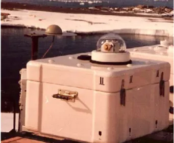
The objective of the present study is to apply the same technique to the Antarctic total ozone observations for the yearly evaluation of ozone depletion. In order to estimate the loss, we use ground-based measurements from three SAOZ stations in the Antarctic. Figure 1 shows the oldest SAOZ instrument installed in the Antarctic in 1988. Further, we use measurements from six Dobsons, two Brewers and a UV-VIS (Ultra Violet–Visible) DOAS (Differential Optical Ab-sorption Spectroscopy) spectrometer that includes observa-tions from the historical staobserva-tions Halley, Syowa, and South Pole. Table 1 and Fig. 2 show details of the stations. We use the REPROBUS and SLIMCAT global three-dimensional (3-D) CTMs for the tracer simulations. The ozone loss de-rived from the ground-based measurements are compared to that of the space-borne observations of the Ozone Mon-itoring Instrument (OMI) on Aura and the Scanning Imag-ing Absorption Spectrometer for Atmospheric Chartography (SCIAMACHY) on ENVISAT.
We organise the article as follows: The introduction is followed by the description of ozone measurements used in this study in Sect. 2. Section 3 presents the models and the ozone loss estimation method. Section 4 details the
appli-Fig. 1. The SAOZ instrument at Dumont d’Urville in the Antarctic.
cation of the method to recent Antarctic measurements and Sect. 5 gives a brief discussion on total ozone in the southern high and mid-latitudes with respect to the ozone loss analy-ses. Section 6 concludes the study.
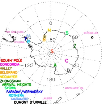
Fig. 2. The ground-based stations in the Antarctic and southern mid-latitudes considered in the ozone loss analyses. The mid-latitude stations are shown in light pink colour. The positions of Antarctic stations are marked by the first letter of their names in respective colours.
2 Ozone column observations 2.1 Ground-based
2.1.1 SAOZ
The zenith sky SAOZ UV-VIS spectrometers (Pommereau and Goutail, 1988) operate at 300–650 nm, looking at sun-light scattered from the zenith sky during twisun-light. Ozone is measured in the Chappuis band (450–650 nm) at high SZA between 86 and 91◦ every morning and evening. As con-cluded from various inter-comparison exercises (Roscoe et al., 1999; Vaughan et al., 1997), the measurements from dif-ferent SAOZ instruments are consistent within ±3%. The main source of uncertainty in the measurements is the air mass factor (AMF) and for instance, the difference in AMF between inside and outside the ozone hole can be up to 10%. 2.1.2 DOAS
This is a similar instrument to SAOZ but with differences of detail, e.g. light is collected by a small telescope and fed to the spectrograph using two depolarising quartz fibre bundles. The spectrograph consists of a UV and a visible channel. Ozone measurements are performed in 490–555 nm at 84– 90◦SZA, similar to SAOZ. Ozone slant column densities are converted using AMFs estimated from AMFTRAN Monte Carlo Radiative Transfer Model. The accuracy of ozone ver-tical column density retrieved from the Neumayer DOAS is
about 2%. The DOAS measurements are described in detail by Frieß et al. (2005).
2.1.3 Dobson spectrophotometer
The instrument consists of a double prism monochromator to measure the differential absorption of ozone in UV (Dobson, 1957). Individual measurements are performed by looking at the direct sun by clear sky and are averaged to a daily mean. Nevertheless, those measurements are limited to SZA <80◦ i.e. after mid-August at the polar circle. As the instrument re-quires calibration, comparison with the well-calibrated Dob-son #83 (Boulder, USA) is carried out. However, calibration with this instrument may not be accurate at the South Pole (because of high latitude and large SZA) and hence, it may slightly affect the accuracy of measurements. The estimated relative error in direct sun total ozone measurements is 0.5% or 1 DU (Basher, 1982).
2.1.4 Brewer spectrophotometer
Brewer measurements also make use of differential absorp-tion in the UV region (Brewer, 1973). The determinaabsorp-tion of total ozone is similar, but sensitivity of the instrument is better than that of the Dobson. As in the case of the Dob-son, an empirical relation between simultaneous direct sun and zenith sky has to be established if zenith observations are to be taken. Calibration of the instrument is essential. A well calibrated Brewer direct sun measurement has an error comparable to that of the Dobson.
2.2 Space-borne 2.2.1 OMI on Aura
The OMI sensor on the Aura satellite began to operate in 2004 as a successor to the Total Ozone Mapping Spectrom-eter (TOMS) (Levelt et al., 2006). The nadir viewing UV-VIS spectrometer measures solar light scattered by the atmo-sphere with a spatial resolution at nadir of 13×24 km. The sun-synchronous orbit of Aura and the wide viewing angle of OMI enable daily global coverage of the sunlit portion of the Earth. The overpass data, spatial averages within 100 km, are retrieved using the TOMS v8 algorithm. The retrieval makes use of two wavelengths: 331.2 and 360 nm for high ozone and at high SZA. However, retrievals from 317.5 and 331.2 nm are used for most conditions. The uncertainty of the ozone column is 2–5% for SZA <84◦(Bhartia and
Welle-meyer, 2002).
2.2.2 SCIAMACHY on ENVISAT
SCIAMACHY (hereafter SCIA), an imaging spectrometer on board ENVISAT placed into orbit in 2002, utilises nadir, limb and sun/moon occultations for ozone column retrievals (Bovensman et al., 1999). The data are recorded from the
transmitted, back scattered and reflected solar radiation from the atmosphere at 240–1700 nm. The instantaneous field of view spans 2.6 km in the vertical and 110 km in the hori-zontal direction at the tangent point. We consider the total column overpass data calculated from nadir measurements, averaged within 100 km radius above each station, retrieved using the v2 algorithm based on TOSOMI (Total Ozone re-trieval scheme for SCIAMACHY based on the OMI DOAS algorithm). The estimated accuracy of the ozone column is about 2–3.3% (Eskes et al., 2005).
3 Estimation of ozone loss
To find chemical ozone depletion from the measurements by applying the passive technique, tracer calculation by a CTM is required. For this purpose, passive ozone (ozone calculated without interactive chemistry) simulations from REPROBUS for 2006–2009 and SLIMCAT for 2005 are considered, as the data from the former was not available in 2005. We use the diurnal averages of the ozone and tracer column simula-tions sampled at the location of each station. Nevertheless, a detailed discussion on the model calculations is beyond the scope of this study as it focuses on the method and measure-ments. The details of tracer simulations in the models are given in the following sections and the method is described afterwards.
3.1 REPROBUS
The REPROBUS 3-D CTM has been widely utilised in previ-ous studies of stratospheric chemistry (Lef`evre et al., 1994, 1998). It uses a hybrid σ -pressure vertical coordinate for which winds and temperatures are driven by the ECMWF op-erational data on 60 vertical levels to 0.1 hPa (∼60 km) until February 2006, and then 91 levels to 0.01 hPa (∼90 km) af-terwards. Vertical advection is computed directly from the analysed winds. The simulations presented here were inte-grated on a global grid with a horizontal resolution of 2◦×2◦. Chemical species are transported by a semi-Lagrangian code (Williamson and Rasch, 1989). The model includes a com-prehensive description of stratospheric chemistry. Absorp-tion cross-secAbsorp-tions and kinetics data are based on Sander et al. (2006). However, absorption cross sections of Cl2O2are
taken from Burkholder et al. (1990) and are extrapolated to 450 nm. Monthly varying H2SO4fields, leading to the
for-mation of liquid aerosols in the CTM, are computed from the outputs of a 2-D-model long-term simulation that consider impacts of volcanic eruptions. The model includes reactions on binary and ternary liquid aerosols as well as on water-ice particles. The composition of liquid aerosols is calcu-lated analytically (Luo et al., 1995). The ice particles are assumed to incorporate HNO3in the form of nitric acid
tri-hydrate (NAT) (Davies et al., 2002). Clyand Bryare
explic-itly calculated from their long-lived sources at the surface
and are therefore time dependent. An additional 6 pptv of bromine in the form of CH2Br2is added to Bryto represent
the contribution of brominated short lived species reaching the stratosphere (WMO, 2007).
3.2 SLIMCAT
SLIMCAT is an off-line 3-D CTM described in detail by Chipperfield (1999). The model uses hybrid σ -θ as the ver-tical coordinate and extends from the surface to a top level which depends on the domain of the forcing analyses (Feng et al., 2007a). Here the horizontal winds and temperatures are specified using ECMWF operational data of 60 vertical levels to 0.1 hPa. Vertical advection in the θ -domain (above 350 K) is calculated from diabatic heating rates using the Na-tional Centre for Atmospheric Research Community Climate Model radiation scheme (Feng et al., 2005b; Chipperfield, 2006). Chemical tracers are advected by conservation of second-order moments (Prather, 1986). The model describes the main stratospheric chemical species Ox, HOx, NOy, Cly,
Bry as well as source gases and a treatment for CH4
oxi-dation. It contains a detailed gas-phase stratospheric chem-istry scheme. As in REPROBUS, the photochemical data are based on Sander et al. (2006) and the absorption cross sections of Cl2O2 are taken from Burkholder et al. (1990),
which are extrapolated to 450 nm. The model treats hetero-geneous reactions on liquid aerosols, NAT and ice (Chip-perfield, 1999), and denitrification schemes (Davies et al., 2002). An extra 6 pptv of bromine reaching the stratosphere from short-lived species is also included in the calculations (Feng et al., 2007b; WMO, 2007).
3.3 The passive tracer method
The ozone loss by the passive method is computed by sub-tracting passive ozone from measured ozone. Large changes in total ozone inside polar vortex are related to convergence or divergence due to changes in tropopause height, plane-tary wave induced adiabatic motions and diabatic descent due to radiative cooling. To find the ozone depletion in-side the vortex, the Nash et al. (1996) criterion is applied to find the vortex limit [maximum of the first derivative of potential vorticity (PV)]. A sensitivity test was conducted using the criterion of 35 PV units (pvu) and 45 pvu (1 pvu is 10−6Km2kg−1s−1). While the low PV criterion adds noise, the high PV criterion makes the data sparse. As ex-pected, though there were differences in number of observa-tions inside the vortex when using different criteria, the final results were similar. Therefore, the Nash et al. (1996) crite-rion is adopted after exempting some apparent noise in the vortex limit data. The PV data used to differentiate the vor-tex measurements were generated from the MIMOSA con-tour advection model (Hauchecorne et al., 2002) forced by the ECMWF meteorological analyses.
120 150 180 210 240 270 300 330 360 Day of year 2007 0 200 400 600 Ozone (DU) OMI ozone SCIA ozone SAOZ ozone
SLIMCAT passive ozone REPROBUS passive ozone
MAY JUN JUL AUG SEP OCT NOV DEC
-60 -50 -40 -30 -20 -10 PV (pvu) Vortex Edge PV
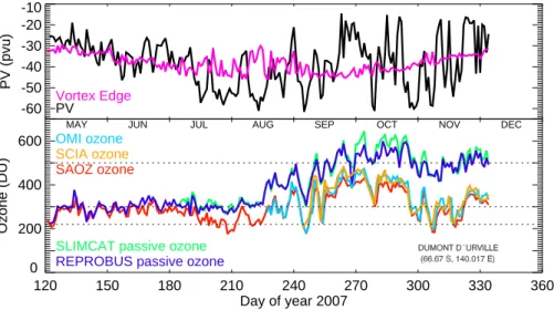
Fig. 3. Temporal evolution of various parametrs used for the computation of ozone loss at Dumont d’Urville in 2007. Top: ECMWF potential vorticity at 475 K (black), and polar vortex edge (magenta). Bottom: SAOZ (red), OMI (cyan) and SCIA (yellow) daily mean total ozone and SLIMCAT (green) and REPROBUS (blue) passive ozone (tracer). The horizontal bars represent the 220 DU ozone hole criterion, the 300 DU average pre-ozone hole value, and the 500 DU average spring column in the absence of depletion.
The vortex edge calculated at 475 K, where the concentra-tion of ozone has its maximum in spring, is selected for its loss estimation. The ozone loss analysis starts in July and it extends until November.
Figure 3 illustrates the basics of the tracer scheme with relevant data at Dumont d’Urville for the winter 2007. The day-to-day variations due to vortex positions are well cap-tured by the measurements and simulations. From July on-wards, the ozone values inside the vortex decrease with time while they increase outside. The ozone columns, both mea-sured and calculated, are anti-correlated with the PV values, where the high PV corresponds to the low ozone in the vor-tex. The SAOZ observations are continuous throughout the winter at Dumont d’Urville, while both OMI and SCIA start in mid-August and thus miss the onset of ozone loss process. Nevertheless, the observations from both ground and space are very consistent afterwards.
The chemical ozone loss is then computed by finding the difference between the tracer simulated by the CTM and ozone measured from the ground or space. That is, the observed ozone loss in absolute unit (DU) is estimated as ozonemeas-tracer and in relative unit (%) is computed as
100×(ozonemeas-tracer)/tracer. This procedure is repeated
for each station and then sorted for inside the vortex. The example of 2007 is given in Fig. 4. The ozone loss starts at the edge of the vortex in early-July, when it is displaced to the sunlit latitudes. So the stations at the edge, such as Du-mont d’Urville and Rothera, are subjected to ozone loss early in the winter (e.g. Lee et al., 2000). As the day gets longer and light penetrates deeper inside the continent, the stations Concordia and Arrival Heights followed by Neumayer, Hal-ley, Syowa, Belgrano and South Pole undergo ozone
deple-tion (e.g. Chubachi, 2009). Measurements at the latter sta-tions were possible only in late-August or September. The figure clearly shows the late winter start of ozone depletion in the vortex core, Concordia in particular (South Pole mea-surements start even later, by mid-September, e.g. Solomon et al., 2005). This delayed onset also produces a step like fea-ture in the mean ozone loss curves in the July to mid-August period.
The intensity of ozone destruction is also connected to the position of the stations and axis of the vortex. For instance, the sites well inside the vortex experience more loss than those at the edge. Therefore, South Pole or Belgrano ob-serve more severe loss than Dumont d’Urville in each win-ter. The loss at Concordia is less than that of South Pole and larger than that of Dumont d’Urville due to the strength and longevity of the vortex over the respective locations.
The results delineate three distinct phases of the Antarctic ozone loss as marked with dotted vertical lines and colour shades in Fig. 4. The first stage starts in July and ends in late-September, where rapid loss occurs with return of the sun over the continent. The loss rate is largest in this pe-riod. Starting time of this phase varies from May to July depending on the temperature, the time of vortex forma-tion and its locaforma-tion. if the temperature is relatively cold and the vortex appears in early winter that shifted in lat-itude, there can be some loss in May–June and thus this phase may start in May. The cumulative maximum of the ozone loss is generally observed in early-October, afterwards the depletion stops when PSCs (Polar Stratospheric Clouds) are no longer forming because of comparatively higher tem-peratures. This is the second phase of the ozone loss pro-cesses, where depth of the ozone hole reduces then more or
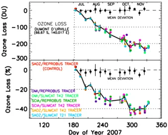
Fig. 4. Vortex averaged (ten-day mean) individual ozone loss esti-mated at the ground-based stations in the Antarctic using the passive method (top: DU, bottom: percent). The loss in absolute unit (DU) is estimated as ozonemeas-tracer and its relative loss (%) is
com-puted as 100×(ozonemeas-tracer)/tracer. The black thick lines
rep-resent the mean and the error bars reprep-resent the standard deviation from the mean. The observations from Kerguelen, a mid-latitude station, are not included in the average, shown with “x” marks. The vertical dotted lines represent the different phases of ozone loss pro-cesses in the Antarctic as marked in the colour shades (see text), while the horizontal dotted lines represent 50, 150 and 250 DU and 15, 30, 45 and 60% of ozone loss. Some stations start the win-tertime observation in August or September. The ozone loss onset varies with respect to sunlit latitudes and therefore, the onset period depends on co-ordinates of the stations. Thus, the onset and rapid loss phases are clustered together with dashed lines.
less slowly depending on vortex erosion, exchange with mid-latitudes, and location of the station. Therefore, the edge sta-tions, i.e. Dumont d’Urville, Marambio and Rothera, recover more rapidly. The ozone hole is not homogeneous. Depend-ing on the location of the station with respect to the vortex, the loss can vary within ±10% (±20 DU). In the third phase, the ozone hole disappears in general by the end of Novem-ber or early-DecemNovem-ber as in 2006, except in the case of the unprecedented vortex split in 2002. It is during this period (October–November) that vortex pieces or filaments more or less filled-in could be observed at lower latitudes as in Ker-guelen at 49◦S in present case.
3.4 Error analysis
In order to investigate the uncertainty of the method, ozone loss under various conditions are analysed. Figure 5 shows the ozone depletion estimated with SAOZ, OMI and SCIA using REPROBUS and SLIMCAT (with both T42 and T21 resolution) tracer for Dumont d’Urville in 2007. The stations at the edge region (Lee et al., 2000) show more spread than
Fig. 5. Vortex averaged (ten-day mean) ozone loss diagnosed using different measurements and various tracer calculations by differ-ent model setups at Dumont d’Urville (top: DU, bottom: percdiffer-ent). The loss in absolute unit (DU) is estimated as ozonemeas-tracer and
its relative loss (%) is computed as 100×(ozonemeas-tracer)/tracer.
The black solid lines represent the mean ozone loss from all sce-narios and the black filled-circles represent the average deviation from the control (SAOZ/REPROBUS tracer). The error bars rep-resent the standard deviation from the mean. The dotted vertical line represents 1 July. The dotted horizontal lines represent 100 and 200 DU and 20 and 40% of ozone loss.
those inside the vortex (for which Dumont d’Urville shows the largest). We use the SAOZ/ground-based ozone loss anal-ysis with REPROBUS tracer using Mimosa PV and Nash vortex edge as the control, since simulated results match well with the measurements. To compute the uncertainty, the difference between the control and the ozone loss was es-timated with other setups, as shown in the figure. The root sum square (RSS) of all these differences as well as the un-certainties in the measurements yield a deviation up to 4.4% (0–21 DU) depending on day.
The RSS computation includes all prime processes that af-fect the accuracy of the method. Those are: i) the system-atic differences between the instruments, drop in measured ozone due to presence of PSCs, and difference in AMF pro-file shapes (considered in the analysis by including the mea-surement uncertainties of respective instruments), ii) differ-ences in simulated profiles with measurements when ozone varies rapidly (considered in the analysis by using tracers from different models of varying horizontal and vertical res-olution), and iii) shifts in location of estimated vortex edge (considered in the analyses by testing with different vortex edge criteria, PV data sets and horizontal resolution of the models). Since size of the vortex can be smaller above the ozone loss analysis level of 475 K, air outside the vortex can-not be ruled out and was can-not possible to account for by these experiments.
3.5 Conclusions on the method
There are a few parameters that influence the strength of ozone loss evaluation method. The most evident are the re-alism of the tracer field in the models and the vortex edge calculation from potential vorticity. We tested how the de-rived ozone loss varies with the expected changes in these parameters. These tests were repeated for the overpass mea-surements from satellite observations. The RSS of the devia-tions including measurement accuracies is within 4%. Since accuracy of the measurements is in the order of 3–5% and the total error derived from RSS is ∼4%, the small contribu-tion from other input shows the consistency and potency of the method. In addition, the use of different model setups for the calculations of tracer ensures that the estimation provides consistent results and affirms that the method is sound. The main dispersion of loss computation comes from the inho-mogeneous distribution of ozone in the vortex, which ranges from ±2–10% at the beginning when only the edge stations are exposed to sunlight, to ±0–5% at the end when depletion has stopped.
4 Application of the method: Antarctic winters 2005– 2009
We now examine the variability of the Antarctic ozone loss between 2005 and 2009. The ozone loss analyses using SCIA observations exclude South Pole measurements be-cause of their unavailability. The daily ozone depletion rates are calculated in a common time window for all data sets, i.e. between day 225 and 275 in each winter. Figure 6 shows the ten-day boxcar average of the vortex mean ozone loss derived from the ground-based, OMI, SCIA and model (REPROBUS for the winters 2006–2009 and SLIMCAT in 2005) data for the recent winters and we begin the discussion with the most recent year. In order to preserve the temporal ozone loss features, instead of finding the vortex averaged depletion at each station in every ten days, the average of ozone and tracer data inside the vortex from all stations are considered here. Then the observed ozone loss in absolute unit (DU) is estimated as ozoneavg-traceravg and in relative
unit (%) is computed as 100×(ozoneavg-traceravg)/traceravg.
Here, the ozoneavg (traceravg) represents the mean of the
ozone (tracer) data inside the vortex from all stations. The same approach is repeated for the model simulations.
In 2009, the ozone depletion started by the first week of July and it peaked to 53% by late-September. The satel-lite observations, both OMI and SCIA, agree well with the ground-based analysis. The ozone loss rate shows 0.62 for ground-based, 0.58 for OMI, 0.54 for SCIA and 0.55%/day for the model. Further details of the analyses are listed in Table 2.
In 2008, the ground-based measurements find the ozone loss onset in early July and its maximum in early
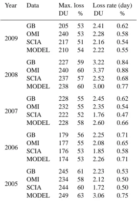
Octo-Table 2. Vortex averaged ozone loss (ten-day boxcar aver-age) estimated from the ground-based (GB), OMI and SCIA-MACHY (SCIA) observations and the total column integrated from REPROBUS (2006–2009) and SLIMCAT (2005) simulations (MODEL), during recent Antarctic winters. Extrapolated data are used for day 225 to calculate the ozone loss rates in 2007 and 2009 from SCIA.
Year Data Max. loss Loss rate (day)
DU % DU % GB 205 53 2.41 0.62 2009 OMI 240 53 2.28 0.58 SCIA 217 51 2.16 0.54 MODEL 210 54 2.22 0.55 GB 227 59 3.22 0.84 2008 OMI 240 60 3.37 0.88 SCIA 237 57 2.52 0.68 MODEL 238 60 3.00 0.77 GB 228 55 2.45 0.62 2007 OMI 232 55 2.35 0.54 SCIA 222 52 1.76 0.47 MODEL 228 58 2.60 0.66 GB 179 56 2.25 0.71 2006 OMI 177 55 2.08 0.65 SCIA 176 53 1.85 0.58 MODEL 174 53 2.26 0.71 GB 245 61 2.23 0.53 2005 OMI 234 58 2.12 0.50 SCIA 244 60 1.72 0.50 MODEL 249 63 3.06 0.75
ber, about 59%. Similar results are found in the loss com-puted from satellite and model data, where the differences are within ±2%. The loss rates analysed from the measurements and simulations exhibit similar values of about 0.8%/day, but slightly less from the SCIA observations.
In 2007, as found in other winters, the depletion started in July and reached its peak by mid-October. The loss derived from ground-based and OMI observations exhibit a similar maximum of ∼55%, whereas it is 3% less with SCIA and 3% more with the model. The ozone depletion rates computed from different data sets show 0.62 for ground-based, 0.54 for OMI, 0.47 for SCIA and 0.66%/day for the model.
In 2006, the observed ozone depletion shows its onset in early July. The maximum loss derived from ground-based observations shows 56% by early October, consis-tent with that of OMI measurements. The loss computed from the SCIA and model data show slightly lower values of about 53%. The simulated loss in July–September is slightly smaller than that of the ground-based observations, even if both return similar loss rates of 0.71%/day.
In 2005, a large loss was measured in early winter and its maximum in early-October. The peak depletion derived
Fig. 6. Vortex averaged (ten-day boxcar average) ozone loss estimated from the ground-based (GB) measurements (as listed in the plots) in red, the OMI observations in blue (OMI), the SCIAMACHY measurements in dark yellow (SCIA) and the model simulations by REPROBUS in 2006–2009 and SLIMCAT in 2005 in green (MODEL) for the Antarctic winters 2005–2009 (Left: percent, right: DU). The loss in absolute unit (DU) is estimated as ozoneavg-traceravg and its relative loss (%) is computed as 100×(ozoneavg-traceravg)/traceravg. The
ozoneavg/traceravgrepresents the average of the measurements/simulations inside the vortex from all stations. The SCIA average excludes
South Pole measurements due to unavailability. The dotted vertical lines represent day 182 (1 July), and day 225 and 275, the time window used for the computations of daily ozone loss rates. The horizontal lines represent 15, 30, 45 and 60%, and 50, 150 and 250 DU.
from the ground-based measurements is 61%, whereas it is 1% more from the model calculations. The loss evaluated from satellite observations find agreeable results within ±2-5%. The estimated loss rates are 0.53, 0.5, 0.5 and 0.75%/day for ground-based, OMI, SCIA and SLIMCAT respectively.
5 Inter-annual variability
In this section, we discuss the inter-annual variability of ozone loss and ozone in the southern high and mid-latitudes. The passive method used for the estimation of ozone loss de-pends largely on tracer simulations in the models. Therefore,
a survey with ozone column measurements is necessary to analyse the consistency of the loss evaluation. Since mea-surements are available for decades, this diagnosis is not re-stricted to 2005–2009, as in the case of ozone loss estimation. However, a rigorous statistical analysis, for instance, as done by Vyushin et al. (2007) for the high latitudes or Andersen and Knudsen (2006) for the northern mid-latitudes, is beyond the scope of this work and will not be attempted.
5.1 Antarctic ozone loss
The general behaviour of ozone loss with time and chemistry is alike in all winters. However, the cumulative loss, period
of maximum depletion and longevity of the ozone hole al-ter in accordance with the strength of the vortex. In general, as found in previous studies the Antarctic ozone depletion starts in early-July and stops during the last week of Septem-ber (Solomon et al., 2005; Tilmes et al., 2006; Huck et al., 2007) except in 2006 when it extended until the first week of October. In all years the ozone hole could be followed until the 3rdand 4t hweek of November (Bevilacqua et al., 1997; Solomon et al., 2005).
Figure 7 illustrates the daily minimum temperature from ECMWF within 50–90◦S at 475 K for 2005–2009. In gen-eral, temperatures below the formation of NAT (TNAT) are
found from mid-May until October. Temperatures below the freezing point of water-ice (TICE) occur from June to
late-September. Among the last four winters, 2007 shows the lowest temperatures in May–June, 2008 shows the lowest in July to August and 2006 shows the lowest in mid-September to November. The recent winter 2009 was gener-ally colder than 2008 and 2005, while the winter 2007 had the warmest September–November and earliest vortex dissi-pation. The winter 2006 was one of the coldest, in which the breakdown of the vortex was observed in December.
As expected from their similar temperatures, the cold win-ters 2006, 2008 and 2009 show little difference in ozone loss. The maximum ozone loss was found early in 2006 as compared to other winters because of the colder tempera-tures and well formed early vortex, whereas the warm winter 2007 shows relatively lower loss. The ozone loss evalua-tion from the ground and space is very consistent, showing small differences, within±2%. The model calculations also find similar scales of ozone depletion in each winter, where the differences with observations are about ±3–5%. Though the deviations are small, the geographical differences in sam-pling among the ground-based, satellite and the model data could also contribute to this offset. When compared to other winters, the loss calculated from the model underestimates the measured loss in 2006. There were no changes in the model run input other than the ECMWF meteorological data used in this year as compared to other years. Therefore, the differences could be due to the possible inaccuracies in the temperature data [e.g. Boccara et al. (2008); Pitts et al. (2007)], which in turn affect PSCs, chlorine activation and hence, ozone calculations by the model.
There are no other ozone loss estimations available for the Antarctic winters 2005–2009 to compare with our re-sults. The available studies for the previous winters are not directly comparable as they use either partial columns or a different evaluation method. However, as concluded in WMO (2007) and references therein, it is clear that Antarc-tic ozone depletion has stabilised in the 1995–2005 decade because of its saturation, i.e. due to the complete destruc-tion of ozone over a broad vertical layer in the lower strato-sphere. Therefore, most of the inter-annual variability results more from levels of dynamic forcing than a change in lev-els of Equivalent Effective Stratospheric Chlorine (EESC)
Fig. 7. ECMWF daily minimum temperatures within 50–90◦S at 475 K for 2005–2009. The horizontal lines represent the TNATand
TICEthresholds. The dotted vertical line represents 1 July.
[e.g. Yang et al. (2008)]. The amplitudes of total loss re-ported in 1995–2005 are very similar to that derived in 2005– 2009. For instance, the partial column loss estimated at 350–600 K from Improved Limb Atmospheric Spectrometer (ILAS) measurements by applying the tracer correlation ap-proach was 157±17 DU in early-October 2003 (Tilmes et al., 2006), which is close to our evaluation for the recent win-ters during the same period. Our conclusion on the inter-annual variability of ozone loss is also in line with the pre-vious studies (Hofmann et al., 1997; Wu and Dessler, 2001; Bevilacqua et al., 1997; Solomon et al., 2005; Hoppel et al., 2005; Lemmen et al., 2006; Huck et al., 2007). The stud-ies based on ozonesonde observations (for e.g. South Pole and Syowa) in the Antarctic have some significance in this context as we have used measurements from these stations for our evaluations [e.g. Hofmann et al. (1997); Solomon et al. (2005)]. Additionally, the ozone loss rates in Septem-ber derived from the South Pole ozone soundings in 1990s (Hofmann et al., 1997) and that estimated from the SLIM-CAT simulations in early 2000s (Feng et al., 2005a) are re-spectively 2–3 and 2.6–3.2 DU/day. The loss rates found in our study are also by the same order of magnitude (2– 3 DU/day or 0.6–0.9%/day), which reiterates the small inter-annual variability of the Antarctic ozone loss.
5.2 Southern high latitude total ozone
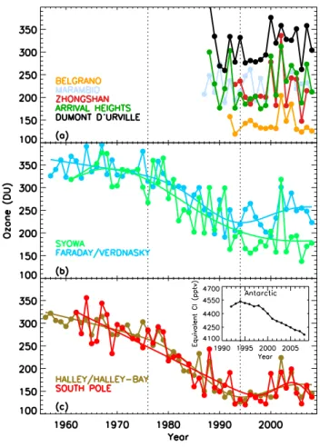
Figure 8 displays the October mean of total ozone from var-ious stations together with EESC in the Antarctic. The four historic stations Halley, Syowa, South Pole and Faraday have measurements since 1956. These observations show large decrease in total column ozone until early 1990s and satu-ration of the loss afterwards (WMO, 2007). The little inter-annual variation due to the saturation is clearly evident after mid-nineties. These results are in very good agreement with previous works on total ozone trends in the Antarctic (Bojkov and Fioletov, 1995; Bojkov et al., 1995; Bodeker et al., 2001; Fioletov et al., 2002; Kane, 2008). The above-mentioned
Fig. 8. Evolution of October mean total ozone in the Antarctic from ground-based observations. (a) Stations installed after 1985, (b) historical stations Syowa and Faraday, and (c) historical stations South Pole and Halley and the equivalent chlorine in the Antarctic in the inset. The historical data are plotted separately for clarity reasons. The dotted vertical lines represent years 1976 and 1994. A Gaussian fit is shown in the time series of the historical stations.
works are especially noteworthy here as we also present sim-ilar results for South Pole, Syowa, Halley and Faraday, and thus a very consistent evaluation of inter-annual variation of total ozone in the Antarctic. Even if the current negative trends in EESC sustain in the coming years, studies indicate that it will take several decades to appear ozone recovery sig-nals in the Antarctic (e.g. Vyushin et al., 2007; Yang et al., 2008).
5.3 Southern mid-latitude total ozone
The ozone loss analysis for the Antarctic would not be com-plete without assessing its impact on mid-latitudes. There-fore, we now examine the ozone loss computed above three stations located at three different regions in southern mid-latitudes. This diagnosis is particularly important since very low ozone of around 250 DU was observed on some days at these stations during recent winters. Figure 9 shows the
Fig. 9. Ozone loss estimated during the vortex events at selected southern mid-latitude stations for the recent Antarctic winters (Top: DU, bottom: percent). The loss in absolute unit (DU) is esti-mated as ozonemeas-tracer and its relative loss (%) is computed as
100×(ozonemeas-tracer)/tracer. The dotted vertical line represents
July 1, and the horizontal lines show 50 and 150 DU and 15, 30 and 45% of ozone loss.
ozone loss estimated from Rio Gallegos, Kerguelen and Mac-quarie Island ozone measurements in 2005–2009. Extension of the vortex to the mid-latitudes was absent in some years, as in 2005 at Macquarie Island and in 2008 at Kerguelen. Fur-ther, there were no vortex events found over Lauder during recent winters.
The analyses expose the vortex overpasses for a few days in October 2008 and November 2009 and show a maximum ozone loss of 40–45% (150–200 DU) at Rio Gallegos. A similar scale (30–50%) of reduction from a higher number of vortex occurrences at Ushuaia is also estimated with the SLIMCAT tracer in September–November 2004–2008 (not shown). Except in 2008, about 30% (50–100 DU) of ozone depletion is observed at Kerguelen during the vortex events in October–November of the recent winters. Conversely, pas-sage of the vortex over Macquarie Island was found mostly during early winter and the observed ozone loss was about 10–20% (up to 100 DU) in 2006–2009. Nevertheless, this is equal to that of the Antarctic during the same period.
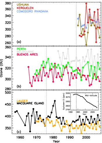
In order to analyse the inter-annual variations, the October mean of the total ozone from selected mid-latitude stations are examined in Fig. 10. There is a weak signal of ozone reduction (∼50 DU) in 1975–1993 at Lauder and Macquarie Island, in agreement with previous studies of Harris et al. (2003) for the former and Chubachi (2009) for the latter. The measurements at Perth and Buenos Aires also show some reduction in ozone during the period (Kane, 1991, 2008).
Fig. 10. Evolution of October mean total ozone from southern mid-latitude ground-based stations (a) stations installed after 1985, (b) historical stations at 30–40◦S, and (c) historical stations at 40– 60◦S with equivalent chlorine in the mid-latitude in the inset. The dotted vertical lines represent years 1976 and 1994.
These results are consistent with the well established mean 5% depletion in the southern mid-latitudes since the pre-ozone hole period (WMO, 2007). Nevertheless, the time se-ries of Melbourne is too short to deduce a significant trend. As expected, the measurements at Ushuaia, Comodoro Riva-davia and Kerguelen exhibit large inter-annual variations due to the episodic vortex exposures.
6 Conclusions
The passive method is shown to provide ozone loss estima-tions within an accuracy of about 4% and is applied to eval-uate ozone loss from the ground-based measurements in the Antarctic winters 2005–2009. The depletion is shown to start at the edge of the vortex by July in every winter and each station shows different timing for the onset of ozone loss depending on its exposure to sunlight. Further, the magni-tude of loss is also different at each station in line with the temperature, PV, PSCs, and prevailing heterogeneous
chem-istry, which is quite in agreement with our current under-standing of polar wintertime chemistry. In accordance with previous studies, the ground-based stations show substantial ozone loss of around 55% since 2005. However, the year-to-year differences in ozone loss are not large in the Antarctic, consistent with earlier studies. The ozone loss and loss rates computed from OMI and SCIA observations compare well with that of the ground-based measurements (within ±2%). The CTMs imitate well the ozone depletion features and re-produce the maximum loss within ±3% difference.
The October average of the total column measurements at the historical ground-based stations do show that the deple-tion started in the late 1970s. The ozone reducdeple-tion peaked in the early 1990s and stabilised afterwards until present due to its saturation. The analyses indicate no clear sign of sig-nificant ozone recovery yet. Another important feature is the effect of the ozone hole at southern mid-latitudes. The SAOZ measurements at Kerguelen and Rio Gallegos, the first obser-vations from the latter, reveal severe ozone loss (20–45% or 50–200 DU) episodes, which reiterates the value of observa-tions in southern mid-latitudes.
This study shows that, the maintenance of an efficient ground-based network independent of satellites, particularly UV-VIS that are capable of making observations in early-winter, is inevitable for monitoring the long term evolution of the ozone hole and its anticipated recovery from the re-duced chlorofluorocarbon (CFC) emissions.
Acknowledgements. We thank Udo Frieß of Institute for Envi-ronmental Physics, Uni-Heidelberg, Germany for the Neumayer data, Jonathan Shanklin, British Antarctic Survey (BAS) for the BAS Antarctic stations data, Eric Nash of NASA GSFC for the vortex edge data, Cathy Boonne of Centre for Atmospheric Chemistry Products and Services (ETHER) for providing with MIMOSA PV and REPROBUS ozone and tracer data, and Eduardo Quel, Elian Wolfram and, Jacobo Salvador of CEILAP (CITEFA-CONICET) for the Rio Gallegos data. The participation of BAS in this study is part of BAS’s Polar Science for Planet Earth programme, funded by the Natural Environment Research Council of UK. The OMI data are retrieved from Aura Validation Data Center of NASA (http://avdc.gsfc.nasa.gov) and the SCIAMACHY data obtained from TEMIS web interface (http://www.temis.nl). The EESC data for the Antarctic and mid-latitudes were obtained from NOAA website (http://www.esrl.noaa.gov/gmd/odgi/). The data used in this publication were obtained as part of the Network for the Detection of Atmospheric Composition Change (NDACC) and are publicly available (see http://www.ndacc.org). The French stations are supported by IPEV (Institut Paul Emile Victor), INSU (Institut des Sciences de l’Univers) and CNES (Centre National d’Etudes Spatiales). A good part of the data used in this work is also taken from World Ozone and Ultraviolet Radiation Data Centre (WOUDC) and are publicly available (see http://www.woudc.org). We take this opportunity to thank the respective national governing bodies, research establishments and station scientists, who maintain the stations. The work was supported by a funding from French ANR/ORACLE and EC/SCOUT-O3projects.
The publication of this article is financed by CNRS-INSU.
References
Andersen, S. B. and Knudsen, B. M.: The influence of polar vor-tex ozone depletion on NH mid-latitude ozone trends in spring, Atmos. Chem. Phys., 6, 2837–2845, doi:10.5194/acp-6-2837– 2006, 2006.
Basher, R. E.: Review of the Dobson spectrophotometer and its accuracy, WMO Global Ozone Research and Monitoring Project, Report No. 13, WMO, Geneva, 1982.
Bevilacqua, R. M., Debrestianet, D. J, Aellig, C. P., et al.: POAM II ozone observations in the Antarctic ozone hole in 1994, 1995, and 1996, J. Geophys. Res., 102(D19), 23643–23657, doi:10.1029/97JD01623, 1997.
Bhartia, P. K. and Wellemeyer, C. W.: TOMS-V8 total O3
al-gorithm, NASA Goddard Space Flight Centre, Greenbelt, MD, OMI Algorithm, Theoretical Basis Document Vol. II., 2387 pp., 2002.
Boccara, G., Hertzog, A., Basdevant, C., and Vial, F.: Accuracy of NCEP/NCAR reanalyses and ECMWF analyses in the lower stratosphere over Antarctica in 2005, J. Geophys. Res., 113, D20115, doi:10.1029/2008JD010116, 2008.
Bodeker, G. E., Scott, J. C., Kreher, K., and McKenzie, R. L.: Global ozone trends in potential vorticity coordinates us-ing TOMS and GOME inter-compared against the Dobson network: 1978–1998, J. Geophys. Res., 106, 23029–23042, doi:10.1029/2001JD900220, 2001.
Bojkov, R. D., and Fioletov, V. E.: Estimating the global ozone char-acteristics during the last 30 years, J. Geophys. Res., 100(D8), 16537–16551, doi:10.1029/95JD00692, 1995.
Bojkov, R. D., Bishop, L., and Fioletov, V. E.: Total ozone trends from quality-controlled ground-based data (1964–1994), J. Geo-phys. Res., 100(D12), 25867–25876, doi:10.1029/95JD02907, 1995.
Bovensman, H., Burrows, J. P., Buchwitz, M., Frerick, J., No¨el, S., Rozanov, V. V., Chance, K. V., and Goede, A. P. H.: SCIA-MACHY: mission objectives and measurement modes, J. Atmos. Sci., 56, 127–150, 1999.
Brewer, A. W.: A replacement for the dobson spectrophotometer?, Pure Appl. Geophys., 919(1136), 106–108, 1973.
Burkholder, J. B., Orlando, J. J., and Howard, C. J.: Ultraviolet absorption cross-sections of Cl2O2between 210 and 410 nm, J. Phys. Chem., 94, 687–695, 1990.
Chipperfield, M. P.: Multiannual simulations with a Three-Dimensional chemical transport model, J. Geophys. Res., 104, 1781–1805, 1999.
Chipperfield, M. P.: New version of the TOMCAT/SLIMCAT off-line chemical transport model: Inter-comparison of stratospheric tracer experiments, Q. J. Roy. Meteorol. Soc., 132, 1179–1203, doi:10.1256/qj.05.51, 2006.
Chubachi, S.: Seasonal start of the Antarctic ozone hole derived from observations with Dobson spectrophotometers, Int. J. Re-mote Sens., 30, 3907–3916, doi:10.1080/01431160902821957, 2009.
Davies, S., Chipperfield, M. P., Carslaw, K. S., and et al.: Modelling the effect of denitrification on Arctic ozone deple-tion during winter 1999/2000, J. Geophys. Res., 107, 8322, doi:10.1029/2001JD000445, 2002.
Dobson, G. M. B.: Observer’s handbook for the ozone spectropho-tometer, Ann. Int. Geophys. Year 5, 46–89, 1957.
Eskes, H. J., van der A. R. J., Brinksma, E. J., Veefkind, J. P., de Haan, J. F., and Valks, P. J. M.: Retrieval and validation of ozone columns derived from measurements of SCIAMACHY on En-visat, Atmos. Chem. Phys. Discuss., 5, 4429–4475, 2005, http://www.atmos-chem-phys-discuss.net/5/4429/2005/. Farman, J. C., Gardiner, B. G., and Shanklin, J. D.: Large losses of
total ozone in Antarctica reveal seasonal ClOx/NOxinteraction,
Nature, 315, 207–210, 1985.
Feng, W., M. P. Chipperfield, H. K. Roscoe, J. J. Remedios, A. M. Waterfall, G. P. Stiller, N. Glatthor, M. H¨opfner, D-Y. Wang: Three-Dimensional Model Study of the Antarctic Ozone Hole in 2002 and Comparison with 2000, J. Atmos. Sci., 62, 822–837, 2005a.
Feng, W., Chipperfield, M. P., Davies, S., Sen, B., Toon, G., Blavier, J. F., Webster, C. R., Volk, C. M., Ulanovsky, A., Ravegnani, F., von der Gathen, P., Jost, H., Richard, E. C., and Claude, H.: Three-dimensional model study of the Arctic ozone loss in 2002/2003 and comparison with 1999/2000 and 2003/2004, Atmos. Chem. Phys., 5, 139–152, doi:10.5194/acp-5-139-2005, 2005b.
Feng W., M. P. Chipperfield, S. Davies, P. von der Gathen, E. Kyro, C. M. Volk, A. Ulanovsky and G. Belyaev: Large chemical ozone loss in 2004/05 Arctic winter/spring, Geophys. Res. Lett., 34, L09803, doi:10.1029/2006GL029098, 2007a.
Feng, W. Chipperfield, M. P., Dorf, M., Pfeilsticker, K and P. Ri-caud: Mid-latitude ozone changes: Studies with a 3-D CTM forced by ERA-40 analyses, Atmos. Chem. Phys., 7, 2357–2369, doi:10.5194/acp-7-2357-2007, 2007b.
Fioletov, V. E., Bodeker, G. E., Miller, A. J., McPeters, R. D. and Stolarski, R.: Global and zonal total ozone variations estimated from ground based and satellite measurements: 1964–2000, J. Geophys. Res. 107(D22), 4647, doi:10.1029/2001JD001350., 2002.
Frieß, U., Kreher, K., Johnston, P. V., and Platt, U.: Ground-based DOAS measurements of stratospheric trace gases at two Antarc-tic stations during the 2002 ozone hole period, J. Atmos. Sci., 62, 765–777, 2005.
Goutail, F., Pommereau, J.-P., Phillips, C.. Deniel, C., Sarkissian, A., Lefevre, F., Kyro, E., Rummukainen, M., Ericksen, P., An-dersen, S., K˚astad Høiskar, B.-A., Braathen, G., Dorokhov, V., and Khattatov, V.: Depletion of column ozone in the Arctic dur-ing the Winters 1993–94 and 1994–95, J. Atmos. Chem., 32, 1– 34, 1999.
Harris J. M., Oltmans S. J., Bodeker G. E., Stolarski R., Evans R. D., and Quincy D. M.: Long-term variations in total ozone derived from Dobson and satellite data, Atmos. Environ., 37, 3167–3175, 2003.
Hauchecorne, A., Godin, S., Marchand, M., Heese, B., and Souprayen, C.: Quantification of the transport of chemical
con-stituents from the polar vortex to mid-latitudes in the lower stratosphere using the high-resolution advection model MI-MOSA and effective diffusivity, J. Geophys. Res., 107(D20), 8289, doi:10.1029/2001JD000491, 2002.
Hofmann, D. J., Oltmans, S. J., Harris, J. M., Johnson, B. J., and Lathrop, J. A.: Ten years of ozonesonde measure-ments at the south pole: Implications for recovery of spring-time Antarctic ozone, J. Geophys. Res., 102, 8931–8943, doi:10.1029/96JD03749, 1997.
Hoppel, K., Nedoluha, G., Fromm, M., Allen, D., Bevilac-qua, R., Alfred, J., Johnson, B., and K¨onig-Langlo, G.: Re-duced ozone loss at the upper edge of the Antarctic Ozone Hole during 2001–2004, Geophys. Res. Lett., 32, L20816, doi:10.1029/2005GL023968, 2005.
Huck, P. E., Tilmes, S., Bodeker, G. E., Randel, W. J., McDon-ald, A. J., and Nakajima, H.: An improved measure of ozone depletion in the Antarctic stratosphere, J. Geophys. Res., 112, D11104, doi:10.1029/2006JD007860, 2007.
Kane, R. P: Extension of Antarctic ozone hole to lower latitudes in the South American region, PAGEOPH, 135, 611–624, 1991. Kane, R. P: Is ozone depletion really recovering?, J. Atmos. Solar
Terr. Phys., 70, 1455–1459, 2008.
Lee, A. M., Roscoe, H. K., and Oltmans, S.: Model and measurements show Antarctic ozone loss follows edge of polar night, Geophys. Res. Lett., 27, 3845–3848, doi:10.1029/2000GL01144, 2000.
Lef`evre, F., Brasseur, G. P., Folkins, I., Smith, A. K., and Simon, P.: Chemistry of the 1991/1992 stratospheric winter: three di-mensional model simulation, J. Geophys. Res., 99, 8183–8195, 1994.
Lef`evre, F., Figarol, F., Carslaw, K. S., and Peter, T.: The 1997 Arctic ozone depletion quantified from three dimensional model simulations, Geophys. Res. Lett., 25, 2425–2428, 1998. Lemmen, C., Dameris, M., M¨uller, R., and Riese, M.: Chemical
ozone loss in a chemistry-climate model from 1960 to 1999, Geophys. Res. Lett., 33, L15820, doi:10.1029/2006GL026939, 2006.
Levelt, P. F., van den Oord, G. H. J., Dobber, M. R., Mlkki, A., Visser, H., de Vries, J., Stammes, P., Lundell, J., and Saari, H.: The Ozone Monitoring Instrument, IEEE T. Geosci. Remote Sens., 44, 1093–1101, 2006.
Luo, B., Carslaw, K. S., Peter, T., Clegg, S.L.: Vapour pressures of H2SO4/HNO3/HCl/HBr/H2O solutions to low stratospheric
temperatures, Geophys. Res. Lett., 22, 247–250, 1995.
Nash, E. R., Newman, P. A., Rosenfield, J. E., and Schoeberl, M. R.: An objective determination of the polar vortex using Ertel’s potential vorticity, J. Geophys. Res., 101, 9471–9478, 1996. Pitts, M. C., Thomason, L. W., Poole, L. R., and Winker, D. M.:
Characterization of Polar Stratospheric Clouds with spaceborne lidar: CALIPSO and the 2006 Antarctic season, Atmos. Chem. Phys., 7, 5207–5228, doi:10.5194/acp-7-5207-2007, 2007.
Pommereau, J.-P. and Goutail, F.: Stratospheric O3and NO2 Ob-servations at the Southern Polar Circle in Summer and Fall 1988, Geophys. Res. Lett., 15, 891–894, 1988.
Prather, M. J.: Numerical advection by conservation of second-order moments, J. Geophys. Res., 91, 6671–6681, 1986. Roscoe, H. K, Johnston, P. V., Van Roozendael, M., Richter, A.,
Preston, K., Lambert, J. C., Hermans, C., de Kuyper, W., Dze-nius, S., Winterath, T., Burrows, J., Sarkissian, A., Goutail, F., Pommereau, J.-P., et al.: Slant column measurements of O3
and NO2during the NDSC Intercomparison of zenith-sky UV-visible spectrometers in June 1996, J. Atmos. Chem., 32, 281– 314, 1999.
Sander, S. P., Friedl, R. R., Golden, D. M., et al.: Chemical kinetics and photochemical data for use in atmospheric studies, Eval. 15, JPL Publ. 06-2, Jet Propul. Lab., Pasadena, USA, 2006. Solomon, S., Portmann, R. W., Sasaki, T., Hofmann, D. J.,
and Thompson, D. W. J.: Four decades of ozonesonde mea-surements over Antarctica, J. Geophys. Res., 110, D21311, doi:10.1029/2005JD005917, 2005.
Tilmes, S., Mueller, R., Grooß, J.-U., Spang, R., Sugita, T., Naka-jima, H., and Sasano, Y.: Chemical ozone loss and related pro-cesses in the Antarctic winter 2003 based on Improved Limb Atmospheric Spectrometer (ILAS)-II observations, J. Geophys. Res., 111, D11S12, doi:10.1029/2005JD006260, 2006. Vaughan, G., Roscoe, H., Bartlett, K., and et al.: An
intercompar-ison of ground-based UV visible sensors of Ozone and NO2, J. Geophys. Res., 102, 1411–1422, 1997.
Vyushin, D. I., Fioletov, V. E., and Shepherd, T. G.: Impact of long-range correlations on trend detection in total ozone, J. Geophys. Res., 112, D14307, doi:10.1029/2006JD008168, 2007.
Williamson, D. L. and Rasch, P. J.: Two-dimensional semi-Lagrangian transport with shape-preserving interpolation, Mon. Weather Rev., 117, 102–129, 1989.
WMO (World Meteorological Organisation): The Global Atmo-sphere Watch Guide, WMO TD No. 553, 1993.
WMO (World Meteorological Organisation): Scientific assessment of ozone depletion: 2006, Global Ozone Research and Monitor-ing Project-Report No. 50, 572 pp., Geneva, Switzerland, 2007. Wu, J. and Dessler A. E.: Comparisons between measurements
and models of Antarctic ozone loss, J. Geophys. Res., 106(D3), 3195–3201, 2001.
Yang, E.-S., Cunnold, D. M., Newchurch, M. J., Salawitch, R., Mc-Cormick, J. M. P., Russell III, J. M., Zawodny, J. M., and Olt-mans, S. J.: First stage of Antarctic ozone recovery, J. Geophys. Res., 113, D20308, doi:10.1029/2007JD009675, 2008.