HAL Id: insu-02950993
https://hal-insu.archives-ouvertes.fr/insu-02950993
Submitted on 16 Dec 2020HAL is a multi-disciplinary open access
archive for the deposit and dissemination of sci-entific research documents, whether they are pub-lished or not. The documents may come from teaching and research institutions in France or abroad, or from public or private research centers.
L’archive ouverte pluridisciplinaire HAL, est destinée au dépôt et à la diffusion de documents scientifiques de niveau recherche, publiés ou non, émanant des établissements d’enseignement et de recherche français ou étrangers, des laboratoires publics ou privés.
Influence of the solar wind dynamic pressure on the ion
precipitation: MAVEN observations and simulation
results
Antoine Martinez, Ronan Modolo, François Leblanc, Jean-Yves Chaufray,
Olivier Witasse, N. Romanelli, Y. Dong, T. Hara, J. Halekas, R. Lillis, et al.
To cite this version:
Antoine Martinez, Ronan Modolo, François Leblanc, Jean-Yves Chaufray, Olivier Witasse, et al.. Influence of the solar wind dynamic pressure on the ion precipitation: MAVEN observations and sim-ulation results. Journal of Geophysical Research Space Physics, American Geophysical Union/Wiley, 2020, 125 (10), pp.e2020JA028183. �10.1029/2020JA028183�. �insu-02950993�
1
Influence of the solar wind dynamic pressure on the ion
1precipitation: MAVEN observations and simulation results.
2
A. Martinez 1, R. Modolo2, F. Leblanc1, J. Y. Chaufray 1,2, O. Witasse3, N. Romanelli4, Y. Dong5, T. Hara6,
3
J. Halekas7, R. Lillis6, J. McFadden6, F. Eparvier7, L. Leclercq8, J. Luhmann6, S. Curry6 and B. Jakosky7.
4 5
1 LATMOS/IPSL Sorbonne Université, UVSQ, CNRS, Paris, France
6
2 LATMOS/IPSL, UVSQ Université Paris-Saclay, Sorbonne Université, CNRS, Guyancourt, France
7
3 ESTEC, European Space Agency, Noordwijk, Netherlands
8
4 Solar System Exploration Division, NASA Goddard Space Flight Center, Greenbelt, MD, USA. CRESST
9
II, University of Maryland, Baltimore County, Baltimore, MD, USA. 10
5 Laboratory for Atmospheric and Space Physics, University of Colorado, Boulder, CO, USA
11
6 Space Science Laboratory, University of California, Berkeley, CA, USA
12
7 Department of Physics and Astronomy, University of Iowa, IA, USA
13
8 University of Virginia, Charlottesville, VA 22904, USA.
14 15 16
2 Abstract:
17
Using the data from the SWIA and STATIC instruments on board Mars Atmosphere and Volatile 18
EvolutioN (MAVEN) and LatHyS (Latmos Hybrid Simulation) simulations, we investigate the heavy ion 19
precipitation into the Martian atmosphere. We discuss the influence of the solar wind dynamic 20
pressure on the ion precipitation using observations performed by MAVEN from 04 June 2014 to 20 21
July 2017. The increase of the dynamic pressure from 0.63 to 1.44nPa is clearly associated with an 22
increase of the same order of magnitude of the precipitating oxygen ion energy flux measured by 23
MAVEN/STATIC from 9.9 to 20.6 × 10 eV. cm . sr . s at low energy (from 30 to 650 eV). In the 24
same way, from 650 eV to 25000 eV, MAVEN/SWIA (all species) observed an increase from 22.4 to 25
42.8× 10⁷eV. cm−2. sr−1. s−1 of the precipitating ion energy flux.
26
Performing two simulations using the average solar wind conditions for both solar dynamic pressure 27
regimes observed by MAVEN as input in the LatHyS model, we reproduce some of the key 28
characteristics of the observed oxygen ion precipitation. We characterize the oxygen ions simulated 29
by LatHyS by their energy and time of impact, their time of injection in the simulation and initial 30
position and the mechanism by which these ions were created. The model suggests that the main 31
cause of the increase of the heavy ion precipitation during an increase of the solar dynamic pressure 32
is the increase of the ion production by charge exchange, proportional to the increase of the solar wind 33
flux, which becomes the main contribution to the ion precipitation at high energy. 34
35 36
3 I. Introduction
37 38
In the absence of a global magnetic field, Mars’ upper atmosphere interacts directly with the solar 39
wind. Planetary neutral species (mainly carbon dioxide molecules, hydrogen and oxygen atoms) are 40
ionized by photoionization, electronic impact or charge exchange and are accelerated by the motional 41
electric field of the solar wind. These charged particles can precipitate into Mars’ atmosphere with 42
energy up to several keV and induce a cascade of collisions, transferring enough energy to atmospheric 43
particles to exceed the Martian escape velocity (Luhmann and Kozyra, 1991; Johnson, 1994). While 44
this process, named atmospheric sputtering, may have led to significant atmospheric escape in its early 45
history, as suggested by Luhmann et al. (1992), its contribution is nowadays minor compared to other 46
neutral escape processes like Jeans escape (Anderson and Hord, 1971; Krasnopolsky and Feldman, 47
2001) and photochemical escape (Lillis et al., 2015; 2017), or ion escape process like pick-up ions 48
(Luhmann, 1990; Fang et al., 2010; Dong et al., 2017) and ion outflow (Lundin et al., 1990; Andersson 49
et al., 2010). 50
Atmospheric escape induced by sputtering at the present epoch is expected to be small compared to 51
other mechanisms (Leblanc et al. 2017) and therefore difficult to quantify from direct measurements. 52
However, since heavy planetary ion precipitation (which we define as having mass larger or equal to 53
the mass of carbon atom) is the primary driver of atmospheric sputtering (Johnson et al, 2000; Wang 54
et al, 2014; 2015), it is essential to constrain the dependence of the precipitating ion flux on present 55
solar wind conditions in order to, potentially, extrapolate the effect of this mechanism, over the 56
Martian history. In situ measurements of precipitating ions began with Mars Express (MEX) spacecraft, 57
in orbit around Mars since December 2003, (e.g., Chicarro et al., 2004; Barabash et al., 2006). Hara et 58
al. (2011) reported that MEX observed enhancements of precipitating heavy ions (e.g. 𝑂 and 𝑂 ) 59
during the passage of Corotating Interaction Region (CIR) solar wind structures. This observation 60
suggests that heavy ion precipitation is highly variable and depends on the upstream solar wind 61
4 conditions at Mars. Thanks to Mars Atmosphere and Volatile EvolutioN (MAVEN) measurements, 62
observations of heavy ion precipitation during quiet solar wind conditions have been reported by 63
Leblanc et al. (2015), suggesting that atmospheric sputtering occurs almost continuously at Mars. 64
Several investigations, either from observational or modeling studies, have highlighted the influence 65
of the plasma properties on the Martian environment. Edberg et al. (2009), Hall et al. (2016), Halekas 66
et al. (2017) and Ramstad et al. (2017) have shown that the solar EUV irradiance and the solar wind 67
dynamic pressure have an influence on the position of plasma boundaries such as the Magnetic Pile-68
up Boundary (MPB) and the Bow Shock (BS). Indeed, the newly created exospheric ions can act to slow 69
the solar wind flux, which can move the bow shock position away from the planet (Hall et al, 2016). 70
Moreover, Lundin et al. (2008) also showed that the size of the Martian obstacle (estimated as 71
proportional to the BS position) influences the ion atmospheric escape rate. 72
The statistical study by Hara et al. (2017a) has showed that precipitating ion fluxes observed by MAVEN 73
(Jakosky et al., 2015) vary at least by an order of magnitude (typically between 10 𝑐𝑚 . 𝑠 𝑠𝑟 and 74
10 𝑐𝑚 . 𝑠 𝑠𝑟 for ions with energies higher than 25 eV) depending on the upstream solar wind 75
conditions such as the dynamic pressure, the magnitude of the interplanetary magnetic field, and the 76
motional electric field direction E⃗ = −V⃗ × B⃗ with V⃗ the solar wind velocity and B⃗ the 77
interplanetary magnetic field vector. Indeed, it has been shown by several theoretical studies 78
(Luhmann and Kozyra 1991; Chaufray et al. 2007; Curry et al. 2015) that the orientation of the motional 79
electric field may influence the energy and intensity of ion precipitation on Mars. These studies 80
suggested that the integrated total precipitating ion fluxes are globally larger in the –𝐸⃗ hemisphere 81
than in the +𝐸⃗ hemisphere. Pickup oxygen ions formed in the –𝐸⃗ hemisphere are accelerated towards 82
Mars and can precipitate while oxygen ions formed in the +𝐸⃗ hemisphere are accelerated away from 83
Mars and can escape. Such results have been observed by Martinez et al. (2019a) and Hara et al. 84
(2017a) thanks to MAVEN. 85
5 Curry et al. (2015) have studied the response of Mars O+ pickup ions to an ICME (March 8th, 2015) with
86
a test-particle approach and found that the oxygen ion precipitation depends on the phase of the ICME 87
with a maximum of precipitation during the shock. After the passage of the ICME shock, the 88
precipitating flux of the ejecta phase decreases but still remains greater than the precipitating flux 89
during the pre-ICME phase. Based on a similar approach, Fang et al. (2013) have shown that oxygen 90
ion precipitation can vary by at least one order of magnitude due to the variation in dynamic pressure 91
during ICME or CIR solar wind events. Similar conclusions have been reported by Hara et al. (2011) 92
with Mars Express observation or by Martinez et al. (2019a) with MAVEN observations during the 93
September 2017 solar events (Lee et al. 2018). 94
Complementary to observations, models can provide an extended set of information to better 95
characterize the physical processes under investigations. By being able to take into account a wide 96
variety of physical processes in time and space, models can be used to reproduce observations and 97
investigate the resulting mechanisms. They provide a three-dimensional context for the observations. 98
At the beginning of Martian exploration, with Mariner 4 or Phobos 2, computer simulations have been 99
found very useful for investigating the physic mechanisms of the atmospheric escape (Luhmann and 100
Kozyra, 1991; Luhmann, Jonhson & Zhang, 1992; Johnson, 1994; Leblanc & Johnson, 2001; 2002; 101
Dubinin & Lundin, 1995; Fang et al., 2010). Some studies also make it possible to model the present 102
and past contributions of these mechanisms to atmospheric escape (Chassefière & Leblanc, 2004). 103
Combining MEX observations and sophisticated global model simulations, Diéval et al. (2012) have 104
shown that the precipitating protons originate from both the solar wind and the planetary exosphere. 105
Here, we use model to simulate the potential effects of the solar dynamic pressure on the ion 106
precipitation. 107
In this paper, we further analyze the role of the solar dynamic pressure on the ion precipitation by 108
performing a detailed analysis of MAVEN measurements combined with the simulation of its potential 109
effects. The LATMOS Hybrid Simulation (LatHyS) model (Modolo et al, 2016) is used to constrain the 110
processes that may control the ion precipitation. The instruments and data used to perform this 111
6 analysis, as well as the methodology developed are described in section II. The model is described in 112
section III whereas section IV present the main results and lessons derived from the 113
simulation/measurement comparisons and section V the conclusions. 114
115
II. MAVEN measurements of the solar wind conditions and precipitating ion flux 116
A. Instruments and Data 117
The large set of MAVEN instruments (Jakosky et al. 2015) allows us to characterize the precipitating 118
ion flux as well as the upstream solar wind conditions and also to constrain the atmospheric and plasma 119
properties of the Martian environment. In this study, we use measurements performed by the Solar 120
Wind Ion Analyzer (SWIA; Halekas et al., 2015), the SupraThermal and Thermal Ion Composition 121
(STATIC; McFadden et al., 2015), the Magnetometer (MAG; Connerney et al., 2015a; 2015b) and the 122
Solar Extreme Ultraviolet Monitor (EUVM; Eparvier et al., 2015). The MAVEN/SWIA instrument is an 123
energy and angular ion spectrometer. In this work, we use the SWIA coarse survey data product, 124
covering an energy range between 25 eV/q and 25 keV/q with 48 energy steps logarithmically spaced, 125
a field of view (FOV) of 360° x 90° with 64 angular bins and 4s time resolution. The MAVEN/STATIC 126
instrument is an energy, mass and angular ion spectrometer. We used the STATIC “D1” data product, 127
covering an energy range between 0.1 eV/q and 35 keV/q with 32 energy steps logarithmically spaced, 128
a field of view (FOV) of 360° x 90° on 64 angular bins and 8 mass bins covering a mass range from 1 129
amu to 80 amu with a 4s time resolution. 130
We mainly based our study on MAVEN/SWIA despite the lack of mass resolution because 131
MAVEN/STATIC operates mostly in conic mode (McFadden et al. 2015) below 350 km in altitude 132
leading to a limited coverage for ions with energy larger than 650 eV. In the following, we use 133
MAVEN/STATIC to refine our analysis for energies below 650 eV. Moreover, in order to avoid any 134
potential bias in the measurement due to spacecraft charging, we only consider precipitating ions with 135
energies larger than 30 eV. Although MAVEN/SWIA does not have mass resolution, it can be used to 136
estimate the evolution of heavy ion precipitation for the high energy range. Pickup ions can be 137
7 accelerated by the motional electric field up to a maximum energy limit (Jarvinen and Kallio, 2014; 138
Rahmati et al., 2015) which is: 139
𝐸
(𝑀 ) = 4 ∗ 𝑚 ∗ 𝑈
∗ 𝑠𝑖𝑛 (𝜃
) = 4 ∗ 𝐸
∗ (
𝑚
𝑚
) ∗ 𝑠𝑖𝑛 (𝜃
) (1)
140
Where M+ is the species with a mass 𝑚 and 𝜃 is the angle between the solar wind velocity and the
141
interplanetary magnetic field, 𝑚 is the proton mass and 𝐸 is the energy of the solar wind proton. 142
The maximum energy is 4 times that of the solar wind, that is, typically around four times 800 eV to 1 143
keV for nominal conditions for planetary protons and four times 2.4 keV to 4 keV for planetary helium 144
ions. Therefore, any ions precipitating with energy larger than few keV are most probably planetary 145
ions with masses larger than the proton and helium masses. 146
The MAVEN/EUVM measures the solar irradiance in three bands from the soft X-ray to the EUV range 147
(in three spectral bands 0.1-7 nm, 17-22 nm and 121-122 nm) with a temporal resolution of 1s. To 148
characterize the solar EUV irradiance, we use MAVEN/EUVM channel A which measures solar 149
irradiance between 17 and 22 nm. 150
The solar wind density, solar wind velocity, and Interplanetary Magnetic Field (IMF) vectors are 151
measured by MAVEN/SWIA and MAVEN/MAG and averaged on an orbit-by-orbit basis while MAVEN 152
is in the pristine solar wind (Halekas et al., 2017). In this work, we use the Mars Solar Electric (MSE) 153
coordinate system in which the X-axis points toward the Sun, the Z-axis is aligned with the solar wind 154
motional electric field and the Y-axis completes the right hand system (Fedorov et al., 2006). 155
156
B. Upstream and planetary conditions 157
To investigate the dependence of the precipitating ion flux with respect to the solar wind dynamic 158
pressure, we used the method developed by Dong et al. (2017) and Martinez et al. (2019b). In absence 159
of permanent solar wind monitoring, we assume that the averaged solar wind parameters, measured 160
by MAVEN when inside the solar wind, are constant during the whole orbit as explained in Martinez et 161
8 al. (2019b). Solar wind parameters on an orbit-by-orbit basis, when MAVEN was in the solar wind, are 162
then used to determine the average solar wind parameters for a given set of measurements. 163
We organize MAVEN data into two sets of measurements corresponding to two different solar wind 164
dynamic pressure conditions: a low dynamic pressure case with values between 0.3 and 1.0 nPa and a 165
high dynamic pressure case with values between 1.0 and 2.6 nPa. The IMF strength (𝐵 ) is also 166
imposed between 2.2 and 6.7 nT. The solar wind dynamic pressure is defined as 𝑃 = 𝑚 𝑛 𝑉 , 167
where 𝑚 is the mass of the proton, 𝑛 and 𝑉 the solar wind density and velocity. For both sets of 168
measurements, we determine the mean solar wind conditions and calculate the norm of the solar wind 169
motional electric field defined as 𝐸 = 𝑉 ⃗ × 𝐵 ⃗ , the solar wind particle flux defined as 𝐹 = 170
𝑛 𝑉 , the Alfven Mach number defined as 𝑀 = (with the VA the Alfvén speed), the
magneto-171
sonic Mach number 𝑀 as defined in Edberg et al., (2010) and the MSE angle as defined in Martinez 172
et al., (2019a). The MSE angle corresponds to the anticlockwise angle between the MAVEN’s location 173
in MSE coordinates during it measurements of the precipitating ion flux and the East MSE direction 174
(MSE longitude equal to +180° and latitude equal to 0°). 175
176
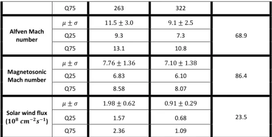
These parameters are displayed in Table 1. The last column of Table 1 presents the coverage 177
distribution, as defined in Martinez et al, (2019b), showing the percentage of common distribution for 178
a given parameter between the two dynamic pressure groups. Except for the solar wind density and 179
flux, and obviously for the dynamic pressure, all solar wind properties show similar variations with 180
about 70 %, or more, of the distribution of each of these parameters in common. In other words, the 181
EUV irradiance, IMF intensity, Alfven and magnetosonic Mach numbers, solar wind speed and MSE 182
angle are similar during these two set of measurements. The spatial coverage of the ion precipitation 183
measurements, characterized by the MSE angle and the solar zenith angle, is also similar during these 184
two set of measurements. 185
9 The presence of crustal magnetic fields (Acuña et al., 1999; Connerney et al., 2005) can influence locally 187
the precipitating ion flux, as shown by Hara et al. (2017b). In order to limit the potential influence of 188
the crustal fields (Leblanc et al. 2017; Hara et al. 2017b), we also only consider measurements 189
performed when the average magnetic field between 200 and 350 km was less than 60 nT. Moreover, 190
to further limit the potential role of the crustal fields on the precipitation, we also consider only 191
MAVEN measurements performed when the main crustal field region (centered at 180° GEO East 192
longitude and -50° GEO latitude) was in the nightside, meaning when the subsolar point has a GEO 193
longitude from -60° to 60°. 194
195
High Pdyn
[1.0,2.6] nPa
[0.3,1.0] nPa
Low Pdyn
coverage (%)
Common
EUV Flux (𝒎𝑾. 𝒎 𝟐) 𝜇 ± 𝜎 0.22 ± 0.04 0.22 ± 0.03 85.5 Q25 0.19 0.20 Q75 0.24 0.23 Dynamic pressure (𝒏𝑷𝒂) 𝜇 ± 𝜎 1.44 ± 0.41 0.63 ± 0.19 0.0 Q25 1.13 0.46 Q75 1.63 0.79 Solar Zenith Angle (°) 𝜇 ± 𝜎 96 ± 28 96 ± 28 89.7 Q25 80 77 Q75 115 118 Electric field (𝒎𝑽. 𝒎 𝟏) 𝜇 ± 𝜎 1.44 ± 0.55 1.04 ± 0.45 68.6 Q25 1.00 0.74 Q75 1.77 1.20 IMF (𝒏𝑻) 𝜇 ± 𝜎 3.90 ± 1.12 3.23 ± 0.95 69.1 Q25 2.92 2.50 Q75 4.52 3.60 Speed (𝒌𝒎. 𝒔 𝟏) 𝜇 ± 𝜎 448 ± 80 423 ± 78 80.1 Q25 376 370 Q75 495 467 Density (𝒄𝒎 𝟑) 𝜇 ± 𝜎 4.67 ± 1.93 2.25 ± 0.97 40.9 Q25 3.28 1.49 Q75 5.69 2.78 MSE angle(°) 𝜇 ± 𝜎 178 ± 110 203 ± 110 86.2 Q25 94.7 153
10 Q75 263 322 Alfven Mach number 𝜇 ± 𝜎 11.5 ± 3.0 9.1 ± 2.5 68.9 Q25 9.3 7.3 Q75 13.1 10.8 Magnetosonic Mach number 𝜇 ± 𝜎 7.76 ± 1.36 7.10 ± 1.38 86.4 Q25 6.83 6.10 Q75 8.58 8.07
Solar wind flux (𝟏𝟎𝟖 𝒄𝒎 𝟐𝒔 𝟏)
𝜇 ± 𝜎 1.98 ± 0.62 0.91 ± 0.29
23.5
Q25 1.57 0.68
Q75 2.36 1.09
Table 1: Mean µ, standard deviation , first quartile Q25 and third quartile Q75 of the solar zenith 196
angle and each solar planetary parameter distribution for the two sets of precipitating flux 197
measurement. The last column provides the percentage of the area in common between the two 198
distributions. 199
200
C. MAVEN’s ion precipitation measurements 201
In order to reconstruct the precipitating ion energy flux, we use the method developed by Leblanc et 202
al. (2015) and Martinez et al (2019a). We use MAVEN observations of the two sets of measurements 203
performed between 200 and 350 km. Within such altitude range, any ions moving toward the planet 204
in a cone of less than 75° with respect to the local nadir direction has a very large probability to impact 205
Mars’ atmosphere. Therefore, to reconstruct the precipitating flux, we sum all measurements of SWIA 206
(and STATIC) anodes with a FOV corresponding to a cone of less than 75° from the local zenith 207
direction. Moreover, in order to exclude the reconstructed precipitating flux with poor coverage, we 208
only consider measurements during which the total FOV of SWIA (and STATIC) anodes covers more 209
than 65 % of the 75° solid angle cone centered on the zenith direction. In the case of MAVEN/SWIA 210
measurements, which has a low signal-to-noise ratio at high energy, we adapted the method from 211
Martinez et al. (2019a) to remove an average background induced by Solar Energetic Particles (SEP). 212
11 Compared to MAVEN/SWIA, MAVEN/STATIC is less sensitive to SEPs because its measurements 213
technique is based on double coincidence (McFadden et al., 2015). In case of intense SEP events or 214
background level, STATIC measurements with poor quality were flagged and systematically excluded 215
from our analysis. So, the background level of MAVEN/STATIC is assumed to be negligible. 216
217
In this study, MAVEN observations obtained from June 4th, 2015 to July 20th, 2017 have been
218
categorized into two groups with similar spatial coverage: high dynamic pressure with 1.44 nPa 219
averaged on 226 ion precipitation spectra by MAVEN/SWIA, and low dynamic pressure with 0.63 nPa 220
averaged on 454 ion precipitation spectra by MAVEN/SWIA. 221
222
III. LatHyS Model 223
224
In order to simulate the Martian environment and the precipitating heavy ion flux, we choose to use 225
the hybrid approach which describes ions with a kinetic approach while the electrons are treated as a 226
fluid (Modolo et al. 2016). The hybrid model called LatHyS is a 3-D multispecies parallelized model that 227
simulates the interaction of the solar wind plasma with the neutral environment of the planet, 228
characterizing all plasma regions in the vicinity of the planet. A detailed description of the LatHyS 229
model can be found in Modolo et al. (2005 and 2016). The model uses as inputs a 3-D density 230
description of H, O and CO2 representing the thermosphere and exosphere. The neutral species
231
description is modeled from the LMD - Global Circulation Model (Forget et al, 1999; Chaufray et al. 232
2014) and the Exospheric Global Model (Yagi et al, 2012; Leblanc et al, 2017). The state of the neutral 233
environment corresponds to solar longitude Ls = 270°. The spatial resolution of the LatHyS results 234
presented in this paper is Δx = 57 km, and a mean solar activity is assumed for all the models (LatHyS, 235
EGM, LMD-GCM) and for the two solar wind dynamic pressure cases. 236
12 Simulations are set up with typical solar wind parameters based on the orbit-by-orbit average solar 238
wind parameters for the two groups of solar wind dynamic pressure, from Table 1. To facilitate the 239
interpretation of the simulated precipitation fluxes, the interplanetary magnetic field is taken with only 240
a 𝐵 component. For the period of high dynamic pressure we have: 𝑛 = 4.7 𝑐𝑚 , 𝑉 = 241
450 𝑘𝑚. 𝑠 and 𝐵 = 4.0 𝑛𝑇. For the period of low dynamic pressure we have: 𝑛 = 2.2 𝑐𝑚 , 242
𝑉 = 424 𝑘𝑚. 𝑠 and 𝐵 = 3.2 𝑛𝑇. Simulations are performed with a sub-solar longitude at 0° 243
and a subsolar latitude at -23°, meaning that the main crustal field region is located in the nightside. 244
To further analyze simulation results, for each particle we record the information of the injection 245
position, the ionization mechanism of the particle, the injection time, the precipitation time and its 246
precipitating energy. Three main sources of ions are implemented in the simulation model. A simplified 247
set of ionospheric chemistry equations is included (below 350 km) and particles created in this region 248
are labeled as ionospheric particles. Particles can also be produced by photo-ionization above 350 km, 249
where the optical depth is negligible, or undergo charge exchange reactions. Information concerning 250
the ionization processes are detailed in Modolo et al. (2016). 251
252
In this study, we consider only oxygen ions. Heavier ions (such as 𝐴𝑟 , 𝑂 and 𝐶𝑂 ) are not considered 253
because of their much lower density at high altitude according to Fox (2004) so that their contribution 254
to atmospheric sputtering should be very limited in intensity. Once a steady state of the simulation is 255
achieved, O+ ion precipitating (𝑉 < 0) below 250 km in altitude are recorded in order to construct an
256
energy flux map on a 4.5° x 4.5° longitude-by-latitude grid. To have meaningful statistics on the 257
precipitating O+ ions, the accumulation is performed over 100 solar wind proton gyro-periods (about
258
6-7 transit times of the simulation box). Each energy spectra corresponding to the impacting O+ flux is
259
computed with an energy resolution of = ~ 17 % for energy larger than 2 eV. With more than one 260
million precipitating numerical particles for each simulation, the modelled sample is large enough to 261
be statistically significant. The stationarity of the solution has been checked by comparing energy 262
13 spectra at each grid point of the map for various accumulation intervals. We found a temporal standard 263
deviation of 15-20 % indicating that the simulation converged to a stable solution. 264
265
In order to compare simulation and observation, a similar methodology to reconstruct the simulated 266
precipitation as for MAVEN measurements have been used: 267
- For each sequence of observation, the portion of MAVEN trajectory during which the 268
precipitating flux was measured (between 200 km and 350 km in altitude) is 269
reconstructed in the simulated MSE reference frame. 270
- The simulated energy spectra of the precipitating flux along each of these portions of 271
MAVEN trajectory are then reconstructed and averaged. If, for a given energy bin, the 272
simulated flux is lower than the threshold corresponding to MAVEN/SWIA background, 273
the simulated precipitated ion energy flux, for this energy bin, is not considered to 274
calculate the average. 275
276
IV. LatHyS simulated precipitation and MAVEN precipitating measurements 277
A. Comparison between MAVEN observation of the precipitating flux and LatHyS simulated 278
flux 279
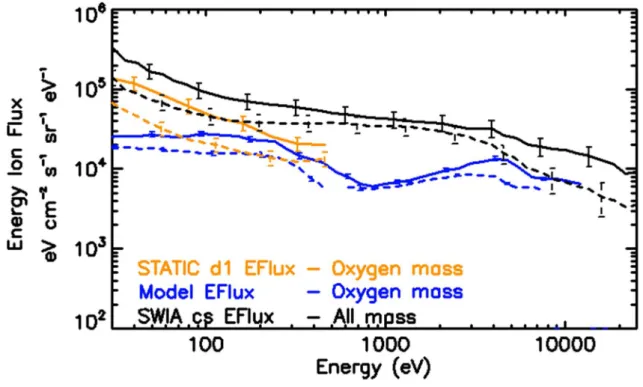
Figure 1 shows the comparison of the spectrum of the average precipitating ion energy flux for 280
MAVEN/SWIA, MAVEN/STATIC and as simulated for the two dynamic pressure cases. The energy 281
dependence of the differential flux is similar from one solar wind dynamic pressure case to the other 282
for both instruments. For both dynamic pressure cases, the low-energy component of the precipitating 283
oxygen ion energy flux measured by MAVEN/STATIC and simulated follow similar dependency with 284
higher fluxes for larger dynamic pressure. Below 50 eV, we notice an increasing discrepancy between 285
observation and simulation. This difference can be, in part, explained by the limited resolution of the 286
simulations (57 km). At low energy, the main component of the oxygen ion precipitation comes from 287
the ionospheric region (below 350 km in altitude) where the spatial resolution of the simulation 288
14 remains several times higher than the thermospheric height scale (11-20 km). Because of this, ion 289
production in the ionosphere (below 350 km in altitude) is probably poorly described, making it less 290
sensitive to any external variations. 291
For energy larger than a few keVs, as explained in section II.A, MAVEN/SWIA observed ion precipitation 292
should be in large proportion composed of O+ ions. Above 3 to 4 keV, there is a clear increase of the
293
measured and simulated precipitating fluxes from the low dynamic pressure case to the high dynamic 294
pressure case. The gap between the MAVEN/SWIA curves (all species) and those of the model (only 295
oxygen ions) between 300 eV and 3-4keV can be explained by the contribution of other species in the 296
observed ion precipitation (mainly protons, in particular around the solar wind energy, probably 297
produced in the hydrogen corona). 298
Table 2 shows the integrated precipitating ion energy flux for each dynamic pressure case and two 299
energy ranges: low energy [30-650] eV) and high energy [650-25000] eV. The ion precipitation 300
increases when the dynamic pressure of the solar wind increases, as previously observed by Hara et 301
al. (2017a) with MAVEN/SWIA and MAVEN/STATIC measurements. It increases by a factor between 302
1.7 and 2.0 at low energy and by factor 1.9 to 2.1 at high energy. Both simulation and observation 303
agree relatively well when comparing the two dynamic pressure cases, even if the simulation predicts 304
a systematic factor 4 lower integrated flux with respect to SWIA observed precipitation for both solar 305
dynamic pressure cases and energy ranges. At high energy, this factor can be partially explained by the 306
fact that the modelled precipitating ion energy flux becomes lower than the MAVEN/SWIA background 307
and so, the energy ion flux is not considerate, which slightly underestimate the modelled ion 308
precipitation. In other words, even if the simulation did not perfectly reproduce the absolute intensity 309
of the observed precipitation, the simulated variation of the precipitating flux with increasing pressure 310
might be driven by a similar mechanism to the one controlling the dependency of this flux in MAVEN 311
observations. 312
15 313
Figure 1: Average precipitating ion differential energy spectra as measured by MAVEN/SWIA 314
(black – all species), MAVEN/STATIC (orange – oxygen mass) and simulated (blue – oxygen mass) 315
during high pressure period (line) and low pressure period (dashed line). The verticals lines 316
correspond to the standard error of the average flux. 317
318
Integrated precipitating ion energy flux
Low energy [30-650] eV High energy [650-25000] eV
High pressure
period
SWIA (all species) 4.27 (±0.93)× 10 7 42.8 (±11.1)× 107 STATIC 2.06 (±0.41)× 107 Model 1.03 (±0.08)× 107 10.8 (±0.6)× 107 SWIA 2.57 (±0.58)× 107 22.4 (±7.2)× 10716
Low pressure
period
(all species) STATIC 9.89 (±1.98)× 106 Model 6.07 (±0.04)× 106 5.10 (±0.15)× 107Ratio
HPDYN/LPDYN
SWIA (all species) 1.66 1.91 STATIC 2.08 Model 1.70 2.12Table 2: Integrated precipitating ion energy flux as measured by MAVEN/STATIC (only oxygen ion) 319
and MAVEN/SWIA (all species) and modelled by LatHyS (only oxygen ion) for each period. The last 320
three line correspond to the ratio between the high pressure period values and the low pressure 321
period values for each instrument. In brackets, the 1-sigma standard deviation (uncertainty) of the 322
precipitating ion energy flux values. The integrated ion precipitation unit is in 𝑒𝑉. 𝑐𝑚 . 𝑠𝑟 . 𝑠 . 323
324
B. Origins and parameters controlling the simulated precipitating fluxes 325
Figure 2 displays the impact energy of the precipitating oxygen ions (of ionospheric origin, created by 326
photo-ionization or by charge exchange) as a function of their injection (creation) position in the (X, 𝜌) 327
coordinate system with 𝜌 = √𝑌 + 𝑍 , for the low pressure case. The negative values of 𝜌 328
correspond to the Southern Hemisphere MSE (Z < 0) while positive values indicate the Northern 329
Hemisphere (Z > 0). The lack of injected particles behind Mars is explained by the shadow of the planet, 330
preventing photo-ionizations. The precipitating ions with energy higher than the solar wind (800 eV - 331
1 keV) are formed in the southern hemisphere MSE and their final energy depends on their altitude of 332
creation (by ionization). This energy-altitude injection relation is consistent with Jarvinen et al. (2018) 333
and can be explained by the time spent by an ion in the high electric field regions (essentially the solar 334
wind and the magnetosheath). In the northern hemisphere, it can also be seen that precipitating ions 335
are mainly formed within or downstream of the pile-up magnetic region. The high-energy ions 336
17 precipitate mainly in the Southern hemisphere and on the Martian dayside (not shown) as simulated 337
in Luhmann and Kozyra (1991). This distribution of the origin position of precipitating ions and their 338
impact energy can be explained by the intensity of the electric field and its direction (Chaufray et al., 339
2007; Curry et al., 2015). In the upstream solar wind and the magnetosheath, the newly born ions will 340
be accelerated in the direction of the convective electric field. Ions formed in the northern hemisphere 341
MSE will be moved away Mars, while ions formed in the southern hemisphere MSE will be accelerated 342
toward Mars, as observed in Hara et al. (2017a). This is why for high X > 0 and 𝜌 > - 0.5 in Figure 2, 343
there are almost no precipitating ions formed upstream the bow shock. The ions formed inside the 344
magnetosheath will see a disturbed electric field direction which may lead them to precipitate. To 345
summarize, this result indicates that oxygen ions created above the ionosphere in the –E hemisphere 346
can more easily precipitate toward the planet rather than those created in the +E hemisphere, in good 347
agreement with previous numerical simulations (Chaufray et al., 2007; Fang et al., 2010; Curry et al., 348
2015). 349
18 351
Figure 2: Map of the origin position of the precipitating ions produced either in the ionosphere (below 352
350 km in altitude), by photo-ionization or by charge exchange for the low pressure period. The impact 353
energy of the modelled ions is shown in color. The black lines correspond to the ion magnetopause 354
boundary (closest to Mars) and bow shock (farthest from Mars) location. The dashed white circle 355
corresponds to the upper limit of the ionosphere (350 km in altitude). 356
19 Figure 3 displays the energy distribution of the simulated precipitating oxygen ion energy flux averaged 358
over the whole oxygen ion precipitation map (without removing the background value of 359
MAVEN/SWIA). In the high dynamic pressure case, the maximum energy of the ions impacting the 360
atmosphere reaches 14 keV whereas in the low dynamic pressure case only 10 keV. This illustrates the 361
fact that ions created at the same position see a stronger electric field intensity in the case of high 362
pressure (𝐸 = 1.44 𝑚𝑉. 𝑚 upstream of the bow shock) than in the case of the low pressure (𝐸 = 363
1.04 𝑚𝑉. 𝑚 upstream of the bow shock) 364
As a matter of fact, the main difference between the two modelled dynamic pressure cases can be 365
described as a global shift in energy, associated with a change in the local electric field intensity, and 366
an increase of the intensity of the precipitating ions. As an example, in the case of the ionospheric ions 367
(red lines in Figure 3), there is a significant increase of the precipitating flux with increasing dynamic 368
pressure above 50 eV, as observed by the MAVEN/STATIC. In the same way, in the case of the ions 369
produced by photoionization Figure 3, there is globally an increase in energy of the precipitating ions 370
due to the increase of the electric field close to Mars when increasing the dynamic pressure. 371
20 Figure 3: Simulated precipitating oxygen ion differential energy spectra. Solid line: high dynamic 373
pressure case. Dashed line: low dynamic pressure case. Red lines: oxygen ionospheric ions. Dark blue 374
lines: oxygen ions produced by charge exchange. Light blue lines: oxygen ions produced by photo-375
ionization. Black lines: total precipitating oxygen ions flux. Vertical lines: standard deviation of the flux 376
estimated by performing several snapshots during the simulation. 377
378
However, in the case of the ion produced by charge exchange, a higher dynamic pressure induces not 379
only a gain of energy of the precipitating particle but also an increase in the charge exchange ionization 380
rate between solar wind protons and O atmospheric neutral particles which should be proportional to 381
the solar wind particle flux ~ 𝑛 𝑉 . The ionization rate by charge exchange should increase by a 382
factor ~ 2.3 which is the ratio between the solar wind flux in the high dynamic pressure case to the 383
solar wind flux in the low dynamic pressure case. This ratio is very close to the ratio of the precipitating 384
fluxes of the ions produced by charge exchange between the high and low dynamic pressure cases 385
(equal to ~ 2.7). On the other hand, the production rates of ion in the ionosphere or by photo-ionization 386
are not or only in a limited way influenced by the change of the solar wind dynamic pressure. As shown 387
in Figure 3 in the case of the high dynamic pressure (dark blue line), the precipitating flux is dominated 388
by ions produced by charge exchange above 1 keV. In the low dynamic pressure case, charge exchange 389
and photo-ionization produces roughly the same amount of ions according to the simulation. 390
The main lessons from the simulation are: 391
- An increase of the dynamic pressure should lead to a global increase of the energy of 392
the ion precipitating in the atmosphere, roughly proportionally with the change of the 393
motional electric field in the undisturbed solar wind. 394
- An increase of the dynamic pressure should lead to an increase of the charge exchange 395
rate in a proportion roughly equivalent to the increase in solar wind flux. This effect 396
should be observable at high energy, above typically 1 keV, where the contribution of 397
21 the charge exchange mechanism on the production of the precipitating ion starts to 398
dominate. 399
- Below 1 keV, the precipitating ion energy flux should be dominated by the ionospheric 400
ions which are poorly described by LatHyS due to a limitation in spatial resolution. 401
We also evaluated the impact of the dynamic pressure on the plasma boundaries (essentially on the 402
bow shock position) by comparing the precipitating flux of oxygen ions produced by photo-ionization 403
upstream of the bow shock for both cases. With a small difference between the two cases, we 404
concluded that the precipitating ion flux is only weakly influenced by the compression of the bow shock 405
with increasing solar dynamic pressure (see supplementary document). 406
407
V. Summary and Conclusion 408
Solar wind observations around Mars from the MAVEN spacecraft from 04 June 2015 to 20 July 2017 409
are organized into two sets of measurements corresponding to two periods of significantly different 410
solar dynamic pressure. Beside different solar wind conditions, all other parameters that could 411
potentially influence the state of Mars’ atmosphere and magnetosphere are carefully estimated in 412
order to be equivalent in both samples (by selecting only observations with the same solar conditions 413
and geographic coverage). From these two periods, we then use MAVEN portions of orbit between 414
350 and 200 km in altitude to reconstruct the precipitating ion energy fluxes from SWIA (Halekas et al. 415
2015) and STATIC (McFadden et al. 2015) measurements following the method developed in Leblanc 416
et al. (2015) and Martinez et al. (2019a). 417
The average solar conditions of each period are then used to simulate Mars’ environment using LatHyS 418
hybrid model (Modolo et al. 2016). These two simulations are realized for the same solar extreme 419
ultra-violet conditions, the same season of the Martian atmosphere (LS = 270°), with the same 420
orientation of the Interplanetary Magnetic Field and the main crustal field placed in the nightside. A 421
22 method is also developed in order to reconstruct the oxygen ion precipitation from both simulations 422
using the same approach as when analyzing MAVEN measurements. 423
The precipitating ion energy flux measured by MAVEN/STATIC and MAVEN/SWIA increases with the 424
increase of the solar wind dynamic pressure, which is consistent with previous studies (Hara et al., 425
2017a). The increase of the dynamic pressure from 0.63 to 1.44 nPa is clearly associated with an 426
increase at the same order of the precipitating oxygen ion energy flux measured by MAVEN/STATIC 427
from 9.9 to 20.6 × 10 eV. cm . sr . s (a ratio of ~ 2.1) for the low energy range (from 30 to 650 428
eV). From 650 eV to 25000 eV, observations by MAVEN/SWIA show an increase from 22.4 to 42.8 × 429
107 eV. cm−2. sr−1. s−1 (a ratio of ~ 1.9) with a similar order as the increase in solar wind dynamic
430
pressure. 431
Such increase can be explained, according to the simulation results by several mechanisms. The 432
increase of the dynamic pressure leads to a global increase of the energy and intensity of the ion 433
precipitating into the atmosphere. In terms of energy differential precipitating flux, this is equivalent 434
to a shift in energy of the flux proportional to the increase of the solar wind convective electric field 435
intensity upstream to Mars, and an increase of the intensity of the energy differential precipitating 436
flux, proportional to the increase of the solar wind flux because an increase of the solar wind flux also 437
implies a change of the charge exchange rate between the incident solar wind ions and the planetary 438
exosphere. Such effect is particularly observable above 1 keV in the simulated precipitating ion energy 439
flux where the flux is in a large proportion composed of planetary oxygen ions formed by charge 440 exchange. 441 442 Acknowledgements 443
This work was supported by the DIM ACAV and the ESA/ESTEC faculty. This work was also supported 444
by CNES “Système Solaire” program and by the “Programme National de Planétologie” and 445
“Programme National Soleil-Terre”. This work is also part of HELIOSARES Project supported by the ANR 446
23 (ANR-09-BLAN-0223), ANR MARMITE (ANR-13-BS05-0012-02) and ANR TEMPETE (ANR-17-CE31-0016). 447
Spacecraft data used in this paper are archived and available in the Planetary Data System Archive 448
(https://pds.nasa.gov/). Numerical simulation results used in this article can be found in the simulation
449 database (http://impex.latmos.ipsl.fr). 450 451 452 References 453
Acuña, M. H., et al. (1999), Global distribution of crustal magnetization discovered by the Mars Global 454
Surveyor MAG/ER Experiment, Science, 284, 790-793, doi:10.1126/science.284.5415.790. 455
Anderson D.E and C.W. Hord, Multidimensional radiative transfer: Applications to planetary coronae, 456
Planetary and Space Science, Volume 25, Issue 6, 1977, Pages 563-571, ISSN 0032-0633, 457
https://doi.org/10.1016/0032-0633(77)90063-0.
458
Andersson, L., R. E. Ergun, and A. I. F. Stewart (2010), The Combined Atmospheric Photochemistry and 459
Ion Tracing code: reproducing the Viking Lander results and initial outflow results, Icarus, 206(1), 120– 460
129, https://doi.org/10.1016/j.icarus.2009.07.009. 461
Barabash, S., Lundin, R., Andersson, H. et al. (2006), The analyzer of space plasmas and energetic atoms 462
(ASPERA-3) for the Mars Express mission, Space. Sci. Rev., 126, 113-164, 463
https://doi.org/10.1007/s11214-006-9124-8 464
Brain, D. A., F. Bagenal, Y.-J. Ma, H. Nilsson, and G. Stenberg Wieser (2016), Atmospheric escape from 465
unmagnetized bodies, J. Geophys. Res. Planets, 121, 2364–2385, doi:10.1002/2016JE005162. 466
Chassefière, E., and F., Leblanc (2004), Mars atmospheric escape and evolution; interaction with the 467
solar wind, Planet. Space Sci., 52, 1039-1058, doi: 10.1016/j.pss.2004.07.002 468
24 Chaufray, J. Y., R. Modolo, F. Leblanc, G. Chanteur, R. E. Johnson, and J. G. Luhmann (2007), Mars solar 469
wind interaction: Formation of the Martian corona and atmospheric loss to space, J. Geophys. Res., 470
112, E09009, doi:10.1029/2007JE002915. 471
Chaufray, J.-Y., Gonzalez-Galindo, F., Forget, F., Lopez-Valverde, M., Leblanc, F., Modolo, R., Hess, S., 472
Yagi, M., Blelly, P.-L., and Witasse, O. (2014), Three-dimensional Martian ionosphere model: II. Effect 473
of transport processes due to pressure gradients, J. Geophys. Res. Planets, 119, 1614– 1636, 474
doi:10.1002/2013JE004551.
475
Chicarro, A., P. Martin, and R. Trautner (2004), The Mars Express mission: An overview, in Mars 476
Express: A European Mission to the Red Planet, Eur. Space Agency Spec. Publ., ESA SP-1240, edited by 477
A. Wilson and A. Chicarro, pp. 3–16, ESA Publ. Div., ESTEC, Noordwijk, Netherlands. 478
Connerney, J.E.P., Espley, J., Lawton, P. et al., The MAVEN Magnetic Field Investigation, Space Sci Rev 479
(2015a) 195 : 257., https://doi.org/10.1007/s11214-015-0169-4 480
Connerney, J.E.P., Espley, J.R., DiBraccio, G.A., et. al. (2015b). First results of the MAVEN magnetic field 481
investigation. Geophys. Res. Lett., 42, 8819–8827, doi:10.1002/2015GL065366. 482
Curry S. M., Luhmann J. G., and al. (2015), Response of Mars 0+ pickup ions to the 8 March 2015 ICME: 483
Inferences from MAVEN data-based models., Geophys. Res. Lett, 42, 9095-9102, 484
doi:10.1002/2015GL06304. 485
Diéval, C., et al. (2012), A case study of proton precipitation at Mars: Mars Express observations and 486
hybrid simulations, J. Geophys. Res., 117, A06222, doi:10.1029/2012JA017537. 487
Dong, Y., Fang, X., Brain, D. A., McFadden, J. P., Halekas, J. S., Connerney, J. E. P., Eparvier, F., 488
Andersson, L., Mitchell, D., and Jakosky, B. M. (2017), Seasonal variability of Martian ion escape 489
through the plume and tail from MAVEN observations, J. Geophys. Res. Space Physics, 122, 4009–4022, 490
doi:10.1002/2016JA023517. 491
25 Edberg, N., Brain, D. A., Lester, M., Cowley, S. W. H., Modolo, R., Franz, M., and Barabash S. (2009), 492
« Plasmas boundary variability at Mars as observed by Mars Global Surveyor and Mars Express », Ann. 493
Geophys., 27, 3537-3550, doi:10.5194/angeo-27-3537-2009. 494
Edberg, N. J. T., Lester, M., Cowley, S. W. H., Brain, D. A., Fränz, M., and Barabash, S. (2010), 495
Magnetosonic Mach number effect of the position of the bow shock at Mars in comparison to Venus, 496
J. Geophys. Res., 115, A07203, doi:10.1029/2009JA014998. 497
Eparvier, F.G., Chamberlin, P.C., Woods, T.N. et al., The Solar Extreme Ultraviolet Monitor for MAVEN, 498
Space Sci Rev (2015) 195 : 293., https://doi.org/10.1007/s11214-015-0195-2 499
Fang, X., Liemohn, M. W., Nagy, A. F., Luhmann, J. G., and Ma, Y. (2010), Escape probability of Martian 500
atmospheric ions: Controlling effects of the electromagnetic fields, J. Geophys. Res., 115, A04308, 501
doi:10.1029/2009JA014929.
502
Fang, X., S. W. Bougher, R. E. Johnson, J. G. Luhmann, Y. Ma, Y.-C. Wang, and M. W. Liemohn (2013), 503
The importance of pickup oxygen ion precipitation to the Mars upper atmosphere under extreme solar 504
wind conditions, Geophys. Res. Lett., 40, 1922–1927, doi:10.1002/grl.50415. 505
Forget, F., Hourdin, F., Fournier, R., Hourdin, C., Talagrand, O., Collins, M., … Huot, J.-P. (1999). 506
Improved general circulation models of the Martian atmosphere from the surface to above 80 km. 507
Journal of Geophysical Research, 104(E10), 24,155–24,175. https://doi.org/10.1029/1999JE001025 508
Fedorov A., Budnik E., Sauvaud J.-A., Mazelle C., Barabash S., Lundin R., Acuña M., Holmström M., 509
Grigoriev A., Yamauchi A., Andersson H., Thocaven J.-J., Winningham D., Frahm R., Sharber J.R., 510
Scherrer J., Coates A.J., Linder D.R., Kataria D.O., Kallio E., Koskinen H., Säles T., Riihelä P., Schmidt W., 511
Kozyra J., Luhmann J., Roelof E., Williams D., Livi S., Curtis C.C., Hsieh K.C., Sandel B.R., Grande M., 512
Carter M., McKenna-Lawler S., Orsini S., Cerulli-Irelli S., Maggi M., Wurz P., Bochsler P., Krupp N., Woch 513
J., Fränz M., Asamura K., Dierker C., Structure of the Martian wake, Icarus, Volume 182, Issue 2, 2006, 514
Pages 329-336, ISSN 0019-1035, https://doi.org/10.1016/j.icarus.2005.09.021. 515
26 Fox, J.. (2004). Response of the Martian thermosphere/ionosphere to enhanced fluxes of solar soft X 516
rays. Journal of Geophysical Research. 109. Doi:10.1029/2004JA010380. 517
Halekas, J.S., Taylor, E.R., Dalton, G. et al., The Solar Wind Ion Analyzer for MAVEN, Space Sci Rev (2015) 518
195 : 125., https://doi.org/10.1007/s11214-013-0029-z 519
Halekas, J. S., et al. (2017), Structure, dynamics, and seasonal variability of the Mars-solar wind 520
interaction: MAVEN Solar Wind Ion Analyzer in-flight performance and science results, J. Geophys. Res. 521
Space Physics, 122, 547–578, doi: 10.1002/2016JA023167. 522
Hall, B. E. S., et al. (2016), Annual variations in the Martian bow shock location as observed by the Mars 523
Express mission, J. Geophys. Res. Space Physics, 121, 11,474– 11,494, doi:10.1002/2016JA023316. 524
Hara, T., K. Seki, Y. Futaana, M. Yamauchi, M. Yagi, Y. Matsumoto, M. Tokumaru, A. Fedorov, and S. 525
Barabash (2011), Heavy-ion flux enhancement in the vicinity of the Martian Ionosphere during CIR 526
passage: Mars Express ASPERA-3 observations, Journal of Geophysical Research, vol. 116, A02309, 527
doi:10.1029/2010JA015778, 2011. 528
Hara, T., et al. (2017a), MAVEN observations on a hemispheric asymmetry of precipitating ions toward 529
the Martian upper atmosphere according to the upstream solar wind electric field, J. Geophys. Res. 530
Space Physics, 122, 1083–1101, doi: 10.1002/2016JA023348 531
Hara T. et al., (2017b), Evidence for crustal magnetic field control of ions precipitating into the upper 532
atmosphere of Mars, J. Geophys. Res. Space Physics, 122, doi: 10.1029/2017JA024798. 533
Jakosky, B.M., Lin, R.P., Grebowsky, J.M. et al., The Mars Atmosphere and Volatile Evolution (MAVEN) 534
Mission, Space Sci Rev (2015) 195 : 3. https://doi.org/10.1007/s11214-015-0139-x 535
Jarvinen, R., and Kallio, E. (2014), Energization of planetary pickup ions in the solar system, J. Geophys. 536
Res. Planets, 119, 219– 236, doi:10.1002/2013JE004534. 537
27 Jarvinen, R., Brain, D. A., Modolo, R., Fedorov, A., & Holmström, M. (2018). Oxygen ion energization at 538
Mars: Comparison of MAVEN and Mars express observations to global hybrid simulation. Journal of 539
geophysical research: Space physics, 123(2), 1678-1689. https://doi.org/10.1002/2017JA024884 540
Johnson, R.E., Plasma-induced sputtering of an atmosphere, Space Sci Rev (1994) 69: 215. 541
https://doi.org/10.1007/BF02101697 542
Johnson, R. E., D. Schnellenberger, and M. C. Wong (2000), The sputtering of an oxygen thermosphere 543
by energetic O+, J. Geophys. Res., 105(E1), 1659–1670, doi:10.1029/1999JE001058.
544
Krasnopolsky, V. A., and P. D. Feldman (2001). Detection of molecular hydrogen in the atmosphere of 545
Mars. Science, 294,1914– 1917. 546
Leblanc, F. and R.E Johnson, Sputtering of the Martian atmosphere by solar wind pick-up ions, Planet. 547
Space Sci., 49, 645-656, 2001, doi:10.1016/S0032-0633(01)00003-4. 548
Leblanc F. and R.E. Johnson (2002), Role of molecules in pick-up ion sputtering of the Martian 549
atmosphere, J. Geophys. Res., https://doi.org/10.1029/2000JE001473 550
Leblanc F., R. Modolo and al. (2015), Mars heavy ion precipitating flux as measured by Mars 551
Atmosphere and Volatile EvolutioN, Geophys. Res. Lett, 42, 9135-9141, doi: 10.1002/2015GL066170. 552
Leblanc, F., Chaufray, J. Y., Modolo, R., Leclercq, L., Curry, S., Luhmann, J., … Jakosky, B. (2017). On the 553
origins of Mars' exospheric nonthermal oxygen component as observed by MAVEN and modeled by 554
HELIOSARES. Journal of Geophysical Research: Planets, 122, 2401–2428. 555
https://doi.org/10.1002/2017JE005336 556
Lillis, R.J., Brain, D.A., Bougher, S.W. et al., Characterizing Atmospheric Escape from Mars Today and 557
Through Time, with MAVEN, Space Sci Rev (2015) 195: 357. https://doi.org/10.1007/s11214-015-0165-558
8 559
28 Lillis, R. J., et al. (2017), Photochemical escape of oxygen from Mars: First results from MAVEN in situ 560
data, J. Geophys. Res. Space Physics, 122, 3815– 3836, doi:10.1002/2016JA023525. 561
Luhmann, J. G. (1990), A model of the ion wake of Mars, Geophysical Research Letters, 17, 869– 872, 562
https://doi.org/10.1029/GL017i006p00869 563
Luhmann, J. G., and J. U. Kozyra (1991), Dayside pick-up oxygen ion precipitation at Venus and Mars: 564
Spatial distributions, energy deposition and consequences, J. Geophys. Res., 96(A4), 5457–5467, doi: 565
10.1029/90JA01753. 566
Luhmann, J. G., R. E. Johnson, M. H. G. Zhang, Evolutionary impact of sputtering of the Martian 567
atmosphere by O+ pickup ions, Geophys. Res. Lett., 19, 2151–2154, 1992.
568
https://doi.org/10.1029/92GL02485 569
Lundin, R., A. Zakharov, R. Pellinen, et al. (1990), ASPERA/ Phobos measurements of the ion outflow 570
from the Martian ionosphere, Geophysical Research Letters, 17, 873–876, 571
https://doi.org/10.1029/GL017i006p00873 572
Lundin, R., Barabash, S., Fedorov, A., Holmström, M., Nilsson, H., Sauvaud, J.-A., & Yamauchi, M. 573
(2008), Solar forcing and planetary ion escape from Mars, Geophysical Research Letters, 35, L09203, 574
doi: 10.1029/2007GL032884. 575
Martinez, A., Leblanc, F., Chaufray, J. Y., Modolo, R., Romanelli, N., Curry, S., et al (2019a). Variability 576
of precipitating ion fluxes during the September 2017 event at Mars. Journal of Geophysical Research: 577
Space Physics, 124. https://doi.org/10.1029/2018JA026123 578
Martinez, A., Leblanc, F., Chaufray, J. Y., Modolo, R., Witasse, O., Dong, Y., et al. (2019b). Influence of 579
extreme ultraviolet irradiance variations on the precipitating ion flux from MAVEN observations. 580
Geophysical Research Letters, 46. https://doi.org/10.1029/2019GL083595 581
Masunaga, K., et al. (2017), Statistical analysis of the reflection of incident O+ pickup ions at Mars:
582
MAVEN observations, J. Geophys. Res. Space Physics, 122, 4089–4101, doi:10.1002/2016JA023516. 583
29 Modolo R., G. M. Chanteur, E. Dubinin and A. P. Matthews (2005), Influence of the solar EUV flux on 584
the Martian plasma environment, Ann. Geophys., 23, 433–444, doi:10.5194/angeo-23-433-2005. 585
Modolo, R., et al. (2016), Mars-solar wind interaction: LatHyS, an improved parallel 3-D multispecies 586
hybrid model, J. Geophys. Res. Space Physics, 121, 6378–6399, doi: 10.1002/2015JA022324. 587
Ramstad, R., S. Barabash, F. Yoshifumi, and M. Holmström (2017), Solar wind- and EUV-dependent 588
models for the shapes of the Martian plasma boundaries based on Mars Express measurements, J. 589
Geophys. Res. Space Physics, 122, 7279–7290, doi:10.1002/2017JA024098. 590
Rahmati, D. E. Larson, T. E. Cravens et al., MAVEN insights into oxygen pickup ions at Mars, Geophysical 591
Research Letters, 42, 21, (8870-8876), (2015). https://doi.org/10.1002/2015GL065262 592
Romanelli, N., Modolo, R., Leblanc, F., Chaufray, J.-Y., Martinez, A., Ma, Y., et al. (2018). Responses of 593
the Martian magnetosphere to an interplanetary coronal mass ejection: MAVEN observations and 594
LatHyS results. Geophysical Research Letters, 45, 7891– 7900. https://doi.org/10.1029/2018GL077714 595
Trotignon, J. G., Mazelle C., Bertucci C., and Acuna M. H. (2006), Martian shock and magnetic pile-up 596
boundary positions and shapes determined from the Phobos 2 and Mars Global Surveyor data sets, 597
Planet. Space Sci., 54, 357-369, doi:10.1016/j.pss.2006.01.003. 598
Wang, Y.-C., J. G. Luhmann, F. Leblanc, X. Fang, R. E. Johnson, Y. Ma, W.-H. Ip, and L. Li (2014), Modeling 599
of the O+ pickup ion sputtering efficiency dependence on solar wind conditions for the Martian
600
atmosphere, J. Geophys. Res. Planets, 119, 93–108, doi: 10.1002/2013JE004413. 601
Wang, Y.-C., J. G. Luhmann, X. Fang, F. Leblanc, R. E. Johnson, Y. Ma, and W.-H. Ip (2015), Statistical 602
studies on Mars atmospheric sputtering by precipitating pickup O+: Preparation for the MAVEN
603
mission, J. Geophys. Res. Planets, 120, 34–50, doi: 10.1002/2014JE004660 604
Yagi, M., Leblanc, F., Chaufray, J. Y., Gonzalez-Galindo, F., Hess, S., & Modolo, R. (2012). Mars 605
exospheric thermal and non-thermal components: Seasonal and local variations. Icarus, 221(2), 682– 606
693. https://doi.org/10.1016/j.icarus.2012.07.022 607