A Diffuse Interface Model of Transport Limited Electrochemistry in
Two-Phase Fluid Systems with Application to Steelmaking
by David Dussault
M. S., Mechanical Engineering (2002)
Submitted to the Department of Mechanical Engineering in Partial Fulfillment of the Requirement for the Degree of
Master of Science in Mechanical Engineering at the
Massachusetts Institute of Technology
February 2002 BARKER
@ 2002 Massachusetts Institute of Technology
MASSACHUSETS INSTITUTEAll rights reserved OF TECHNOLOGY
MAR 2 5 2002
LIBRARIES
Signature of A uthor . . . .
Department of Mechanical Engineering
Jan 11, 2002
Certified by. . . . .
/7 Adam C. Powell
Assistant Professor of Materials Engineering
Abstract
Electric Field-Enhanced Smelting and Refining is a process for accelerating the rate of carbon removal from steel in a steelmaking reactor. It is proposed as an alternative or a complement to the basic oxygen process. Electrodes are inserted into the metal and slag phases. The carbon is removed from the steel to form CO gas at the anodic interface, and the Fe2+ in the slag
is removed to form Fe at the cathodic interface. The overall reaction rate is limited by the transport of Fe2+ to the cathode. To accelerate the reaction, the overall cathode mass transfer
coefficient must be increased, and to do so requires an understanding of the kinetics surrounding the cathode.
An Fe-FeO-Fe electrochemical system is used as a simplified model of the steelmaking process. In this project two mathematical models of the system are developed: the classical sharp interface model and a diffuse interface model. In the diffuse interface model, the Cahn-Hilliard Equation is extended to include fluid flow and migration of ionized species due to an electric field. The voltage field is solved for using conservation of charge. Asymptotic solutions and scaling results are derived to explain phenomena surrounding the cathode. The diffuse interface model is discretized using the finite-difference method. The resulting system of nonlinear algebraic equations are solved using a Newton-Krylov solver.
The simplified 2D Fe-FeO-Fe system does not capture all phenomena of the physical slag-metal system, but does provide a foundation for a more comprehensive model to be developed in the future. The methodology developed here for coupling transport limited electrochemistry with transport equations is fundamental in that the extension to more complex systems is limited only by the development of a free energy model and the knowledge of system properties.
Acknowledgements
First I would like to thank my advisor, Professor Adam Powell. Thanks for always taking the time to answer my questions. When I was your only student and I didn't know where to start with mostly everything in the lab, you always made time for me. Thanks for being supportive and trusting my work. When the project took a turn for the worst, you supported my decision on how we could change things. Your flexibility as an advisor sometimes made things harder for me in the short term, but helped me to be a better researcher and how to solve long term problems. You were always more concerned about my well being than the status of the project. Perhaps the most important thing that I'll take from my time with you is not to lose sight of humanity when dealing with science.
To Professor McKelliget and Dr. Gerardo Trapaga, thank you for helping me in my transition into MIT. You introduced me to Professor Powell, and then backed off. Things could have been allot harder for me. You let me pretty much drop the project that we were working on, so I could focus on my studies at MIT. I probably couldn't have gotten through my first semester here without your help.
Raymundo, thanks for your help with thermodynamics. You're a good teacher. I think we complimented each other well. To my lab mates Robert and Bo, thanks for your help with Materials Science and your help with the computers. You guys were my best resources. Chris, we got through are classes together. The study sessions were great. Thanks for the talks too. Professor Sonin, thanks for agreeing to be my ME reader. Gloria, you could read me like a book. Thanks for helping me through some tough times.
To my family and friends, thanks for giving me space so I could focus at school. You let me slip into my own world at school for weeks at a time. I think that I had to do that to get through things here. Then I'd have some time off and everything would be cool again. I couldn't be around physically or mentally all the time, and you never held it against me. Thanks.
Contents
1 Introduction 10
1.1 Introductory Remarks . . . 10
1.2 Modeling and Simulation . . . . 10
1.3 Current Steelmaking Method . . . . 11
1.4 Proposed Changes ... .. ... 13
1.5 Overview of Thesis . . . . 14
2 Sharp Interface Model 17 2.1 Introductory Remarks . . . . 17 2.2 Governing Equations . . . . 17 2.3 Interface Conditions . . . . 20 2.4 Electrochemistry . . . . 23 2.4.1 Thermodynamics . . . 24 2.4.2 K inetics . . . 25
2.4.3 Charge Buildup Layer . . . . 32
2.5 Scaling and Asymptotic Solutions . . . . 34
2.5.1 1D Electrochemical System . . . . 34
2.5.2 Charge Buildup Layer . . . 36
2.5.3 Diffusion Limited Growth . . . 38
2.5.5 Buoyancy Instability . . . . 39
3 Diffuse Interface Model 41 3.1 Cahn-Hilliard . . . 41 3.2 Fe-FeO System . . . 47 3.2.1 Cahn-Hilliard . . . 47 3.2.2 Governing Equations . . . 49 4 Numerical Methods 57 4.1 Introductory Remarks . . . . 57
4.2 Discretization of Governing Equations, Finite Difference Method . . . 58
4.3 Symmetry Boundary Conditions, Shadow Nodes . . . 64
4.4 Nonlinear Solver, Multidimensional Newton's Method . . . 67
4.5 Krylov Subspace Linear Solver . . . 69
4.5.1 QR Factorization, Gram-Schmidt Algorithm . . . 69
4.5.2 General Minimization Algorithm . . . 72
4.5.3 Krylov Subspace Generation . . . 75
4.5.4 The Generalized Conjugate Residual Algorithm . . . . 77
4.6 Newton-Krylov Matrix Free Approximation . . . 78
4.7 P E T Sc . . . 79
5 Numerical Simulation Case Studies 83 5.1 Introductory Remarks . . . 83
5.2 D iffusion . . . 84
5.3 Diffusion, Migration . . . 88
5.4 Diffusion, Surface Tension Driven Convection . . . 106
6 Discussion
6.1 Introductory Remarks . . . .
6.2 Assumptions and Limitations 6.3 Applications . . . . 6.4 Future Work. . . . . 117 . . . 117 . . . 117 . . . 119 . . . 120 7 Conclusions 122 8 Appendix 124 8.1 Properties . . . 124 8.2 ComputerProgram . . . .. . . . .124
List of Figures
1.1 Slag/metal system . . . . 1 2 1.2 Slag/metal system with electrodes . .
2.1 Slag/metal Interface . . . . 2.2 Concentration profile in slag . . . . . 2.3 Transfer coefficient and free energy . 2.4 Current vs. overpotential . . . . 2.5 Current vs. overpotential for different 2.6 Initial voltage profile, 1D system. 2.7 Final voltage profile, 1D system .
2 .8 . . . .
2.9 Distorted slag/metal interface . .
2.10 Capillary instability . . . .
3.1 3.2 3.3
exchange currents
Free energy density vs. concentration Inhomogeneous system . . . . Free energy hump . . . .
3.4 Free energy of Fe-FeO system using sublattice i
4.1 4.2
. . . .
. . . . . . . .
onic liquid model .
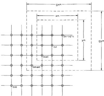
Finite difference grid . . . .
13 21 26 27 31 31 32 33 35 38 39 42 43 44 48 58 59
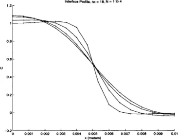
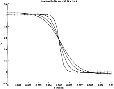
4.4 ID Newton's method 4.5 4.6 73 . . . . 80 1D minimization ... ... PETSc distributed array ... Initial concentration profile . . . . C at steady state, ID system, 16 nodes . . . . C at steady state, 1D system, 32 nodes . . . . C at steady state, ID system, 64 nodes . . . . C at steady state, 1D system, 128 nodes . . . Evolution of concentration profile, ID system, C at t=O, multi-interface system . . . . C at steady state, multi-interface system, N=1l C at steady state, multi-interface system, N=-2 C at steady state, multi-interface system, N=3 C at t=0, applied voltage . . . . C at t=1300s, applied voltage . . . . Voltage at t=1300s, applied voltage . . . . C at t=0, perturbed cathodic interface . . . . C at t=O, perturbed anodic interface . . . . . C at t=1660s, perturbed cathodic interface . . C at t=1660s, perturbed anodic interface . . . 5.1 5.2 5.3 5.4 5.5 5.6 5.7 5.8 5.9 5.10 5.11 5.12 5.13 5.14 5.15 5.16 5.17 5.18 5.19 5.20 5.21 5.22 5.23 nodes . . . 8 4 . . . 8 5 . . . 8 6 . . . 8 6 . . . 8 7 . . . 8 7 . . . . 8 9 . . . 9 0 . . . 9 1 . . . . 9 2 . . . 94 . . . 96 . . . 97 . . . 99 . . . 100 . . . 101 . . . 102 applied voltage . . . 103 )plied voltage . . . 104
C at steady state, perturbed cathodic or anodic interface, no applied voltage C at t=0, 2D drop . . . . Radius (m) 445deg vs time (sec) . . . . C at steady state, 2D drop . . . . . . . 105
. . . 109
. . . 110
111 32 C at t=1660s, perturbed cathodic interface, no C at t=1660s, perturbed anodic interface, no a . . . . 67
Chapter 1
Introduction
1.1
Introductory Remarks
The objective of this thesis is to develop a mathematical model which describes two-phase fluid/fluid systems with transport limited electrochemical reactions. There are many appli-cations for the model. The application described in this paper is a new method for low carbon steel refining known as the electric field enhanced smelting and refining of steel. In this section, relevant previous modeling methods are given, and the extension of the current modeling meth-ods to the system of interest is outlined. Following that is a description of the physical system along with a brief background to steelmaking. Finally, an overview of the entire thesis is given.
1.2
Modeling and Simulation
The model developed in this thesis is for a two phase isothermal liquid/liquid system undergoing transport limited electrochemical reactions. In order to avoid interface tracking and interface boundary conditions, a diffuse interface phase-field model was used. In the phase-field method, a composition field variable C(x, y, z) varies from 0 in one phase to 1 in the other phase. The interface spans a finite region and is represented by fractions of C.
diffusion equation originally applied to spinoidal decomposition [16]. The Cahn-Hilliard equation was extended to fluid/fluid systems by Jacqmin [9, 10] by using a modified stress tensor to account for surface tension. A general phase-field model for non-isothermal binary fluid/solid systems was developed by Sekerka and others in [18]. Papers on phase-field application and theory include [19, 20, 21, 22]. For a rigorous comparison of diffuse interface and sharp interface descriptions of fluid systems including heat transfer see Anderson and McFadden [15]. The Cahn-Hilliard free energy formulation was extended to general multi-component systems by Hoyt [17]. Multi-phase, multi-component systems are an area of active research.
In this thesis, the diffuse interface model developed by Jacqmin for two phase, two component, liquid/liquid, isothermal, flow is extended to include transport limited electrochemical reactions. To couple the transport of chemical species with electrochemistry, a migration term was added to the diffusion of chemical species equation. The Cahn-Hilliard free energy model allowed for inter-phase diffusion. Because the electrochemistry is in the transport limited region, the constitutive exponential current-voltage relations reduce to linear current-mass flux relations which reduces coupling in the governing equations. The voltage field is solved for using conservation of charge. Assuming rapid charge redistribution, the conservation of charge equation reduces to an equation for zero divergence of current flux and implicitly allows for nonuniform charge density.
1.3
Current Steelmaking Method
Steel is an iron alloy consisting of approximately 95 to 99 wt% iron, 0.01 to 2 wt% carbon, and traces of other elements such as magnesium, phosphorus, sulfur, silicon, nickel, and chromium. The amount of carbon has a direct influence on the mechanical properties of the steel such as yield strength and ductility. In general as the percentage of carbon decreases, yield strength decreases and ductility increases. For example, steel used for tools is 1.35 wt% carbon and steel used for construction is 0.25 wt% carbon. The process by which steel is derived from iron ore
Figure 1.1: Slag/metal system
steel, the steel is further processed in what is called vacuum degassing.
In the blast furnace iron ore enters along with lime (CaO), coke (refined coal) and hot air. The products react over a range of 200 to 2000 degrees C. The exiting products include hot gases such as CO and C02, molten iron, and molten slag (a mixture of oxide impurities left over from the iron ores). The density of slag is on the order of 1/2 that of steel. Thus, the slag and steel separate mechanically. The resulting slag is discarded, while the resulting iron, referred to as pig iron, is on the order of 5 wt% carbon.
The slag/melt system is shown in Figure 1.1. In the basic oxygen process a jet of oxygen is applied to the slag layer. The speed of the oxygen gas is such that the slag gets pushed aside and the gas reaches the iron melt where it combines with carbon to form carbon monoxide.
02(gas) + 2C(metal) -+ 2CO(bubble) (1.1)
However, the oxygen also reacts with the iron in the melt to form iron oxide.
02(gas) + 2Fe(metal) -+ 2FeO(slag) (1.2)
The loss of iron from the melt to the slag is an inefficiency inherent to this method. The presence of FeO in the slag leads to slag foaming and corrosion of cylinder walls, and the increase in slag mass leads to environmental issues. Discarded slag contains typically 20 to 25 wt% iron. The
Figure 1.2: Slag/metal system with electrodes
resulting steel is on the order of 0.1 wt% carbon.
In the vacuum degassing stage, the carbon content is reduced further. In this stage a vacuum is pulled over the slag-steel system. Because there is a low partial pressure of CO there is a thermodynamic driving force for CO bubbles to form and escape (along with traces of all other elements in the system). The system is not heated during the vacuum stage. Instead, the system temperature is elevated before the vacuum is applied such that the steel remains molten during the process. The resulting steel is on the order of 0.01 wt% carbon. The inefficiencies associated with this step are the energy associated with elevating the steel temperature, the energy associated with maintaining the vacuum, and the impurity of the CO removed . The carbon and oxygen must diffuse through a concentration boundary layer to reach the interface before forming CO. Thus, the process is limited by a diffusion time-scale.
1.4
Proposed Changes
A new process for refining steel known as 'Electric Field-Enhanced Refining of Steel' was devel-oped by Professor Uday Pal of Boston University [131. The idea behind this system is to generate CO from the oxygen already in the slag. The proposed system is shown in Figure 1.2. There is no external supply of oxygen. An external circuit is added to the system. The cathode lies in the slag phase, while the anode lies in the melt. Because iron is a good electrical conductor, the
and the slag/anode interface. With this configuration there is a thermodynamic driving force for electrochemical reactions to occur that are consistent with the current through the circuit. Electrons flow from the anode to the cathode. At the cathodic interface Fe is formed on the electrode.
Fe2+(slag) + 2e-
- Fe(melt) (1.3)
At the anodic interface CO is formed.
02-(slag) + C(melt) -+ CO(gas) + 2e- (1.4)
Thus, CO is formed without an external supply. The inefficiencies described above are not present in this process. The Fe that is formed on the cathode falls back into the melt (the mechanics are described in Chapter 2). Therefore, Fe is recovered from the slag instead of being lost to the slag, and there is a decrease in slag mass instead of an increase in slag mass.
The current savings associated with this process are as follows. The decrease of 20 wt% FeO in slag translates roughly into a savings of 179 MJ per metric ton of steel or $2.33 per metric ton of steel. There are 800 million tons of steel produced per year. Therefore, the total savings would be 143 * 10"J per year or $1.8 billion per year.
1.5
Overview of Thesis
The physical electrochemical slag/metal system described above is represented throughout the thesis by a simplified Fe-FeO electrochemical system. Both systems are referred to throughout the thesis. However, the chapters intentionally display a great deal of independence. The model developed here builds on previous works, but still does not capture all phenomena associated with typical applications. The independence is designed to benefit to the development of future work.
electrochemical systems. The conservation equations are given without simplifications. Interface conditions are derived based on conservation principles. Assuming that the reader is familiar with thermodynamics, an introduction to electrochemisty is given. Constitutive current-voltage relations are derived and the transport limited case is shown as an asymptotic limit. Finally, for the physical slag/metal system, the governing equations are solved for a number of simplified asymptotic cases giving rise to system length, time, and velocity scales.
Chapter 3 introduces the diffuse interface model for a two component liquid/liquid system and applies it to the Fe-FeO system. The Cahn-Hilliard equation is derived, and the coefficients are related to system properties. The phase-field model is derived by scaling parameters in the Cahn-Hilliard equation while retaining the system's surface tension. The diffuse interface governing equations are first presented in general and then are applied to the Fe-FeO system. Voltage is solved using conservation of charge. Given that the system is transport limited and that there is rapid charge redistribution, a number of terms in the conservation of charge equation are neglected and the coupling of the equations is significantly reduced.
The resulting system of equations are solved numerically. Chapter 4 describes in detail the nu-merical methods used. The finite difference method was used for space and the Crank-Nicholson scheme was used for time. Shadow nodes were used for symmetry boundary conditions. Once discretized, the system of partial differential equations becomes a system of nonlinear algebraic equations. Newton's method was used for the nonlinear solver and the generalized conjugate residual algorithm was used for the linear solver. Together they are commonly referred to as a Newton-Krylov solver. The solver allows for a finite-difference approximation to the Jacobian matrix. PETSc (The Portable, Extensible Toolkit for Scientific Computing), a collection of C libraries, was used for managing data storage and for parallel processing.
Chapter 5 contains numerical simulations of case studies. Each case study is designed to cap-ture a single phenomenon associated with physical system. The first simulation demonstrates interface diffusion and the effect that interface scaling has on the output. The second
simula-displayed along with the growth of interface perturbations. The third simulation demonstrates two phase surface tension driven convection by looking at an oscillating 2D drop. And the fourth simulation demonstrates two phase surface tension driven convection in the presence of a gravitational field. The same 2D drop is used, and the interface profile agrees with analytical calculations.
Chapter 6 and Chapter 7 are the discussion and conclusion respectively. The key assumptions are revisited. Limitations of the model are discussed. The application of the model to other physical systems is briefly described. Future development of the model to broaden the range of application is discussed. Simulation results are summarized.
Chapter 2
Sharp Interface Model
2.1
Introductory Remarks
The slag/steel system is represented here by a two-phase fluid continuum. There are two ways of modeling the system, the sharp interface model (given in this chapter) and the diffuse interface model (given in Chapter 4). In the sharp interface model the governing equations are applied to each separate phase, and boundary conditions are set at the internal interfaces. In the diffuse interface model the governing equations are applied to all phases at once, so boundary conditions are not needed at the internal interfaces. Of course, for both methods boundary conditions must be set on the outer surfaces.
This Chapter follows the sharp interface model. First, the governing equations are given for as general a case as possible. For this reason some modeling which is problem dependent is left out. Next, a number of instabilities associated with the slag/metal system are described and asymptotic solutions are derived.
1. u, x-component of velocity
2. v, y-component of velocity
3. p, pressure
4. wi, mass fraction of species i
5. q, voltage
6. pf, free charge density (free charge per unit volume of fluid) (this parameter is introduced below)
Six governing equations are needed. The fluid has a density p, a viscosity '0, and a velocity
.
In general there will be a gravitational field characterized by the gravitational acceleration-?. The first equation is conservation of x-direction momentum.a(pu) + e (pVu) =
at Dx + (nV ) + pg (2.1)
+ax-
n eVThe second equation is conservation of y-direction momentum.
(p) + V 0 (PV) = -p + (,qvv) + Pgy (2.2)
Dy
S(V)
-2D
a~.V
The first two viscous stress terms in the above two equations follow the familiar diffusion form and for a fluid with constant properties are the only remaining viscous terms. The other viscous stress terms are due to variable viscosity and incompressibility. The third equation is conservation
+ + (pr) = 0 (2.3)
at0
The fourth equation is conservation of species.
at(PW) + V
(prwi)
=M- .(3
)
(2.4)There is no generation of species in this formulation. The reactions occur at the slag/metal interface and are introduced through boundary conditions. 7 is the mass flux of species i (units are '9 ), where the flux is measured relative to the bulk velocity (diffusion flux). The molar flux of species i I (units are 'l"") is given by [1]
=-D. -zF Diciv# (2.5)
The first term represents diffusion due to concentration gradients, and the second term represents diffusion due to the effect of an electric field on an ionic component. Here Di is the diffusion coefficient of species i (units are a), zi is the charge of species i (units are mole of excess protons per mole of species i, for example, ZFe2+ = 2 and Z02- = -2), F is Faraday's constant
(F = 96485 m , where mole corresponds to mole of excess proton), R is the molar gas constant
(R = 8.314 ), and T is absolute temperature (T = 1900K). Mass flux is related to molar flux through the molar mass Mi (units are mass of i per mole of i).
i = Mi (2.6)
Therefore, the conservation of species equation becomes
a
(poW)
+ V (pwi) = MiV 0 Djf + + Dicivo# (2.7)The fifth equation is Gauss's Law inside matter, which introduces pf defined above.
v e 7 = p, (2.8)
1 is called the electric displacement, and for a linear media it is related to the electric field through
(2.9)
where e is the permittivity of the media (units are N*2). Combining gives
S
6
-
pfThe sixth and last governing equation is conservation of charge.
Dp
c
Dt
The substantial derivative is used to adjust for the transport of charge due to convection. Jc is the flux of charge (units are ) The charge flux J, is related to the molar flux
7i
throughJc = E J ziF
Combining gives
where ji is given by Equation 2.5.
2.3
Interface Conditions
Dpf-Dt
First, the velocity interface condition is derived by a mass balance at the interface.
(2.12)
(2.13)
Consider the slag/metal system shown in Figure 2.1. The interface moves with a velocity The (2.10)
(2.11)
skag
dh
MetaU
conttro(
Area=DettaA volume
Figure 2.1: Slag/metal Interface
unit vector normal to the interface is given by 7, where -# is positive when pointing in the slag direction. A infinitesimal cylindrical control volume of height dh and cross-sectional area AA encloses a small portion of the interface. The control volume moves with the interface, so mass enters on the slag side and mass leaves on the metal side (according to this positive sign convention). Applying conservation of mass gives
P8iag (Vint - Vstag) # = Pmetal (Vint - Vmetal) # (2.14)
Or, in terms of the normal components of the vectors
Pslag (Vint,n - Vsiag,n) = Pmetal (Vint,n - Vmetal,n) (2.15)
The tangential velocity is given by the no-slip condition.
The normal component of the interface velocity is found by applying conservation of electrons at the interface. The interface moving through a distance dx during a time dt. A number of electrons Ne- enter the control volume from the metal, and a number of Fe2+ atoms NFe2+ enter the control volume from the slag. They are related by
Ne- = 2NFe2+ = 2 ldx+ A (2.17)
V ol
Dividing through by dt and rearranging gives
_JVs
Vint,n = 2F (2.18)
where V, is the molar volume of slag (units are volume of slag per mole of Fe), and J is the current density (units are C
/
unit area/
unit time ). There will be a discontinuity in pressure across the interface due to surface tension. The relation isAP = o + (2.19)
(R1 R2)
Where a is the surface tension and R1 and R2 are the principal radii of curvature. The last
interface condition involves pf and
#.
Writing Gauss's law in integral form* tdA = Qf,enclosed (2.20)
where
Qf,enciosed
is the total charge enclosed in the control volume shown in FIGURE. Simplifying givesDn,siag - Dn,metal = Uf (2.21)
where of is the surface free charge density on the interface (units are charge
/
unit area). Continuing, there will be a discontinuity in the D field and a corresponding discontinuity in the E field which would imply a discontinuous gradient on voltage. However the voltage iscontinuous across the interface. That is,
0 1ag = qmetaj (2.22)
2.4
Electrochemistry
Electrochemistry is the science of chemical reactions involving electron transfer at an interface. A general electrochemical reaction has the form
O + ne = R (2.23)
where n is called the electron transfer number. The reaction occurs at an electrode/electrolyte interface. The electrode is an electrical conductor, and the electrolyte is an ionic conductor. The electrode at which reduction (reduction in oxidation number) takes place is called the cathode, and the electrode at which oxidation (increase in oxidation number) takes place is called the anode. Referring to the slag/metal system described in Section 1.4, Fe2+ is reduced to form Fe on the cathode
Fe2+(slag) + 2e- -+ Fe(melt) (2.24)
and 02- is oxidized to form CO at the anode.
02
-(slag) + C(melt) -+ CO(gas) + 2e- (2.25)
The overall chemical reaction of the system is
2.4.1
Thermodynamics
In this section energy principles are applied to electrochemical systems in equilibrium. The resulting equation known as the Nernst equation relates the cell voltage to the concentrations of each species.
Consider the general chemical reaction
aA + bB --+ cC + dD (2.27)
The free energy change associated with this reaction is
AG = AG+ RTIn aba
(A aB)
(2.28)
The free energy is also equal to the work done on the electrons as they pass through the circuit.
AG = -W,e, = -nFe (2.29)
where F is Faraday's constant, and e is the circuit voltage (cell emf). Inserting Equation 2.29 into Equation 2.28 gives Nernst Equation.
o RT aa
n F aaB
(2.30)
where e0 is the standard potential of the reaction. Considering a non-ideal solution
6 RT nF (a AB-b RT ([C]c[D] nF ([Ala[B]b) (2.31)
0,
RT In [C[D] nF n[A]a[B]bJwhere 30' is called the formal potential. For the general electrochemical reaction,
Eeq = E R In (q) (2.32)
nF C 1
2.4.2 Kinetics
In this section constitutive equations are given which describe electrochemical systems that are not in equilibrium. The resulting equation relates the current through the circuit to the applied voltage and the concentrations of each species.
Consider the general electrochemical reaction
0 + ne # R (2.33)
The arrows are used to emphasize the idea that the system is not in equilibrium. Instead forward and backward reactions are considered to be happening simultaneously.
vf = kfCo (2.34)
Vb = kbCR (2.35)
Vf and Vb are the reaction rates in the forward and backward direction (units are M), kf and kb are rate constants (units are ,), and Co and Ca are the the concentrations of each species at the interface. The net reaction rate is given by
Vnet = Vf - Vb = kfCO - kbCR (2-36)
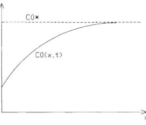
C0(xt)
Figure 2.2: Concentration profile in slag
The reaction rate at equilibrium is called the exchange velocity vo.
(2.38) vo = kfCO = kbCR
The reaction rate is related to current by using Faraday's Law.
l dN I d
(Q
)A dt Adt nF} i
nFA (2.39)
Consider the one dimensional profile shown in Figure 2.2. The rate of forward reaction is given by
Vf = kfCo (x = 0,t) = icathodic
nFA (2.40)
and the rate of backward reaction is given by
vf = kbCR(x =Ot) = Zanodic
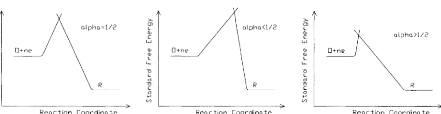
olpha=I/2 opphah/2 cnhal/
C C C c~h~/
D+ne W +ne D+ne
F r Qj Td L L -a~ d d 05 ka = kx R 7 R £ C
Reaction) Coordinate Reaction Coordinate Reaction Coordinate
Figure 2.3: Transfer coefficient and free energy
The rate constants are related to the voltage by
0 anFe
kf = kexp (- f 4e) (2.42)
kb = k exp ((1 - C) (2.43)
b ~RT)
where ko and ko are the rate constants at e = 0 for the voltage scale in use, and a, the transfer coefficient, is a measure of asymmetry of the activation barrier of the free energy curve of the reaction. The effect of a is shown qualitatively in Figure 2.3. If the system is in equilibrium and the solution is such that C = C, then the Nernst Equation gives e = 6''. Under these conditions 2.37 becomes
kC_7 = kbCR' - k = kb (2.44)
Using Equations 2.42 and 2.43
exp koep - RTO =nFE ko exp (1- a) ' k (2.45)
RT
where ko is called the standard rate constant. Therefore, ko = kf (6o') = kb (Eo'). Inserting the above equation into Equations 2.42 and 2.43 gives
kb = k exp (1 - a) R(e-eO)) (2.47)
The positive sign convention for the net current is the cathodic direction.
i = icathodic - ianodic (2.48)
Using Equations 2.40 and 2.41
i = nFAkf Co (x = 0, t) - nFAkbCR (X = 0, t) (2.49)
Using Equations 2.46 and 2.47 gives the complete current voltage characteristic of the electrode.
i = nFAk0C0 (x = Ot) exp (-a (e-o' (2.50)
-nFAkCR (x = 0, t) exp ((1 - a) I(e - ,'
At equilibrium the current-voltage relation should reduce to the Nernst Equation. At equilibrium,
i = 0, CR (0, t) = C*, and Co (0, t) = C . The equation reduces to
C* exp (- cr2
(eeq
- e')) = C* exp ((1 - a)(eeq
(E - '(2.51)=> exp
(jF
-0 - = (2.52)which is an exponential form of the Nernst Equation. Therefore, as the system approaches equilibrium the kinetic model agrees with the laws of thermodynamics.
Now, the current-voltage relation will be written in terms of exchange current and overpo-tential. The exchange current io is defined as the magnitude of the cathodic or anodic current at equilibrium.
Raising equation 2.51 to the power -a and combining with the above equation gives the final equation for exchange current.
io = nFAkOCg'-")Ci (2.54)
Overpotential 7 is defined by
= - 6 eq (2.55)
Dividing equation 2.51 by equation 2.54 gives
i - = CO (x= 0,t) Cb* -t exp -anF e-eO'
o,
(2.56)
i0 Cb C RT
CR (X = 0,t) C ~ nF ct
C* hep 1a RT
Using equation 2.52 gives the final equation.
i -Co (x = Ot) / ( anF,, CR (X = 0, t) ex (1a nFq \257
exp( T Z Ci exp (1 -a) Rr(2.57)
Now, the current-voltage relation will be written in terms of limiting current. Limiting current is the current associated with a mass transfer limited reaction. Here migration effects are excluded, and steady state is assumed. Referring to Figure 2.2, the flux of 0 to the interface in terms of the mass transfer coefficient mo is
vmt = mo (C; - Co (x = 0)) (2.58)
Using equation 2.40
= mO (C - Co (x = 0)) (2.59)
the cathodic current of a mass transfer limited reaction is given by
ihmiting,cathodic = i,c = nFAmOC (2.60)
Combining equations 2.59 and 2.60 gives an expression for for surface concentration
Co (x = 0) (2.61)
Similarly, for the anodic current
= -- MR (CR - CR (X = 0)) (2.62)
nFA
itimiting,anodic = ii,a= -nFAmRCR (2.63)
CR (X=0) i 2.4
CR 1i,a
Using equations 2.60 and 2.64, the current-overpotential equation becomes
- = - exp -_ - - -- ) exp ((1 - a) n
)
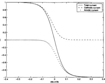
(2.65) ZO ic RT kia RT Solving for i exp (-F q) - exp ((1 - a) 26) i_ =TR (2.66) -exp ((1 - a) nFThis equation is plotted in Figures 2.4 and 2.5.
In Figure 2.4 , , and - are plotted vs 77 for si,c =-il,a = it, a = 1, n = 1, T = 298K,
and a = 0.5. The solid curve is the total current, the dashed curve is the cathodic current, and the dotted curve is the anodic current. At large positive overpotential the cathodic current is negligible, and at large negative overpotential the anodic current is negligible. Near equilibrium at 7 = 0, the cathodic and anodic contributions are the same order of magnitude. As |9q increases the system is moved further from equilibrium, and the current increases until it is limited by
-0.3 -0.2 -0.1 0 etavolts
0.1 0.2 0.3 0.4
Figure 2.4: Current vs. overpotential
-0.3 -0.2 -0.1 0 etavolts
0.1 0.2 0.3 0.4
Figure 2.5: Current vs. overpotential for different exchange currents
0.8 0.6 0.4 0.2 -0.2 -0.4 -0.6- -0.8--1 -0. - Total current - Cathodic current - Anodic current .-7 - i~'it=10 -.... - ~it=0.1'~'il=1 - 0/11=0.01 0 0.8 016 -0.4 -0.2 -S 0 -0.2 - -0.4- -0.6--0.8 1 --0.4 I ami' I 4
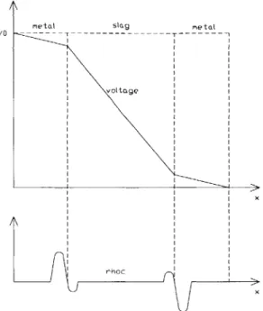
rmetol SIQ9 rmptak
votge
rhoc=O
Figure 2.6: Initial voltage profile, ID system
mass transfer. In Figure 2.5, j is plotted vs. 17 for various values of A. As Q increases for a fixed ,q the current increases. Or, as A decreases a larger q is required to reach the limiting current.
2.4.3
Charge Buildup Layer
During the initial stages of an experiment there is an inhomogeneous distribution of current and charge is seen to build up near the interface in a very thin region on the order of 10- 0m. To explain the formation of net charge buildup at the interfaces, consider the metal-slag-metal electrochemical system shown in Figure 2.6. For simplicity, there is no flow, mass transfer is by migration only, and the system has a uniform permittivity E. The governing equations are conservation of charge
Pc
a
(=
o
(2.67)
Ot Ox Ox]
and Gauss's Law
0= 2 + - (2.68)
Ox
2 6At t = 0, a voltage is applied to the system. The system initially has homogeneous charge neutrality. At small times pc = 0, and according to equation 2.68 there will be a linear voltage
Mt1Stag MetaL
vA t
Figure 2.7: Final voltage profile, 1D system
profile. The flux of charge is given by
Je
(W
=
0-
(
a)
(2.69)In general omtt>> (781ag,7 so at small times Jc,metal > > Jcsa.Charge (or a deficiency of electrons) will accumulate at the first interface, and there will be a net loss of charge at the second interface. The local charge densities will produce local electric fields which at the first interface lead to a decrease in the rate of incoming charge and an increase in the rate of the exiting charge and at the second electrode lead to an increase the rate of incoming charge and a decrease in the rate of exiting charge. A the same time, electrostatic forces act to bring negative charge to the slag side of the first interface and positive charge to the slag side of the second interface. At steady state Jc,metal = Jc,,Iag, SO 2 will be nonuniform. The final profiles are shown
2.5
Scaling and Asymptotic Solutions
It has been experimentally shown that when iron is reduced on the cathode, it does not grow out in an orderly fashion. Instead it grows out and forms liquid dendrites or fingers. The fingers are approximately cylindrical with a length of 1-4 mm and a diameter of 1/4 mm. The iron fingers are then shown to break off and fall back into the melt. In this section simple analytical results are derived which explain this phenomena.
2.5.1
1D Electrochemical System
To first gain some insight into the cathode dynamics consider a ID metal/slag electrochemical system with constant properties under a constant external electric field -40. Here, conservation of species is applied to Fe2+ only, so subscripts are excluded. Referring to Equation 2.5, the
total molar flux (diffusion plus convection) of species is given by
-Dv - zF Dcvo + cu (2.70)
RT
There is no bulk fluid motion in the slag or the metal. The speed of the interface in the positive x-direction is given by U, see Figure2.8. Therefore, relative to a coordinate system moving with the interface, the total molar flux becomes
-Dvc - zF Dc# - cU (2.71)
RT
An additional simplification is that relative to the moving interface, the system is in a steady-state. Conservation of species gives
d2C ziF d$ dc d2c dc
.g. -U
VIn=0
Figure 2.8:
where A is a constant. The boundary conditions are
c(x = 0) = 0
c (x -+ oo)
-The solution is given by
c (x)( Cbulk
- e-A )
which gives a diffusion length scale of
1 Ldif ~
The interface velocity is given by Equation 2.18
Jv,
U=-- (0.5- 2) 2(14)
~(5m 3.9 * 10 _4 mm 2F 2 (96485 mote Cbulk (2.73) (2.74) (2.75) (2.76) StUton-y C-odinat. Syst-r M-vIng C-odnet. Syst..ea sA0, -=0
A closer look at A shows that it can be decomposed into a term due to the electric field and a term due to the diffusion limited growth of the interface.
zF d4 U A= do + (2.77) RT dx D zF do 2 (964852v AEfield = zF 2 1 2.4mm' (2.78) RT dx (8.314 *K) (1900K) U (3.9 * 10-4mm) Agwth= ~ -( 1-6 ~- 3.9mm~1 (2.79)
The effects are shown to be of the same order of magnitude. Finally, the diffusion length scale
1 1
Ldiff ~ - ~ ~ 0.16mm (2.80)
A 3.9mm-1 + 2.4mm-1
2.5.2
Charge Buildup Layer
In this section a somewhat quantitative explanation of the charge buildup layer is given using simplified governing equations and scaling arguments. For a more rigorous explanation see the Gouy-Chapman model [1].
For simplicity, consider a liquid Fe-FeO system with no flow, with mass transfer by migration only, and with a uniform permittivity E. The governing equations are conservation of charge
=Pc
a
(o
(2.81)at Ox ax~
and Gauss's Law
0 = + - (2.82)
Ox
2 cterms in Gauss's law are the same order of magnitude.
(920
Solving for L gives
Pc
AO
PcPc
Using the bulk concentration of Fe in FeO, c* ', as an estimate for charge density, the open circuit
voltage as an estimate for the voltage difference, and the e co
(0.2V) (8.854 * (4.983* 104)
(
10-12 2)
2) (96485 C)
The time scale for the charge buildup layer to form is given by r. As the charge buildup layer is forming the terms in equation 2.81 will be the same order of magnitude.
-- 1. ~ - u
Ot
Ox Ox)Using equation 2.83 to eliminate Pc
pcL2
UA~
Recall the molar flux is given by
1i = -D ci - ziF Diciv4
RT
Therefore, the conductivity of the slag is
OFeO (ZFe2+F) 2 (2.83) (2.84) L C~ ~ cFeZF e 2+F ~ 10-m (2.85) Pc _A cTZ24 pc L2 T L2 OzA L2) (2.86) (2.87) (2.88) (2-89) L 2
sig
Figure 2.9: Distorted slag/metal interface
(2)2 (96485 m )2 (10-10m') (4.983 * 104 m1
~ol ~e 11.7
(8.314* mol*K) (1900K) l *M
In contrast, OFe =7 * CO5 Continuing, using e e EO and the conductivity of the slag, the time-scale becomes
EO 8.854 * 10-12 C2
_r_ N*m2 10-12 (2.90)
UFeO 11-7n~
The length scale and time scale calculated here are very rough estimates and could be off by a factor of 10 or so. However, if the values are so extreme that they are many orders of magnitude different than other length and time scales of interest (as is the case here and as will be displayed later), then the rough estimates are sufficient.
2.5.3
Diffusion Limited Growth
The initial distortion of the interface into fingers is characterized by a balance between surface tension and mass transfer. Consider the slag/metal system shown in Figure 2.9. Since the system is limited by the transport of Fe2+ to the cathode, a diffusion boundary layer will develop in the
slag. Given an initial interface perturbation there will be a local change in the boundary layer thickness Ldiff, and since the mass transfer to the interface in inversely proportional to Ldiff ,
D (CbuIk - Cinter face) (2.91)
j
D Ldf f (.1there will be a corresponding additional local change in interface distortion. For example, at a point where Ldiff decreases due to a perturbation,
j
will increase which decreases Ldiff and so on. Now, as the fingers start to grow surface tension forces act to smooth out the interface. The balance between the two forces was studied by Mullins and Sekerkat4,
5]. If the length of the system is larger than the length of the finger spacing as is the case here, then surface tensionFigure 2.10: Capillary instability
forces are not strong enough to eliminate the perturbation, and fingers will form.
2.5.4
Capillary Instability
As the fingers form on the cathode they have been shown to break up into droplets. This can be explained is by surface tension forces. A finger is modeled here as a cylinder of metal surrounded by an infinite supply of slag (see Figure 2.10). . There will be a higher pressure inside the cylinder due to surface tension. Given an initial perturbation on the cylinder walls there will be
a corresponding pressure change given by Equation 2.19.
1 1 1 N
= + - ~M~~ 8 * 103 2(2.92)
P (R1 R2 ) Rlocal,cylinder mm) m
Now, at regions where the local radius is smaller there will be a larger Ap, and in regions where the local radius is larger there will be a smaller Ap. Flow will be induced from regions of high pressure to regions of low pressure. As the cylinder changes shape due to induced flow the pressure changes are magnified ultimately leading to the breakup of fingers into droplets.
The capillary instability is more formally known as a Rayleigh instability. Rayleigh's analysis shows that non-axisymmetric modes decay and axisymmetric modes larger then the perimeter grow. Thus, the wavelength of oscillations is equal to the cross-sectional perimeter 27rR.
2.5.5
Buoyancy Instability
Large drops of metal has been shown to fall from the bottom of the cathode. These drops are on the order of the finger lengths. They are not droplets from single fingers. Rather, they are groups of fingers that join and fall together. This can be explained by gravitational forces. The
droplet radius
Ap1 (4 7rR3) g = -y (2irR) (2.93)
37312
')R 3
(~1)-~m
9.3mm (2.94)F2 p-9 \ ( ) (9.81m) which lies within the expected range.
To find the speed at which a drop falls, the falling metal drop is modeled as a solid sphere falling in a stationary slag fluid under steady laminar conditions. A balance between gravity
forces, pressure forces and drag forces gives
(Pmetal - Psiag) g (7rR) = fdrag pstagV 2) (7r R2) (2.95)
where fdrag is the drag coefficient. For laminar flow
fdrag = = 24 islag (2.96)
ReD \pstagV2R/
Combining gives
(Pmetal - Pag) g
(3rR)
= 24(
/2Ra (2 (7rR2\ (2.97) PsIagVR PsaSolving for V
2 (Pmetal - Psag) gR2 2 ( ) (9.81) (mm cm (2.98)
V 9
(8.1(29
82a8
Chapter 3
Diffuse Interface Model
3.1
Cahn-Hilliard
The free energy of a typical phase-separating solution is shown in Figure 3.1 where f is the free energy density (free energy per unit volume of solution) and C is a dimensionless intensive measure of concentration (C will be normalized such that it is a dimensionless parameter which is 0 in phase 1 and 1 in phase2). The two equilibrium phases are c1 and c2. The Free energy
of an inhomogeneous system (a system with concentration gradients) is assumed to be close to that of a homogeneous system. Therefore, the free energy of an inhomogeneous system is found by using a Taylor series expansion of the free energy about the homogeneous state [23].
finh KC VC) = f (C, 0) + L VC + -'C [K] VC + --- (3.1)
where
L = f (3.2)
and
Figure 3.1: Free energy density vs. concentration
C1 C2 C
If the homogeneous material has a center of symmetry and if the homogeneous material is isotropic, then the expansion to second order reduces to
finhomogeneous (C, VC) =
f
(C, 0) + (VC).
(VC) (3.4)where a is called the gradient penalty coefficient. An inhomogeneous system with a planar interface is shown in Figure 3.2. The system is an infinite medium (length is 2L where L -+ oc) with a planar interface at the y-z plane. The width of the interface is f. The total free energy of this system is
F = f + ' C C) d = f + Adx (3.5)
where Q is the volume of the system and A is the cross sectional area. Expanding the integral
F - ++L+dCdCL A- f (C1) dx + f dx + 2 a-j----dx + f (C2) dx (3.6) A -T -- 2 dx dx Simplifying F / f (C1) + f (C2) +2 =F
f
(C1) L (2(+ W2)
+ fumpdx (3.7) A f(O 2Figure 3.2: Inhomogeneous system Ii 4f(C2) / I C2 F(C1) C1 -eps/2 0 eps/2 x adCdC 2 dx dx + 2 (L) + fhumpdx + '2 [adCdC -2dx xdx + f (C2) (L) 22 xd
where referring to Figure 3.2
Fhump
f+
A J2 fhumpdx (3.9)
To simplify the analysis let C be a dimensionless parameter which has a value of 0 in phase 1 and 1 in phase 2.
C - C1
C2 - C1
The free energy density associated with the hump is modeled with the polynomial T (C) as shown in Figure 3.3.
fhump = #T (C) = #C2 (1 - C)2
#
is a scaling coefficient related to the peak of the free energy curve.1 1#6 +f + 2; = f (C1) (3.8) (3.11) (3.10U) + f (C2) L
-f(C)
f'Peak
psK(C)
C1 C2 C
Figure 3.3: Free energy hump
Now, consider a reference system with no interfacial energy. Letting f -+ 0
Fref = f (C1) (L) + f (C2) (L) (3.13)
A
The energy of the system relative to the reference system is the energy of the interface, and it is quantified macroscopically by the surface tension (or surface energy) o.
F Fref
(3.14)
A A
=q
(C) + 2j9d)
dx (3.15)The composition profile C (x) will be such that the interface energy is minimized. The calculus of variations is used to find the profile. Rewriting the above equation
=
2(
finh xC, dx))
dx (3.16) 2.L(dAccording to Euler's Equation, the function that minimizes the above integral obeys d (&finh dx dx
)
_ finh = 0 aC (3.17) (3.18) Simplifying gives d(
dC) dx k dx) dT dCThe left hand side physically represents the local increase of free energy density due to a local addition in composition 6C (x). Multiplying through by 4 and integrating
dC d
(
dC) dx dx k dx d (a dx 2 a (dC )2 2 dx dT dC -dC dx dq 0 dx (3.19) (3.20) (3.21) = OT + const dC = 0 and T = 0, so const = 0. a (dC 2 2 dx}The analytical solution is
d C -A[20: IT +dxtaa 1 1 (X 2/3 -+ tanh L 22 2n
Combining Equations 3.22 and 3.15, the surface tension becomes
(231 (0)) dx = + C= 2aOidC f CliC2 1 (23xw (0)) jcdC dx -2aO fv ' dC At C= C1 (3.22) (3.23) (3.24) (3.25) C (x) = (dC dx
Solving for alpha a = -
/ii2 C)
20 (fgs YidC)2 = 18y 2 20 (1)2 2The analytical solution gives C (x -+ oo) -+ 1. The interface width can be approximated with
C 6)O0.9 + 1 tanh (E -2 22 4v a ) E = 4 2 -tanh-'
(2
(0.9-=0.9 1) (3.27) (3.28) (3.29) c-- 3. 1 r3In general the flux of species is proportional to the gradient in chemical potential pu.
Ji = -Kiii
where n is the mobility (similar to the diffusion coefficient). For a homogeneous system
(3.31)
(3.30)
Consistent with the above analysis the chemical potential for an inhomogeneous system is defined by
(3.32) dO
Note that the units of pi are joules per unit volume as opposed to the tradition units of joules per mole. Therefore, to give molar flux ni has units of m'"*'
Ki in general is a function of composition. At the homogeneous equilibrium compositions, C1 and C2 the flux reduces to the traditional constitutive equation. For example using the concentration at phase 1, Dci Ji = -D ax =
(-
dC ) (3.26) (3.33) Ai G O )Tp,n,:t-niD, - (d)C (3.34)
19X dC dC ax
Recalling the definition of C
C = 1
00
9 - = 1 1 (3.35) c2 -c 1 aX c2 -c 1 x Combining gives __Di (c2 -- ci) Ki (C = 0) = (3.36) (q)C=owhere Di is the diffusion coefficient of species component i in phase 1. In summary, the parameters of the Cahn-Hilliard equation are
# = 16fpeak (3.37) a = 187 2 (3.38) e 3.1 (3.39) -i (C = 0) =C ) (3.40) (d*C=o
3.2
Fe-FeO System
In this section a mathematical diffuse interface model of the slag-metal system is presented. The metal phase is modeled as pure Fe, and the slag phase is modeled as pure FeO. The system is at
1900 K.
3.2.1
Cahn-Hilliard
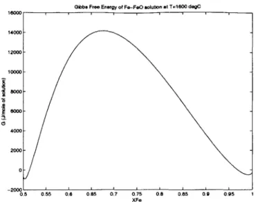
A free energy function for the Fe-FeO system was developed using the sublattice ionic liquid model from CALPHAD [11]. Gibb's free energy is plotted as a function of XFe in Figure 3.4.
Gibbs Free Energy of Fe-FeO solution at T=1600 degC 16000 --- 14000- 12000- 10000- 8000-4000 2000 0 --0.5 0.55 0.6 0.65 0.7 0.75 0.8 0.85 0.9 0.95 1 XFe
Figure 3.4: Free energy of Fe-FeO system using sublattice ionic liquid model
energies were set to zero. The figure shows a peak free energy of approximately G 2 14, 000 m
at XFe 2 0.68. The peak in free energy in terms of free energy density is
a and
/
become# = 16fpea = 2.72 * 1010 3 (3.42)
_18y 2
a = 6.6 * 10- 10N (3.43)
which gives an interface width of
C C 3.1 =4.8 *10-10m (3.44)
To track a one dimensional interface of this thickness on a solution domain on the order of 1cm would require on the order of 107 grid points. With such extreme length scales, modifications must be made to the diffuse interface model for practical use.
and 3 was found as a function of E. In terms of E, a and 0 become
3=
((18)
(3.1))(3.45)
(3.46)
This type of scaling is commonly called the phase field method.
3.2.2
Governing Equations
The equations given in this section are similar to the equations given for the sharp interface formulation. See Section 2.2 for a more detailed description of variables and terms. The Navier-Stokes equations were extended to the phase field model (see Jacqmin [10]) by adding an extra surface tension term. Conservation of x-direction momentum reads
a(pu)+
.(pfu)
= - 9e(Piu)+pgx+ V
)
-
ax
fV)
-
C9(3.47)
and conservation of y-direction momentum reads
a (PV) + V
(pv)
= -p + 9(77u)
+ pgy-2