Digital pulse processing

Digital Pulse Processing

by

Martin McCormick

B.Sc., University of Illinois at Urbana-Champaign (2010)

Submitted to the Department of Electrical Engineering and Computer Science

in partial fulfillment of the requirements for the degree of

Master of Science in Electrical Engineering and Computer Science

at the

MASSACHUSETTS INSTITUTE OF TECHNOLOGY

September 2012

@

Massachusetts Institute of Technology 2012. All rights reserved.

/Z

Author ...

...

...

Department of Electrical Engineering and Computer Science

July 19, 2012

Certified by...

... .. ...

6l V. Oppenheim

Ford Professor of Engineering

Thesis Supervisor

Accepted by ...

Professor teslil.

kolodziejski

Chair, Department Committee on Graduate Students

MASSACHUSETTS INSTfUE

OF 2ECW4 0L2OY

pT2~ 12,

Digital Pulse Processing

by

Martin McCormick

Submitted to the Department of Electrical Engineering and Computer Science

on July 19, 2012, in partial fulfillment of the

requirements for the degree of

Master of Science in Electrical Engineering and Computer Science

Abstract

This thesis develops an exact approach for processing pulse signals from an

integrate-and-fire system directly in the time-domain. Processing is deterministic and built from

simple asynchronous finite-state machines that can perform general piecewise-linear

operations. The pulses can then be converted back into an analog or fixed-point

dig-ital representation through a filter-based reconstruction. Integrate-and-fire is shown

to be equivalent to the first-order sigma-delta modulation used in oversampled

noise-shaping converters. The encoder circuits are well known and have simple construction

using both current and next-generation technologies. Processing in the pulse-domain

provides many benefits including: lower area and power consumption, error

toler-ance, signal serialization and simple conversion for mixed-signal applications. To

study these systems, discrete-event simulation software and an FPGA hardware

plat-form are developed. Many applications of pulse-processing are explored including

filtering and signal processing, solving differential equations, optimization, the

min-sum

/

Viterbi algorithm, and the decoding of low-density parity-check codes (LDPC).

These applications often match the performance of ideal continuous-time analog

sys-tems but only require simple digital hardware.

Keywords: time-encoding, spike processing, neuromorphic engineering, bit-stream,

delta-sigma, sigma-delta converters, binary-valued continuous-time, relaxation-oscillators.

Thesis Supervisor: Alan V. Oppenheim

Title: Ford Professor of Engineering

Contents

1 Introduction 7

2 Pulses as a Signal Representation 9

2.1 Basic Pulse Processing . . . . 12

2.2 A Signed Generalization of I&F . . . . 13

2.3 Methods for Reconstruction . . . . 15

2.4 Filter-based Reconstruction . . . . 17

2.5 Bounds after Pulse-domain Processing . . . . 20

3 Digital Signal Processing with Pulses 21 3.1 Discrete-time DSP (DT-DSP) . . . . 21

3.2 Continuous-time DSP (CT-DSP) . . . . 23

3.3 CT-DSP with Deltas . . . . 24

3.4 Linear Time-invariant Processing . . . . 25

3.4.1 Addition . . . . 26 3.4.2 Constant Multiplication . . . . 27 3.4.3 Delays . . . . 29 3.4.4 F ilters . . . . 29 3.4.5 Counting Networks . . . . 31 3.5 Piecewise-linear Functions . . . . 34 3.6 Absolute Value . . . . 34

3.7 Min and Max Operations . . . . 36

3.8 Choosing a Pulse Encoding . . . . 37

4 Error Sensitivity 39 4.1 Characterization of Pulse Timing Jitter . . . . 39

4.2 Characterization of Pulse Loss . . . . 40

4.3 Noisy Pulse Processing Machines . . . . 41

5 Applications 43 5.1 Sigma Delta Event Simulator . . . . 43

5.2 Filter Bank . . . . 44

5.3 The Min-sum Algorithm . . . . 46

5.3.1 A Pulse-domain Min-Sum Algorithm . . . . 49

5.3.2 Variable Nodes . . . . 49

5.3.3 Factor Nodes . . . . 50

5.4 Forward Error Correction . . . . 52

5.4.1 Pulse-domain LDPC Decoder Prototypes . . . . 55

5.4.2 Virtex II Implementation (internal tristates) . . . . 56

5.4.3 Virtex V Implementation (emulated tristates) . . . . 57

5.4.4 Simulations . . . . 57

5.4.5 Results . . . . 58

5.4.6 Hardware Resources . . . . 61

5.4.7 Alternative Form . . . . 62

5.6 _{Neural Networks . . . . 64}

6 Circuits for I&F Modulation and Processing 66 6.1 _{Frequency Modulation (FM) . . . . 66}

6.2 _{Neon-discharge Tubes . . . . 66}

6.3 Unijunction Transistor (UJT) Modulator . . . . 66

6.4 Neuromorphic Circuits . . . 68

6.5 _{EA Modulators . . . 68}

6.6 _{Quantum Modulators . . . . 70}

1

Introduction

Digital signal processing systems normally consist of a series of discrete-time operations applied to signal amplitudes represented by fixed or floating point binary codes. Signal representation is digital so that operations can be mapped to boolean functions and built out of switching circuits, while it is

discrete-time so that storage and processing is possible with a serial von-Neumann architecture. Little exception

is found even in fully-parallel ASIC signal processing systems. However, the processing of signals with digital hardware is not limited to this type of design. Instead, this thesis explores an alternative paradigm where analog signals are encoded as a series of digital pulses in continuous-time. These pulses are then processed accurately in the "pulse-domain" using special asynchronous finite-state machines before finally reconstituting an analog output signal.

The idea of pulse processing evokes the biologically-inspired neuromorphic computing systems pioneered by Carver Mead in the 1980's (e.g., [1]). However, what is explored here is different than these systems because most original neural systems forgo the use of exact timing structure in pulse signals. In fact, pulses are not even an explicit part of the processing in common analog VLSI implementations (where a surrogate analog signal indicates instantaneous rate). Later systems that actually employ pulses tend to use sophisticated biological spiking models but focus on increasing neurophysiological realism rather than understanding the significance for computation. For this reason, we break from being wed to biological models and return to a deterministic pulse encoding based on a straightforward generalization of the original integrate-and-fire model. Simple deterministic pulse encodings like this have seen renewed interest in light of the work of Aurel Lazar showing perfect reconstruction of an original analog signal from pulse times[2]. But while simple integrate-and-fire models receive renewed interested, methods for processing their pulses directly in a comprehensive way are not well understood.

A key contribution of this thesis is to reformulation integrate-and-fire into a digital signal processing framework so that a whole suite of pulse processing elements appear naturally. An important step is the recognition of a direct connection between integrate-and-fire and the bit-stream in sigma delta modulators. Sigma delta modulators are employed in sigma delta oversampled noise shaping converters and have con-tributed significantly to making transitions between the analog and digital domains inexpensive and accurate in modern DSP systems. Normally converters use digital filtering and decimation to convert the one-bit bit-stream of the internal modulator into a fixed-point (PCM) representation, however some work has shown that the bitstream itself is versatile for some classes of computation using simple circuits and without con-version to PCM[3, 4, 5, 6, 7]. Building on the work of these pioneers, this thesis takes the next step of removing the oversampling clock and processing asynchronously. This results in new processing elements that are both easier to analyze, and simpler to construct.

Only certain operations can be performed exactly with simple state machines in the pulse domain. However, there are distinct advantages when the necessary operations are available. Pulses are versatile in mixed-signal applications (demonstrated by the success of sigma delta in converters) and maintain some of the best features of both analog and digital. Pulses still possesses the immunity to noise-floor and transistor variation, modularity, and reuse of a digital format but exhibits the circuit simplicity, single-wire data path and power efficiency attributes of analog circuits. Removing the clock allows true continuous-time computation giving computational benefits when solving differential equations and certain optimization and inference problems. Asynchronous operation also reduces overall power requirements and electromagnetic interference from periodic clock waveforms. Pulses are also more robust to digital errors than a traditional PCM format. Pulse loss, insertion and jitter are the only types of error in a pulse signal and all of these errors impart small distortion on the encoded signal. Applications such as multimedia signal processing, user interfaces and prosthetics, sensor networks, and algorithms for optimization and inference that tolerate small error can have a very significant reduction in the design size.

The organization of the thesis is as follows. In chapter 2, we examine deterministic pulse signals and their connection to random point processes. While there are numerous ways to encode a continuous-time

waveform into a sequence of pulses, a specific generalization of integrate-and-fire is chosen because (1) it is a simple fundamental model (2) an encoder is readily built with basic electrical circuits (3) it admits accurate and robust operations directly in the pulse domain and (4) the original waveform can be reconstructed within fixed bounds only by filtering the pulses. These factors make the encoding desirable for practical pulse-domain processing tasks. The encoding is then generalized by using an equivalent model consisting of a cascade of an integrator, uniform quantizer, and differentiator. This provides both an intuitive model for integrate-and-fire and a new generalization that includes negative pulses. From the pulses of this system, a quantized version of the integral can be reconstructed with an up/down counter. While the quantization incurs a loss of information, it indicates bounded intervals that the encoded signal's integral must lie within. These bounds become a critical tool for analyzing approximate reconstruction and designing pulse-domain processing systems.

In chapter 3, continuous-time digital signal processing (CT-DSP) is introduced as an application for pulse processing. CT-DSP is similar to traditional discrete-time DSP but removes the sampling step and processes digital signals asynchronously. Yannis Tsividis has recently led the investigation into analysis and construction of CT-DSP circuits (see [8]). A number of benefits including the elimination of aliasing and reduction of power consumption are obtained this way. However, the completion logic and handshaking associated with asynchronous logic add complexity to the design especially when fixed-point (PCM) digital representations are used. Instead, by representing signals with digital pulses on single wires, many of the complications are eliminated. We suggest an aggressive simplification by using new pulse-domain circuits that leave out handshaking completely at the expense of occasional random errors. The integrate-and-fire encoding is found to be naturally robust to these errors for many types of processing. The operations for addition, constant multiplication and delay are derived and connections are made to early A-domain circuits for the same operations. For each operation, the change to the reconstruction bounds are shown. After the developed pulse-domain operations, a unique method for constructing pulse-domain filters is introduced. A key structure used to implement the filters is a counting network-a network of interconnected balancer components studied in theoretical computer science. Counting networks perform the counting operations in pulse-domain circuits in a distributed fashion, making them particularly robust and efficient. Finally, the general class of memoryless CT-EA operations are found. This is the set of all operations that can be performed using only an asynchronous finite state machine that passes or blocks pulses. It is shown that these are the positive homogeneous functions of order 1. In particular, this includes piecewise linear operations such as absolute value, min, and max. These functions greatly expand the type of applications possible in the pulse domain.

In chapter 4, the distortion of pulse signals is considered. Distortion is classified as either pulse loss and insertion or pulse timing jitter. The frequency-domain effects of these two types of errors on reconstructed signals are examined for pulse encodings. In addition, the effect of pulse timing jitter on the input to pulse processing circuits is considered. Extremely jittered inputs are modeled as Poisson processes and the asynchronous finite-state machines are interpreted as Markov chains. The state evolution of each is then a continuous-time Markov process from which a solution to the output rate is derived. It is found that many of the pulse-processing circuits still give good approximations of their operation despite the timing jitter.

In chapter 5, applications of pulse-process are built and analyzed. Simulations are performed using custom discrete-event simulator software and FPGA hardware. Applications include a pulse-domain filter bank, a quadratic program solver, the min-sum algorithm, and an LDPC decoder. The decoder, in particular, outperforms the state of the art in fully-parallel digital decoders under a number of metrics.

Finally, chapter 6 briefly examines circuits for implementing pulse modulation and processing. A precise connection between integrate-and-fire and the sigma delta modulator is made. In addition, a variety of potential pulse processing technologies are examined from CMOS to single-electron devices.

2

Pulses as a Signal Representation

While continuous functions and differential equations dominate the classical laws of nature-many fundamen-tal phenomena are better modeled as a series of pulses. Raindrops, for example, produce a series of pulses that can be recorded by marking points in time. A simplified model measures each drop with an equal weight over an infinitesimal instant. The resulting pulse signal is then a temporal point process.

A point process is most often studied as a type of random process. In particular, rain is treated as a Poisson process. With a Poisson process of a given rate, knowing one drop's exact time is inconsequential in guessing the time of any other. The model for a Poisson process consists of a coin-flipping experiment where a heads indicates a pulse. An independent coin flip occurs every dt seconds and the coin is weighted to have a probability of heads A -dt. When dt is made infinitesimal, flips are rapid and heads occur at random instants in continuous time. The pulses form a Poisson process with an average rate of A heads/second while the exact time between any two consecutive pulses follows a probability distribution, P(r) = Ae-.

In general, Poisson processes are non-homogeneous where the average rain rate-or probability of heads-changes in time. Here, rate is represented by a continuous function, A(t). Non-homogeneous Poisson processes include the incidence of photons on the retina (A(t) corresponds to a changing light intensity), clicks of a Geiger counter measuring radionuclide decay events (A(t) falls as the radionuclides diminish) or electrons passing across some cross-section in a wire (A(t) is the electric current).

In all of these examples, the point process is formed from the combination of many independent pulse-generating sources. Indeed, formally a Poisson process always arises from the superposition of many inde-pendent equilibrium renewal processes. If each source has a small rate and is measured without distinction, the merged pulses behave asymptotically like a Poisson process. This is an important theorem attributed to C. Palm and A. Khintchine[9] that explains it's widespread appearance in natural and man-made systems.

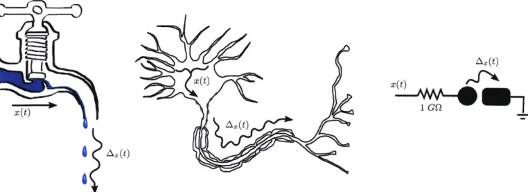
However not all pulse phenomena are Poisson processes or random; in many systems, pulses follow a deterministic process. For example, if rain collects together and spills off a ledge forming drips that fall to the ground, the pattern is regular-it is easy to predict the next drop from the last. If the rain falls faster, the drip rate follows but the regularity is maintained. Regular dripping is an example of a relaxation oscillator. The simplest relaxation oscillator example is the dripping that comes from a leaky faucet. Water molecules slowly flow through a faucet valve and collect at the edge of the tap in a bead of water. The molecules accumulate until their collective weight exceeds the grip of surface tension (N ~ 2 x 1021 molecules), then the complete drop falls and the process begins anew. Here, the formation of pulses is different from the

Poisson process. In fact, pulses are formed in the limit of decimation rather than merging. The relaxation oscillator can be modeled as decimation of random input pulses (water molecules flowing in) by a factor N where input pulses are counted and every Nth produces an output droplet. A state machine for this process is shown below.

r~j

In the limit where both the input rate A and the decimation factor N are large but the ratio is held

A1

constant, the output rate is y = pulses/second with exactly 1/p seconds between consecutive pulses1. This type of relaxation oscillator has a variety of names from different fields of study. Perhaps the most well-known is "integrate-and-fire" after the model of neuron action potentials attributed to neurophysiology pioneer Louis Lapicque[10]. In the equivalent non-leaky integrate-and-fire model (I&F), a constant input rate signal x(t) = A is integrated until a threshold A = N -dt is reached, at which point an output pulse is generated and the integrator is reset to zero. This process is illustrated in Figure 2.

x(t) AX(t)

X(t)

AX(t)

ft

f t

Figure 2: The non-leaky integrate-and-fire model (I&F).

In general, I&F can modulate any non-negative time-varying input x(t). Similar to the Poisson Process, this is clearly a type of pulse-frequency modulation. However, while a Poisson process is inherently random, I&F pulses are formed deterministically from x(t). In particular, the pulses are spaced such that the definite integral of x(t) between consecutive pulse times is always exactly A. This integral is concentrated into a Dirac delta of measure A to represent an output pulse in A,(t). The integral of x(t) and A,(t) are always close-I&F simply delays some of the integral mass by concentrating it at these specific points in time.

'Regular pulsing from decimation follows from the law of large numbers. If the original input pulse signal is Poisson at rate A, the time between pulses r is an exponentially distributed random variable with P(r) = Ae-Ar. After decimating by a factor N, the time between pulses is T ~ Erlang[N, A]. As N and A are made large but A is held constant, r ~ [ ]. In the limit, the variance

P(r) drops to zero and the pulse spacing is concentrated at r = N/A.

X t) x ") xx~t)

Figure 3: A dripping faucet, biological action potentials and the Coulomb blockade all exhibit integrate-and-fire. I&F is an excellent model for a variety of natural and man-made systems spanning physiology to physics. The faucet is an I&F system where turning the handle slightly modulates the leak x(t) and changes the drip rate. In this case, the drip sizes remain constant but the the time between drips changes depending on x(t). Lapicque's model of neuron behavior is also an important example[11]. In a neuron, there is a large difference in concentration of sodium ions (Na+) and potassium ions (K+) between the inside and outside of the cell wall maintained by sodium-potassium pumps powered by ATP. Different neurotransmitter stimulus at the dendrites of the neuron allow Na+ to leak in at rate x(t) and accumulate at a cell region called the axon hillock. These ions raise the voltage potential across the cell's membrane as charge integrates. In the axon hillock, there are many voltage-controlled ion channels that selectively allow Na+ into the cell or K+ out of the cell. Once a threshold of about A = 15mV is met (around 1010 ions), a runaway positive feedback loop of Na+ channels opening permits further sodium influx and raise the voltage to 1OOmV. However within about 1ms, the K+ channels open and the Na+ channels close and the out-flux of K+ lowers the voltage back down just as rapidly. The complete cycle is an action potential and forms a sharp voltage spike that is repeated down the axon to signal other neurons.

The vibration of the vocal chords (folds) in animals can also be modeled as integrate-and-fire[12]. As intraglottal pressure builds it eventually opens the vocal folds at a certain threshold causing a short burst of air before closing again. This repeats to form regular glottal pulses. The rate of pulses determine pitch.

Integrate-and-fire also occurs at the quantum level with single-electron tunneling. At low temperatures, the Coulomb blockade effect[13] occurs when current flows through a large resistance to an island and encounters a barrier to a lower potential. The barrier behaves as a capacitor that charges over time. After the island voltage exceeds the barrier, a single electron tunnels across. Further tunneling is then blocked until the island is refilled from fractional electron diffusion across the resistor. (Fractional diffusion is interpreted as the electron wavefunction evolving across the resistor). Very regular single-electron tunneling occurs at a rate proportional to the applied x(t) voltage[14]. I&F is also found elsewhere in quantum systems, including photon anti-bunching observed from single-molecule sources[15].

This I&F process is also used in many classical electrical systems. Zero-crossings of frequency modulated (FM) signals and clocked Sigma-Delta (EA) oversampled noise-shaping converters have a direct correspon-dence to I&F (see Chapter 6). These different viewpoints of the same phenomena are useful for understanding and building pulse modulation and processing elements.

2.1

Basic Pulse Processing

One of the key objectives of this thesis is to develop ways to process pulse signals directly. In order to develop an intuition for how pulse-processing elements might be constructed, we give a brief example for comparing the pulse rates of two signals. We see that the structure of I&F makes it more amenable to computation. For example, in Figure 4 two Poisson and two I&F signals are generate with constant rate inputs B and A. For I&F, determining the greater input from the pulses is simple: two consecutive pulses without interruption by another indicates that that pulse signal encodes a larger value. Conversely, with Poisson processes long-term averages are required to make even a probabilistic statement about relative rate. The "uninterrupted pulse" method of rate comparison for I&F pulses is particularly convenient because it

A

_{Ihm It}

it 1

At 7- Poisson B Poisson A --- I&F

lttt

it it it

it it it it it

B - ti t2

Figure 4: The regular structure of I&F assists in computation. Two consecutive (uninterrupted) pulses at ti and t2 indicate that input B > A.

obviates the need for another time source. (while the time between pulses could be measured to determine that B has a shorter period, measuring time requires another more rapid pulse reference-a clock). Instead,

detecting uninterrupted pulses only requires a single bit of state indicating which signal pulsed last. Even when I&F inputs are time-varying, certain information about the encoded signal can be ascertained from the pulse times. Two consecutive pulses indicate that the definite integral of x(t) is exactly A over the time interval that they enclose. If consecutive pulses are not interrupted by a pulse from another signal, the definite integral of the other encoded signal is less than A over the same time interval (otherwise it would have interrupted with a pulse). This implies that the signal average for one is higher than the other over the interval. This fact hints at a possible pulse-domain max operation for time-varying I&F inputs. Still, it is not immediately clear how this or general operations can be performed exactly in the pulse-domain or whether any guarantees can be made about their performance.

Before tackling the general processing problem, we first generalize I&F to support signed inputs (x(t) < 0) by adding an additional negative threshold to the modulator. The output Ax (t) then includes both positive and negative pulses. A formulation of signed I&F is easily interpreted from a digital signal processing perspective. This perspective ultimately leads to a method for constructing a broad class of pulse-processing elements.

2.2

A Signed Generalization of I&F

An equivalent form of I&F is found by noting that the process is quantizing the integral of x(t), with a pulse emitted whenever the integral reaches a new multiple of A. Indeed, this is precisely a cascade of integration, uniform quantization and differentiation with respect to time. This process is shown in Figure 5.

f

XWt

Xrr t)

d

IA

t

Quantizer

Figure 5: An equivalent representation of I&F, also called here continuous-time EA (CT-EA).

The outpfit of the integrator X(t) is a continuous function that may cross up or down through at most one quantizer level at any moment. The quantizer output is time-varying quantized function and the derivative of this function contains a Dirac delta whenever a change in level occurs. To be explicit, we define a function for each stage of the process. The output of the integrator is written as convolution by the Heaviside step function u(t),

X(t) u(t) * x(t) = x(t') dt'

/-o

The uniform quantizer has levels spaced by A. Quantization applies the floor function to an input signal,

X(t)

= Q(X(t))

- LX(t)j

=

AL

_A

JM

The output of the quantizer X (t) transitions to a new value immediately when X (t) enters a new quantization interval. The transition causes the differentiator to produce an output transient. Specifically, a Dirac delta of measure

+A

is produced when transitioning up a level and a Dirac delta of measure -A is produced when transitioning down a level.

A(td) =-(t)

dt

While I&F normally only supports x(t) > 0, this formulation clearly extends to x(t) < 0. Negative pulses are simply emitted when the integral of x(t) decreases through a multiple of A.

From A2 (t) one can reconstruct the quantized integral X(t) by integrating the pulses X(t) =

u(t)

* Ax (t) (e.g., with an up/down counter). As before, the definite integral of x(t) over the time period between two consecutive positive pulses is exactly

+A

(because the integral has increased by one quantization level). However, now there are additional combinations of pulse signs. The definite integral of x(t) between two negative pulses is exactly -A (because the integral of x(t) has decreased by one quantization level) and between pulses of opposite signs the definite integral is exactly 0 (because the integral of x(t) has crossed the same level back again). In general, the quantized integral equals the original integral exactly (i.e., X(to) = X(to)) at two times: immediately following positive pulses and immediately preceding negative pulses. Therefore, the definite integral of x(t) over an interval between any two pulses can be computed from the integral of the pulse measures within (and bordering) the interval.

This generalization of I&F can be returned to a feedback form as before by only storing the relative position of the integrator state within a single quantization interval. To show this, the process of quantization is first written as subtraction of a gap signal g(t),

9(t)

+ Z(t

Quantizer

4F

LI

Figure 6: A continuous-time uniform quantizer represented by subtraction of a gap signal, g(t) E [0, A).

AX(t)j g(t)= X(t) - A L J

= X(t) mod

A

The gapi g(t) is the amount that X(t) exceeds its quantized value-a quantity bounded by the interval [0, A). At any time, to, the future output of the I&F modulator depends only on the integrator state at that time, X(to), and the future input {x(t) I t > to}. However, any offset of nA, n E Z is an equivalent integrator state value relative to the periodic levels of the quantizer. Therefore, subtracting an integrated count of the output pulses,

Z(t)

= u(t) * A2,(t) has no effect on the modulator operation. The resulting difference is the gap g(t) and is all that must be stored to determine pulse times. Only two comparisons of g(t) are needed-whether g(t) > A and whether g(t) < 0. When g(t) = A, a positive output pulse is subtracted setting g(t) to 0. When g(t) = -c, a negative output pulse is subtracted resulting in g(t) = -E + A.

II x(t)

X (t)Zt)2()

J

7t

Quantizer

4A 3 A I I lX to) A Equivalent states 2A

*)

0 1F

AX

t)o

AX(t) x(t)

---

I A - g(to) :to

AX(t)

Figure 7: A feedback structure is formed by subtracting integrated within [0, A).

1

The negative gap, -g(t), is commonly called the quantization error.

output pulses. The difference g(t) remains

9A 7A 6A 4A 3A 2A 1A r

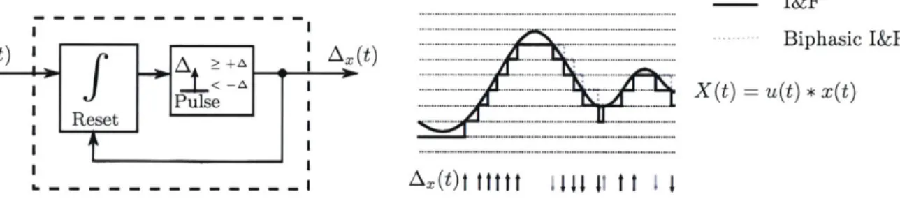
---The feedback structure is simplified by moving the two integrators across the subtraction to form a single integrator. This integrator is reset to 0 when a positive feedback pulse is subtracted or set to A - E when a negative pulse is subtracted. The feedback loop is identical to the original I&F for inputs x(t) > 0.

x(t) -

f

g(t) AX (t)

Pulse

Figure 8: The signed I&F modulation using only a single integrator.

This generalized I&F modulation is the primary pulse encoding used throughout the thesis. The reader who is familiar with EA converters may recognize a similarity between I&F in Figure 8 and the first-order EA modulator inside converters. Indeed, there is a direct correspondence between the two. A EA modulator circuit can be used verbatim to perform the I&F modulation and only produces slight pulse timing jitter (aligning pulses to the clock period). An exact relationship between I&F and EA is examined in Chapter 6. Also, some readers may recognize Figure 8 as similar to biphasic integrate-and-fire (e.g., [16]). The only difference is that biphasic I&F uses a lower threshold of -A instead of 0. This mitigates the problem of being sensitive to perturbation when X(t) is close to a quantizer threshold (the modulator may generate a rapid series of pulses with alternating signs as it moves back and forth across the threshold). Biphasic I&F resolves this problem because the feedback pulses reset the integrator to 0 for both the

+A

threshold and the new -A threshold. Biphasic I&F skips a single output pulse (compared with the I&F described here) whenever the integral changes direction through a threshold (i.e., x(t) changes sign). This is illustrated in Figure 9. Skipped pulses always alternate in sign and are self compensating. In practice, the distortion is negligible and a biphasic I&F circuit can be used for most processing despite the difference.

- I&F

x.t)...A... Biphasic I&F

< - .X(t) =u(t)* x(t)

Reset Pulse

R eset ---- ...-...

Figure 9: Biphasic I&F is a stable modulator that differs by skipping a pulse during the first of each sign change.

2.3

Methods for Reconstruction

The I&F modulation converts a signal, x(t), into pulses indicating times when the signal's integral, X(t) passes through integer multiples of a unit A. Based on these times and directions, can the original signal be reconstructed exactly? To answer this question, we first formally define the pulse signs and times,

tm C {r X(r) = {. .. ,-2A, -A,0, A, 2A,...}}

The pulse signal is defined by a sum of weighted Dirac delta functions, AX(t) = sn -) c(t - tM)

A signal x(t) is consistent with an I&F encoding A.,(t) if the following bound holds for all times t,

0

< u(t) * x(t) - u(t) * Ax(t) < A, Vt

10A

8A

7A

6A

-M

Equation (1)

Xi(t) = u(t) * Xi(t) Xi(t)

AX (t)

5A I

4A

-It is apparent that I&F modulation is a many-to-one mapping due to the information loss from quantization; many x(t) signals are consistent with a given sequence of tm and vm. For example, Fig-ure 10 shows three signals with integrals that lie within the bounds defined by a single Ax(t); all three have the same I&F encoding. Consequently, unique recovery of x(t) from A- (t) is not possible in general. However, if x(t) has limited degrees of freedom, solving a system of equations may lead to an exact reconstruction. For ex-ample, for certain bandlimited x(t), there is a system of equations that is well conditioned if the average number of pulses exceeds the Nyquist rate of x(t). In our case, I&F is one of the general time-encoding machines studied by Aurel Lazar[2].

Following Lazar's work, recovery involves constructing a linear system of equations that capture the constraints on possible x(t) imposed by the pulse times and signs of a given Ax(t). In the case of I&F, a subset of the constraints implied by Equation 1 are used. Specifically, we assert that the definite integral of x(t) between two consecutive pulse times tm and tm+1 is a specific value (either -A, 0 or +A depending on the two pulse signs),

2A

-

1A-Figure 10: The three signals xi(t), x2(t) and X3(t) have identical A,(t) but only one is bandlimited.

tm+1 qm= x(t)dt = X(tm+1) _{- X(tm)} +A, if m± = +A _ -A, if Vm = -A 0, if m± = +A 0, if Vm = -A and vm+1 = +A and vm+1 = -A and vm+1 =-A and vm+1 = = (vm + vm+1)/2

Now if x(t) is bandlimited and has only finitely many non-zero samples, it can be written as, x(t) = Ec" - #(t - s')

n

where s, = nT are uniform sample times, c, are a series of sample values and

#(t)

= sin(27rt/T)/(7rt). Constraints are written as q = 4cwhere qm c {-A, 0,

+A}

and Chmn =

im+1 #(t

- s,)dt. The elements of 5*

can be solved by computing the pseudo-inverse of (P and evaluating 6= 44. The solution is unique as long as m > n and 4 is full rank. The conditioning can be further improved if the s, are chosen non-uniformly. Unfortunately, there are some practical disadvantages with this reconstruction method. The pseudo-inverse is computationally expensive and calculating the matrix 4 involves non-trivial definite integrals.

If the encoding is biphasic I&F, q, = vm+1.

16

Furthermore, reconstruction solutions are sensitive to pulse loss, spurious pulse gain or strong timing jitter. Even more importantly, this reconstruction method cannot accept a more general class of I&F pulse signals

produced during pulse-domain processing. For these reasons, a simpler form of reconstruction is studied.

2.4

Filter-based Reconstruction

For the purposes of this thesis we propose a simpler (but approximate) I&F reconstruction that uses linear filtering. The pulses in A.,(t) are passed through a lowpass filter so that each pulse is replaced with the filter's impulse response to form a continuous output signal. While the reconstruction is inexact, for certain filters the results are very close and the output error can be bounded to a small interval in the time-domain. To see this, note that the pulse signal A,,(t) is a superposition of x(t) with the gap signal's time-derivative

g'(t),

AX(t) = - (X(t) - g(t))_dt

= x(t) - g'(t)

The quantization gap g(t) exhibits a broadband power spectral density for most inputs. After differentiation,

g'(t) = -g(t) has a high frequency power spectral density. An example is pictured in Figure 11.

9'(t) Fg()|

t _f

Figure 11: An example of g'(t) = g(t) and its power spectral density.

Intuitively, applying a lowpass filter to Ax(t) removes much of -jg(t) and restores a lowpass filtered version of x(t). Indeed, for certain filter impulse responses, filter-based reconstruction maintains a time-domain error below a fixed bound. To see this, note that the bounds on g(t) imply,

UMt * (XMt - AX(t)) = X(t) - 0(() = g(t) C [0, A), V t

This directly implies a bound between the moving averages of x(t) and Ax (t). The moving average is defined as convolution with a rectangular window of width W,

w(t) u(t) - u(t -W)

The moving average of x(t) and Ax(t) are labeled x,(t) and A,(t) respectively,

x.(t) = w(t) * x(t)

AW(t) = w(t) * AX(t)

The error between xw(t) and Aw(t) is,

ewM) = xw(t) - AW(t)

= W(t) * g'(t)

g(t) - g(t - W) A A

= W W' WT,

This error is is also bounded. Therefore, the moving average of Ax(t) x(t). The error between them has bounded infinity-norm,

Vt, W

is always near the moving average of

||e(t)O < A_W

The bound can be tightened by increasing the width of the filter W or decreasing the threshold A. In particular, as W -> oo, the error goes to zero, implying the averages of x(t) and A. (t) are equal. The tradeoff

with moving-average reconstruction is that for larger W the bound applies to an increasingly narrow-band version of x(t) so that only the low frequency components of x(t) are accurately recovered.

ew(t) = xw(t) - Aw(t),

Ie

(t)| o < A

Figure 12: An example of I&F modulation and reconstruction using a moving-average filter.

Moving-average reconstruction is non-ideal due to the undesirable sinc-shaped frequency response of the filter. While the time-domain bounds are good, the output Aw (t) is blocky and still contains significant high-frequency error. Fortunately, additional filtering can improve the overall reconstruction high-frequency response

while maintaining error bounds in the time-domain. If an additional filter with impulse response h(t) is applied, Xh(t) = h(t) * x,(t) Ah(t) h(t) * A,(t) The error, eh(t) Xh(t) - Ah(t) = h(t) * e,(t)

This new error is bounded as well. Convolution of any two absolutely integrable functions obeys Young's inequality,

|h(t) * e,(t)||o < ||h(t)||1 |lew(t)||o

Therefore,

leh(t)||oo < -||~h(t)J|1 W

So that eh(t) has the same bounds as es(t) but scaled by the absolute-integral of h(t).

One of the most straightforward reconstruction filters consists of repeatedly computing moving averages. We define 0(n) (t), called a B-spline of degree n,

# (t) = w(t)

-(t)=w(t) * w(t)

(t) = w(t) * #C4-l)(t)

Because (n) (t) = 1 for all the splines, reconstruction error from any of them has the same bound, ||")(t) * (x(t) - AX(t))||, < A V n, t, W

-W

While the strict time-domain bounds remain the same for all orders n, the average error power tends to diminish as the order is increased. In general, higher-order B-splines have better frequency-domain characteristics that approach a Gaussian in time and frequency. An advantage of B-splines is that they are easy to implement in discrete-time. A decimation filter commonly employed by EA converters is the sinc3 filter. This filter, named for its frequency response, is the B-spline of degree 2 and is implemented as a cascade of 3 counters (integrators) followed by 3 first-differences at sampling rates with progressively greater decimation. Besides B-splines, nearly any low-pass filter does a good job at reconstructing the input from pulses-even if a time-domain bound cannot be given directly.

Compared with the exact reconstruction methods, there are a number of advantages with the filter-based approach. When a filter is used for reconstruction, the I&F pulse encoding is robust to pulse loss or spurious pulse insertion because each pulse contributes the same small weight in the reconstruction. If a pulse is lost at a given time to, the error only affects the reconstructed signal when the filter window encloses to. As it passes by, the error no longer contributes and the original bounds still hold. In addition, the reconstruction is a linear time-invariant operation and hints that pulse-domain computation can be performed before reconstruction. For example, adding two pulse signals and then reconstructing the result with a filter is equivalent to adding the individual reconstructions due to the linearity of filtering.

2.5

Bounds after Pulse-domain Processing

When processing in the pulse domain, the effective gap g(t) on a resulting pulse signal may exceed the original range [0, A). For example, adding two pulse signals causes the reconstruction's error bounds to add as well. To keep track of the range of values possible for the gap between a signal integral and its pulse encoding integral, a more general upper-bound variable AU and lower-bound variable AL are introduced. A pulse signal Ay(t) is said to satisfy the bounds {AL, AU} as an I&F encoding of y(t) if,

u(t) * (y(t) - AY(t)) E [-AL, AU), Vt (2)

gy(t

Likewise a signal y(t) is said to be consistent with Ay(t) under bounds {AL, AU} if (2) holds. When a pulse signal has these generalized gap bounds, the filter-based reconstruction A, (t) = w(t) * Ay (t) has accuracy,

AL+AU AL AU

yw(t) - Aw(t)G (E -A A ) Vt (3) The output of an I&F modulator with threshold A is a special case where the gap bound values are AL = 0 and AU = A. These bounds {AL, A U} will change as the pulse signal undergoes various operations. The bounds of a given operation's output are determined by the type of processing operations performed and the bounds of the input pulse signals. Certain operations will expand the gap while others will contract it. In this thesis, every time a new pulse-domain operation is defined the exact operation being performed along with the output bounds as a function of the input bounds are given in a boxed form. For example, the process of merging multiple pulse signals is stated as,

Y i (t i Y i

It is particularly important to keep track of these bounds because input bounds to a pulse processing operation often determine the number of states in the state machine. In particular, general piecewise linear operations vary their design depending on the input bounds.

Occasionally, additional random noise or processing error may remove or insert a single pulse in AY(t) that results in temporarily violating the bounds. These 'exception points' will not be included in {AL, AU} directly because they are temporary, are often rare, and complicate the analysis. In any case, the potential for exception point errors from processing will always be identified. In the end, the actual reconstruction error is proportional to both the bounds and the number of spurious exception points in a given window.

3

Digital Signal Processing with Pulses

By interpreting the integrate-and-fire modulator as the cascade of an integrator, uniform quantizer, and a differentiator, many pulse-domain operations are easily derived by applying traditional DSP operations on the encoded integral. A key difference from DSP is that the operations occur immediately in continuous-time rather than at a regular sampling intervals. While this may at first appear to be dramatically different than discrete-time processing, the analysis of continuous-time DSP operations is straightforward. Before developing the pulse operations, a short discussion illustrating the differences between discrete-time and continuous-time DSP is given. The following explanation is based heavily on the work of Yannis Tsividis [8] who has pioneered the modern study of continuous-time digital signal processing (CT-DSP) systems. After this review, pulse-domain operations for addition, constant multiplication and delay operations are developed, followed by a general set of piecewise linear operations.

3.1

Discrete-time DSP (DT-DSP)

Traditional implementations of digital signal processing in fully-parallel ASICs are synchronous. This is because of the way boolean functions are implemented with switches. The gates and wires in a circuit have finite delay so that when an input to the boolean function changes, different bits in the resulting output code may take varied amounts of time to transition to their new value. The meaningless intermediate codes are glitches that are passed on to the next circuit. If there is ever a feedback loop, these glitches will accumulate so that digital signals become meaningless. The consequence of synchronous design methodologies for signal processing systems is the need for discretization of the signal in time through sampling.

Normally, a fixed-point discrete-time DSP system contains three stages: A/D conversion, synchronous digital processing and D/A conversion. We will consider the mathematical formation of the three stages and then investigate how the removal of sampling modifies the process. A/D conversion consists of quantization and sampling. As before, if we assume a uniform quantizer with levels spaced by A, quantization consists of applying the following function to an input signal,

(t) Q (z(t))

A

ALX(t)I

A

Again, the difference between the quantized and unquantized signal is called the gap, 9x(t) =z(t) - A[(t)_A

The quantization function is a memoryless nonlinearity so that the frequency spectrum of gx (t) has broadband frequency components. For example, if x(t) is a single sinusoid, g.(t) contains harmonics at integer multiples of the frequency.

While the output of the quantizer may transition at any instant, the sampling step only measures new values at sample times. Sampling is equivalent to multiplication of the signal by a regular impulse train s(t) with sampling period T seconds,

00

Multiplication by s(t) only captures the quantized signal at multiples of the sampling period T. The values at these times can be represented by ,[n] =r(nT). Multiplication by s(t) results in,

z, (t) = __ (t) -s (t)

00

S:

,[n] J(t - nT)

The weighted periodic pulse train x, (t) is entirely described by the quantized pulse weights

2[n]

that can be represented as a sequence of binary codes and processed synchronously by a DSP.

A frequency-domain representation of sampling indicates that periodicity is introduced in the signal's frequency components. The Fourier transform of a periodic pulse train s(t) is also a periodic pulse train,

1 m0

S(f) =

L:

f6 - )

T Tc

M=-oo

The period of this pulse train is the sampling frequency, 1. Multiplying by s(t) produces a signal with Fourier-transform consisting of a superposition of shifted copies of the original signal's Fourier transform, i.e. aliasing,

Xs(f)4= T (f -m4)

m--oo

If J(t) is band-limited to half of the sampling frequency, these copies will not overlap and Xs(f) X (f) over an interval

f

C [--, -]. For this reason, most systems include an analog anti-aliasing filter at the beginning of the conversion process to remove noise and other interference at higher frequencies. However, despite an anti-aliasing filter, the subsequent quantizer non-linearity always adds an infinite-bandwidth signal g(t). After sampling, all of the broadband components of gx(t) alias into the interval

f

E [- -, -]. The compounded power spectrum is fairly flat over the interval and is often approximated as white[17]. The quantization error power can be reduced by decreasing the quantization interval A or oversampling the input signal. Oversampling spreads the aliased quantization spectrum thinner over a larger bandwidth and allows more to be removed by filtering. For example, if gx[n] is assumed white, doubling the sampling rate allows a low-pass filter to reduce in-band SQNR by about 6dB.

Once a sequence of codes I[n] is available from A/D conversion, a synchronous digital signal processor can manipulate them arbitrarily. An important class of DSP computation is linear time-invariant (LTI) filtering-convolving the input sequence of numbers -[n] by some desired impulse response sequence h[n] to form y[n] = ±[n] * h[n]. The resulting sequence y[x] is then converted back to a periodic output pulse train. This process is exactly equivalent to continuous-time convolution of the input pulse train

I-

(t) by a fixed periodic pulse train with programmable weights,

hs(t) = h[n] .6(t - nT) n

The periodic pulse signal h,(t) is the response of the DT-DSP to a single input pulse 6(t). By linearity and time-invariance of the processing, the response to an input x,(t) is,

yS(t) = y[n] .6(t - nT) n

= x8(t) * hs(t)

The digital LTI filter effectively applies a filter with impulse response h, (t). The effective frequency response of the DT-DSP is then,

Hs(f) = 5h[n] .e-2,fnT n

This frequency response is periodic in the clock frequency 1. With the selection of weights h[n], the DT-DSP chain can give any desired frequency response over the interval

f

e [- , ]. The signal ys (t) is then passed through an analog anti-imaging filter with bandwidth -. The complete process is illustrated in Figure 13.

Discrete-time A/D Converter (DT-ADC) Discrete-time D/A Converter (DT-DAC)

Pulses to Digital code|

Analog X digital code + + sequence Analog

filter sequenceto pulses filter

Quantizer x 1 x a x

(t) -- , -

-Figure 13: A depiction of discrete-time digital filtering with h[] ={,

j,

}}.

3.2 Continuous-time DSP (CT-DSP)

While not usually considered, the sampling process in DSP can be eliminated and a quantized input signal can be processed in continuous-time. Continuous-time digital signal processing (CT-DSP) is a name introduced by Yannis Tsividis for this process. Ostensibly this involves a quantized signal represented by codes that change value at arbitrary times. When the A/D quantizer changes levels, the new code is immediately processed asynchronously by the signal processing system. This processing is indeed feasible in a fully-parallel ASIC if the issue of erroneous glitches can be resolved.

In an idealized CT-DSP model, everything operates like a typical discrete-time processing circuit except that addition and constant multiplication circuits update their digital output codes immediately in response to a changing digital input code. Changes in codes do not suffer from glitches or timing variation between bits. A controlled digital delay of an entire code is also used to build LTI filters. If these controlled delays are all a fixed time T, the CT-DSP impulse response can be exactly the same as a DT-DSP. However a CT-DSP can also be generalized to include arbitrary delays. Now, the response may be a general aperiodic pulse signal,

hcT(t) = h .6(t - t7)

Both the weights hn and the delays t, can be chosen arbitrarily. The resulting frequency response HOT(f) is no longer periodic in the clock frequency,

HcT(f) hn -e-j3 .

The extra freedom with the tn's allows more flexibility in the filter design. Filters can be constructed with fewer taps and can give a desired response over any band with the proper selection of delays.

In principle, a CT-DSP can be constructed using asynchronous circuits. Asynchronous digital design has remained less popular than clocked approaches but has found success in certain applications where benefits outweigh the increased design complexity. Quasi-delay insensitive (QDI) circuits are relatively common and make only slight timing assumptions. In such circuits, typically two or four phase handshakes and completion logic are used where modules assert their readiness to accept or send data, and acknowledge full reception of the data. This introduces extra delay for messages to be sent back and forth and also excess circuitry-often doubling the number of transistors in a design[18]. However, this can still be worthwhile for the benefits of asynchronous operation. The removal of a clock can reduce power consumption by about 70%. A CT-DSP system only performs switching when the quantized input changes, making the dynamic power consumption low and a function of the input signal. Without discretization of time, a CT-DSP also generates less in-band quantizer distortion and eliminates the disadvantages of sampling.

Yannis Tsividis et. al. have recently led the investigation into CT-DSP systems. Authors have proposed an A/D converter that maps an analog input into a continuous-time digital representation and processes the information without a clock. Computation is done with clever asynchronous circuit techniques and handshaking between modules. For example, a continuous-time FIR and wave-digital filters using tunable continuous-time digital delay elements was demonstrated in papers by Schell, Bruckman and Li [8, 19, 20, 21]. Observed benefits of CT-DSP include,

" Reduced in-band quantization noise and alias-free nonlinear signal processing. " Circuit power consumption that depends on the activity of the signal.

" Extra degrees of freedom in delay values that can be optimized to give more efficient filters than discrete-time counterparts.

" Fast response to input variations without needing to wait for a clock edge.

These benefits are all desirable, but CT-DSP techniques have still not become widely employed. One concern with CT-DSP designs is the complexity of the continuous-time A/D and D/A converters, hand-shaking overhead and continuous-time digital delay elements. This excess complexity increases the design area and power requirements. Indeed, the overall power consumption of the design in [19] is comparable to low power general-purpose DSPs from Texas Instruments with more functionality. Much of the complexity stems from a need to protect from the detrimental effect of digital errors. If a bit is flipped in the data path, it generally produces a large or even unbounded distortion in the processed output. This necessitates careful handshaking and arbitration circuits. An alternative is to represent digital signals differently than in traditional DSP using pulse encodings. WIth the I&F encoding an even more radical approach to CT-DSP is possible where handshaking is completely eliminated and the conversion process is simplified.

3.3

CT-DSP with Deltas

The basic DSP operations for I&F pulse processing are developed directly from continuous-time Delta-modulation (CT-A) processing. CT-A Delta-modulation simply indicates positive or negative changes in the output of a uniform quantizer. A quantized input signal takes a step up or down by A whenever the input enters a new quantization interval. The derivative of the quantizer output is a train of Dirac deltas-a positive Dirac delta, A3(t), when the quantizer input crosses upward to a new level and a negative Dirac delta, -A6(t), when it crosses downward to a level. The fundamentals of this process were first described in [22] and [23]. In CT-DSP, these deltas completely encode the evolution of the quantized signal. Positive/negative deltas can be conveyed in the system by digital pulses or binary toggles on two separate lines. Further, reconstruction from deltas consists of only an asynchronous counter. By incrementing for each positive delta and decrementing for each negative delta, the full binary value of the quantized signal is maintained.

As a mental model, operations performed in the A-domain can be developed directly from equivalent fixed-point operations. In general, each operation can be implemented trivially in three steps. (1) input deltas are accumulated with an up/down counter (2) the desired fixed-point operation is computed asynchronously on the counter value code and (3) output pulses are emitted when the computed value transitions up or down by A. This conceptual approach trivially performs the desired A-domain, however, it will be shown in the next section that these three steps combine and reduce significantly for each of the basic LTI operations: addition, constant multiplication and delay.

A simplified depiction of the overall process is shown in Figure 14. CT-A modulation produces digital pulses indicating upward or downward level crossings of the input signal. These pulses are processed asyn-chronously by special digital modules, perhaps each performing the three-step process. After processing, an up/down counter reconstitutes a binary coded signal. The evolution of the code defines a continuous-time quantized output signal. Lastly, an optional filter removes out-of-band quantization error (but not images).

CT-A Modulator

I

f

r Dirac to

|uoumer L | I | L :

Figure 14: CT-A overview. Digital pulses are passed on two wires-one for either sign of Dirac delta-and processed in continuous-time by special pulse-domain processing elements.

There are some disadvantages to the encoding. With CT-A, any loss of a delta causes the final recon-struction counter to be off in value from that point on. This generate a large DC offset and all the errors accumulate over time. If low-frequency noise is unacceptable, pulse collision must be avoided at any cost.

A surprisingly simple but effective alternative is to move the counter from the final reconstruction to the very beginning of the system, as an input integrator. The circuits for adding, multiplication and delaying stay the same-it is merely CT-A-domain processing on the integral of the original signal instead. During the final reconstruction phase, the pulses can be low-pass filtered directly without a counter as the signal was already "pre-integrated". This new variation is shown in Figure 15.

CT-EA Modulator (I&F)

Dirac to+ _{Diia Anlg_}

-r- -d* - - digital ... ... Dgta nao

puseto Dirac Filter

Quantizer

x1 x xI

D1 D2

Figure 15: I&F modulation is formed by preceding the A modulator with an integrator. Pre-integrating allows for the removal of the up/down counter in final reconstruction while giving the added benefit of noise-shaping.

One immediate advantage is that errors (e.g. from discarded pulses in collisions) will no longer accumulate in a reconstruction counter; the output distortion from any transient pulse loss or gain is minimal. For the same reason, initialization of counters and other state in the processing elements is not as critical as with CT-A processing; initial state has a transient effect on the reconstruction output. Benefit extends to all processing error, including multiplier roundoff. The error component of each processing element is

differentiated and the final low-pass filter removes significantly more error power.

3.4

Linear Time-invariant Processing

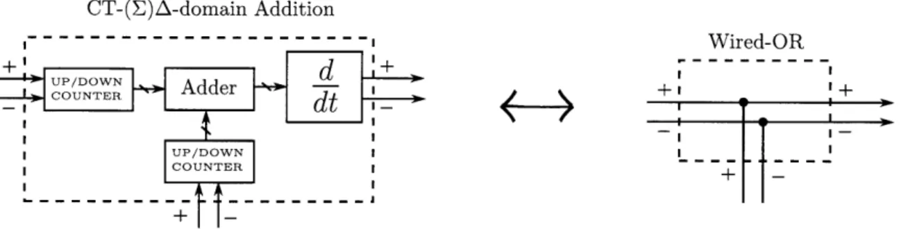
The three linear time-invariant (LTI) operations-addition, constant multiplication, and delay-are straight-forward in the CT-A and I&F pulse domain. Because these operations are LTI, CT-A and I&F processing elements are identical. Modules that perform these operations take in positive or negative pulses and output