Equilibrium modeling of the Beach Profile on a Macrotidal Embayed Beach

(1)

HAL Id: hal-01580926

https://hal.archives-ouvertes.fr/hal-01580926

Submitted on 3 Sep 2017

HAL is a multi-disciplinary open access

archive for the deposit and dissemination of

sci-entific research documents, whether they are

pub-lished or not. The documents may come from

teaching and research institutions in France or

abroad, or from public or private research centers.

L’archive ouverte pluridisciplinaire HAL, est

destinée au dépôt et à la diffusion de documents

scientifiques de niveau recherche, publiés ou non,

émanant des établissements d’enseignement et de

recherche français ou étrangers, des laboratoires

publics ou privés.

Equilibrium modeling of the Beach Profile on a

Macrotidal Embayed Beach

Clara Lemos, France Floc’h, Marissa Yates, Nicolas Le Dantec, Vincent

Marieu, Klervi Hamon, Véronique Cuq, Serge Suanez, Christophe Delacourt

To cite this version:

Clara Lemos, France Floc’h, Marissa Yates, Nicolas Le Dantec, Vincent Marieu, et al.. Equilibrium

modeling of the Beach Profile on a Macrotidal Embayed Beach. Coastal Dynamics 2017, Jun 2017,

Helsingor, Denmark. pp.760-771. �hal-01580926�

(2)

Equilibrium modeling of the Beach Profile on a Macrotidal Embayed Beach

Clara Lemos1, France Floc’h1, Marissa Yates2, Nicolas Le Dantec1,,3, Vincent Marieu4, Klervi Hamon1, Véronique Cuq5, Serge Suanez5, Christophe Delacourt1

Abstract

Predicting the pluriannual variability of shoreline position in response to hydrodynamic forcing (waves and tides) is of primordial interest scientists, engineers, and beach managers. 11-year time series of monthly profile beach survey and hourly incident wave conditions are analyzed on a macrotidal sandy embayed beach in Brittany (France). An equilibrium model is applied to study the variation of the beach profile position over the whole intertidal zone as a function of the energy wave, wave power and water level. The predictive ability of the equilibrium model is around 60% in the upper intertidal zone but decreases with decreasing elevation in the lower intertidal zone. The predicted result on the lower part taking into account of the still water level is not improved, but the erosion and accretion parameters are more reliable, according to the physical processes and could be compared to other study sites.

Key words: equilibrium model, macrotidal, intertidal profile, shoreline, cross-shore processes, waves.

1. Introduction

Predicting the temporal variability of shoreline position in response to hydrodynamic forcing (waves and tides) is of primordial interest for coastal scientists, engineers, and beach managers. Shoreline position changes along sandy coast vary over a wide range of temporal and spatial scales in response to a wide range of physical processes (Stive et al., 2002; Masselink et al., 2016). On short timescales ranging from hours to days to years, single storms causing variations in the wave energy arriving at the coast may be the dominant processes impacting shoreline changes and sediment transport processes. On most open coasts, alongshore processes typically have more important role on longer timescale than cross-shore processes and do not dominate the annual shoreline variability (e.g. Davidson and Turner, 2009; Yates et al., 2009;

Hansen and Barnard, 2010; Castelle et al., 2014). Understanding beach profile response to energetic waves

and subsequent calms periods is crucial as rising seas encroach on coastal infrastructure and climate change is expected to modify storm frequency and intensity (Stocker et al., 2013; Ludka et al., 2015).

Beach profile response to hydrodynamic forcing has long been studied, Brunn (1954) and Dean (1977, 1991) developed empirical functions to describe observed equilibrium profile shapes. Furthermore, Wright and Short (1985) showed that the state of the beach is determined by recent history of both the wave field and the morphology. These concepts have been used in a variety of empirical models to study changes in shoreline position on timescales of days to years on sandy beaches dominated by cross-shore processes

(e.g. Miller and Dean, 2004; Davidson and Turner, 2009; Yates et al., 2009; Davidson et al., 2010; Yates et

al., 2011; Davidson et al., 2013; Castelle et al., 2014; Ludka et al., 2015). These models simulate shoreline variations as a function of wave conditions and the previous position of the shoreline. Yet, the shoreline

1_{Géoscience Océan - UMR 6538, Université de Bretagne Occidentale, Institut Universitaire Européen de la Mer, rue} Dumont d’Urville, 29280 Plouzané, France, France.floch@univ-brest.fr

2

Saint-Venant Laboraty for Hydraulics (ENPC,EDF, R&D, CEREMA), Université Paris-Est, Centre d’étude et d’expertise sur les Risques, l’Environnement, la Mobilité et l’Aménagement, CEREMA, Margny-Les-Campagne, France.

3

CREMA -Centre d’étude et d’expertise sur les Risques, l’Environnement, la Mobilité et l’Aménagement, DTecEMF, 29280 - Pluzané, France.

4

EPOC - OASU, URM 5805, Site de Talence, Université Bordeaux 1, France. 5

Géomer - LETG UMR 6554, Université de Bretagne Occidentale, Institut Universitaire de la Mer, rue Dumont d’Urville, 29280 - Plouzané, France.

(3)

Coastal Dynamics 2017 Paper No. 057

position models need extensive historical observations and are calibrated for each specific site (Yates et al.,

2009; Splinter et al., 2014; Ludka et al., 2015). Castelle et al. (2014) suggested that equilibrium shoreline

models can be extended and applied to a range of altitudes in the intertidal one. The model developed by Yates et al. (2009) is able to predict shoreline position changes with an efficiency of approximately 80% (Yates et al., 2009; Ludka et al., 2015) on microtidal beaches. On a recent extension to mesotidal beaches, a similar model performs with approximately 65% efficiency (Castelle et al., 2014).

In macrotidal environments, wave conditions and hydrodynamic processes vary throughout the width of intertidal zone. At low tide, there is high dissipation over the shelf, and the wave energy reaching the beach may be significantly lower than the offshore wave energy. This dissipation is less important at high tide, and the energy reaching to upper part of the beach is comparable to the offshore wave energy. Many observations show that morphological changes occur along entire beach profile, but the change are very inhomogeneous along cross-shore profile, especially on Low Tide Terrace (LTT) beaches (Almeida et al., 2017). Empirical modes have been proven to predict well the variations observed on the upper part of the beach (Yates et al., 2009), with reduced predictive skills on the lower beach. This paper investigates the ability of an empirical model to predict pluriannual morphodynamics of the intertidal zone in a macrotidal environment. One important question is how to associate the model free parameters to physical processes (e.g. erosion and accretion rates) when at same altitudes, wave energy actually impacts the zone only 5% of the time whereas changes are simulated 100% of the time in the model. This study investigates how to take into account the effects of changing eater levels (e.g. the tidal effects) by defining a vertical range bounding a strip of the beach within which the wave energy may cause changes in the cross-shore position at any altitude.

This study focuses on a macrotidal embayed beach (Porsmilin beach), located in western Britanny (France) on the Iroise sea coastline (Figure 1 a, b). Porsmilin beach has cliffs at both ends and bedrock in the intertidal zone. The primarily cross-shore dominant morphological processes make this sandy beach an ideal site to study cross-shore variation along the intertidal profile using an empirical equilibrium model forced by the incident wave energy or wave power. Because of the large tidal range at Porsmilin beach, the evolution of the upper and lower parts of the intertidal profile varies significantly for the same incident wave conditions. Thus, it is important to test the predictive ability of the model when the tide level is taken into account. Here, the approach chosen for this purpose is to define for each step during the model calculation a condition that is used to determine whether the empirical model takes into account the impacts of the incident waves. That condition is established using the difference between the beach elevation contour simulated during the model run and the still water level predicted taking into account tide only. When the elevation contour can no longer be reached by water (including the effects of runup) or when the water becomes very deep, the impacts of incident waves are considered negligible, and cross-shore position is not modified in the model.

First, the study site and morphological and hydrodynamical data are described (section 2). Then, the extension of an equilibrium shoreline model (Yates et al., 2009) attempted to take into account the effect of instantaneous water level is described, and the results are presented when the model is forced either with the wave energy or wave power. Finally, the results on the performance of the model tested under the various hypotheses are discussed and compared to other studies (section 5).

2. Study Site and data 2.1.Study site

Porsmilin beach is an embayed barrier beach flanked by cliffs to the East and West, and backed by colmated brackish water marshes to the North. The intertidal zone is 200 m wide and 200 m long (Figure 2 a) and the sediment median grain size (d50) is 320 µ m. It is bounded by headlands and bedrock, extends offshore and obstructing the alongshore sand transport generated in the surf zone and allowing incident wave from the SW only. The alongshore sediment flux is assumed negligible since the shoreline does not exhibit rotation behavior (Floc’h et al., 2016). According to the Masselink and Short (1993) classification, Porsmilin beach is a Low Tide Terrace beach (Dehouck et al., 2009

(4)

Due to its orientation in the Iroise Sea, Porsmilin beach is mainly impacted by southwest waves that have peak periods between 8 s and 10 s. The Iroise Sea is a highly energetic wave dominated environment, and the return period of significant wave heights of 11.3 m and 14.5 m (in 110 m water depth at the West of France) are 1 and 10 years (Dehouck et al., 2009). The tides are semi-diurnal and symmetric with a mean spring tidal range of 5.7 m and a mean spring tidal current of 0.4 m/s in Bertheaume Bay (Shom, 1994). Between 2002 and 2014, the mean significant height was 0.76 m and the seasonal means in autumn, winter and spring were 0.7 m, 1.08 m and 0.7 m respectively. However, along this rocky coastline, wave propagation is considerably affected by refraction and diffraction processes generated by the large continental shelf, headlands, shoals and islands located offshore of the beach (Ouessant Island, Molene archipielago). Hence, the oceanic swells that reach the shoreline have a quasi normal incident angle and are already highly dissipated, resulting in moderate energy conditions at Porsmilin beach.

2.2.Beach profiles surveys

Monthly cross-shore surveys were completed from January 2003 to January 2014 (Figure 2 b) with a Differential Global Positioning System (DGPS) RTK (referenced to the topographic French datum IGN69). During this period, 174 profiles of sand levels were measured along a cross-shore transects with 1 m horizontal resolution. For each profile, the data is interpolated to a 0.1 m horizontal resolution between 0 m and 4.4 m, as well as at -1 m, -0.6 m and -0.2 m. Depending on the tide level, each cross-shore profile has a different length, and 172 profiles extended vertically from 0 m to 4.1 m (IGN69). Thus, to calibrate the empirical model, 172 profiles were used from 0 to 0.3 m, 173 from 0.4 to 0.8 m and 174 from 0.9 to 4.1 m.

Figure 1: a) and b) Maps of NW France showing the location the Porsmilin beach.

a) _b)

Figure 2: a) Planview of the morphological characteristics of the Porsmilin beach. b) Cross-shore profiles at

Porsmilin from January 2003 to January 2014, indicating mean beach profile (red profile) and Mean High Water Spring (MHWS) level, Mean High Water Neap (MHWN) level and Mean Water (MW) level.

(5)

Figure 4: a) Scatter diagram of the significant wave height modèle WWIII (HswwIII) and significant wave height ADCP (HsADCP) and peaks period WWIII (TpwwIII), the solid red line is the regression linear giving y = 1.5920x+0.1548. b) Scatter diagram of the significant wave height model WWIII (HswwIII) and peak period

model WWIII (TpwwIII), the solid red line is the regression linear giving y=0.5593x-3.6545.

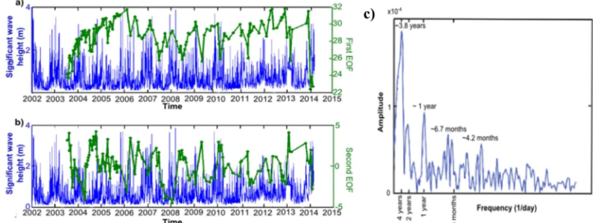
An EOF (Empirical Orthogonal functions) analysis of the detrended timeseries demonstrated that two principal modes describe 90% of the cross-shore variability (Hamon, 2014). The first EOF represents the variations on the upper part of the beach, with a seasonal berm appearing at the MHWS level during summer, persisting through autumn, and then disappearing progressively in winter and spring (Figure 3 a). This mode is correlated with Hs all over time series. The second EOF represents the variations along the profile between the MNHW level down to the lower part of the beach (Figure 3 b). This mode is by definition in independent from the first EOF and is thus not correlated with Hs. The spectrum of its temporary amplitude shows a peak period of 3.8 years (Figure 3 c) and only a small seasonal component. This period does not seem to be related to the wave climate or other global climate factors, and more investigations are needed to fully understand the beach dynamics on these timescales.

2.3.Wave and tide data

The empirical model computes the current shore position from the wave forcing and previous cross-shore position. Hourly wave conditions in 20 m water depth from the numerical model WaveWatchIII (WWIII) are used from January 2002 to January 2014 (Norgas-UG configuration at the grid point 4º40,66’W, 48º33’ N, Tolman, 1991). The accuracy of wave forcing is compared with the in-situ measurements collected by acoustic Doppler Current Profiler deployed during two campaigns (25 November to 31 December 2013, and 24 September to 8 November 2014) at the grid point 4º40.80’W, 48º20.80’N. The linear regression between the modelled (HswwIII) and measured (HsADCP) wave heights R2 = 0.88 (Figure 4 a).

However, the peak period (Tp) and significant wave height (Hs) from WWIII are not linearly related (Figure 4 b). Therefore, in the following, both wave energy and wave power (taking into the effects of the

c)

Figure 3: Empirical Orthogonal Functions (EOF) analyses from 2002 to 2014. (a) Correlation between significant

(6)

wave period) will be tested to force the model. The peak period (Tp) data is only available between 1 January 2008 and 1 January 2014, which correspond to 66 beach profiles. Finally, hourly estimates of the tide level (2002 to 2014) from the SHOM (National Hydrographic Service) are used from the grid point 4º49.48’W, 48º38.29’N.

3. Method

3.1. Equilibrium model

An equilibrium shoreline model (Yates et al., 2009; Castelle et al., 2014) is applied at discrete elevations along the intertidal beach profile, ranging from 0 to 4.1 m (every 0.1 m) as well as at -1 m, -0.6 m and -0.2 m. The model simulates temporal changes of the cross-shore position of each elevation using an equilibrium approach. The beach evolves towards equilibrium as a function of both the intensity of the wave forcing (e.g. wave energy or power) and the disequilibrium between the current and equilibrium conditions (defined as a function of the current contour position), which causes the beach to erode or accrete. In this study, the model developed by Yates et al. (2009) is used for predicting the change in the cross-shore position (dS/dt), witch depends on both the wave energy (E) and the wave energy disequilibrium (∆E):

dS/dt= C± E1/2 ∆E (1) for ∆E = E – Eeq (S) , (2)

where C± are rate coefficient for accretion (C+ for ∆E<0) and erosion (C- for ∆E> 0). The equilibrium wave energy (Eeq) is defined as a linear function of the cross-shore position Eeq (S) =aS+b. In this model, the cross-shore position change rate depends on wave energy, but the cross-shore position does not depend on wave direction or alongshore gradient in waves or currents (Yates et al., 2011). The model developed by Yates et al. (2009) presents four free parameters: a and b determining the equilibrium energy for each cross-shore position, and C± the accretion and erosion coefficients. Here, following Castelle et al. (2014), a fifth free parameter, d, is added to reduce the dependence of the model on the initial cross-shore position. This parameter represents a deviation of the mean position, that is used to initiate the timeserie. Simulated annealing (Barth and Wunsch, 1990) allows to obtain the five free parameters of the model decreasing the root-mean-squared error (RMSE) between the model and observations. The number of the interactions is 700000 with a minimum number of loops of 200. In addition, a range of values is set the different parameters: -5 / 0 m2/m for a, 0 / 2 m2 for b, -12 / 0 mhr-1/m3 for accretion and erosion coefficients, and -30 / 30 m for d.

First, the model is tested to evaluate the effects the wave energy on the variation the cross-shore position. Then, the wave power is used to force the model since the mean period has been shown to play an important role in the beach morphodynamics at Porsmilin beach (Floc’h et al., 2016).

3.2. Equilibrium model taking into account the water level

To take into account the effect of the water level, two hypothesis are made. The first hypothesis states that when the water level is too far below the elevation Z0 (Figure 5 a), it is obvious that the incident wave field does not impact the contour position. The second hypothesis is less obvious: the erosion and accretion processes outside the surf zone are assumed to have less impact than those in the swash zone, and thus, the cross-shore variation of the contours is assumed small when the simulated elevation contour is no longer in the surf/swash zone. Thus, the cross-shore position at a given elevation contour will not change in the model if its altitude is: (1) above the maximum runup observed on the beach (about 1 m the considered site), or (2) under the wave height (about 1.5 m), which is used to define the lower limit including the wave breaking zone. A vertical threshold L (see Figure 5.) is defined to determine the times periods during which the incident wave field causes significant sediment transport around the given elevation contour. L is assumed symmetric about the water level Z0 for simplicity (maximum runup as upper limit, surf zone limit as lower limit). In the model, the difference between the simulated elevation contour (Z0, Figure 5) and the instantaneous still water level (hourly tidal predictions obtained from SHOM) is calculated and compared

(7)

to this threshold. If the absolute value of this difference is greater than L, then the simulated shoreline position is not modified (blue zones, Figure 5 b). A series of sensitivity test are conducted to evaluate the impact of this threshold L, with L=0.5 m, 1 m, 1.5 m, 2 m, 2.5 m, 3 m. In this study, for each simulation, the model skill was evaluated with the R-squared coefficient (of determination) denoted R2, and the root-mean-squared error (RMSE) between modelled and observed cross-shore position.

4. Results

4.1.Yates et al. (2009) empirical model application

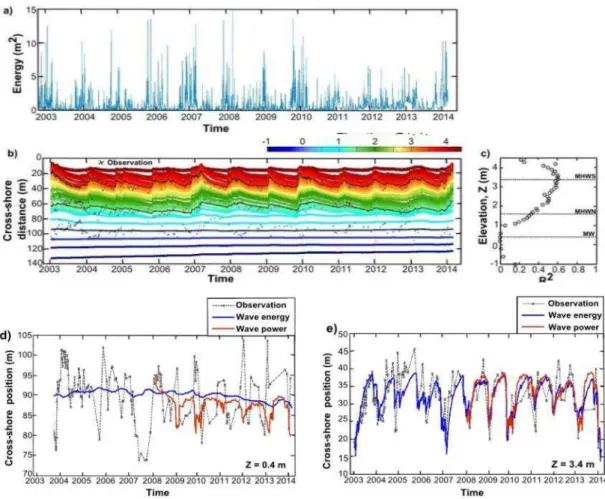
During the investigated period, the wave energy at Porsmilin beach varies seasonally. From 2003 to 2014, the winters of 2006, 2008 and 2010 are the most energetic (Figure 6 a). The model reproduces well the variation of the cross-shore position at seasonal and weekly scales on the upper part of the beach down to an elevation (Z) of approximately 2.2 m with an R2 > 0.5 (Figure 6 c and Figure 9 a) The best predictive ability of the model, with R2=0.6, is observed at 3.4 m elevation (MHWS). The predictive ability is the same if the model is forced with wave wave energy or wave power, and it decrease with the elevation in all the test performed (Figure 6 c) show that the predictive ability of the model decreases with the elevation in all the tests performed. Below the MHWN level, the predictive ability decreases considerably (R2 <0.3). On the upper part of the beach, the model is able to reproduce well the observed erosion trends, including the significant periods of erosion in the winters of 2006/2007 and 2013/2014 (Figure 6 a, b). The performance of the model decrease during periods of accretion, when the contour position change rates are smaller, but the cumulative accretion is still important. Below the Mean Water (MW) level, the model simulations forced with the wave energy show no significant variations (light and dark blue curves, Figure. 6 b), even though the observations show an amplitude of variability comparable to that of the upper part of the beach. When the model is instead forced with wave power, temporal variations are obtained on the lower part of the beach, but the correlation remains low (Figure 9 a).

The results of the model simulations are not significantly improved when forced by the wave power instead of the wave energy (e.g. elevations contours 0.4 m and 3.4 m, Figure 6 d, e). The cross-shore variations in the 0.4 m contour are not reproduced when the model is forced with wave energy. By using the wave power, simulated cross-shore changes are observed during periods of erosion, but the model skill is not increase significantly (Figure 6 d). For the 3.4 m contour, the empirical model is able reproduce the seasonal variability of the cross-shore position (Figure 6 e), using wave energy or wave power.

Figure 5: Diagram showing how the water level is taken into account in the equilibrium model (a) beach profile with

the selected elevation contour Z0 and modeling threshold L, (b) tide level determining the times periods (red) when the wave forcing the cross-shore position.

(8)

The free parameters a is between -0.1 m/m2 and 0 m/m2 when the model is forced with the wave energy (Figure 7 a). The free parameter b presents values around 0 m2 for the elevations between -1 m to 3.2 m and the elevations between 3.3 m to 4.4 m the values is around 1.2 m (Figure 7 b)). The erosion (C-) and accretion (C+) coefficients are in the range of -0.4 mhr-1/m3 to 0 mhr-1/m3and -0.2 mhr-1/m3 to 0 mhr-1/m3 respectively (Figure 7 c, d). These two change rate coefficients tend to increase with increasing elevation until 3.6 m before decreasing again. In the lowest part of beach, for the elevation contours -1 m, 0.2 m, 0.4 m and 0.6 m the accretion free parameter (C+) present the values around -12 mhr-1/m3 showing that the model has some limitations in representing accurately to accretion processes. When model is forced with wave power, the free parameter a and coefficient erosion show small variations (Figure 7 a, c). The erosion coefficient is aroud 0 mhr-1/m3, but the accretion coefficient ranges from -2 mhr-1/m3 and 0 mhr-1/m3.

Figure 6: Wave conditions, predictive ability of the model, and R2 values for ranging from -1 to 4.4 m for wave

energy (m2) (2003-2014) (a), (b), and (c). The predictive ability of the model in (b) compares the observed (crosses) and equilibrium model simulation (colored lines) cross-shore contour positions. Cross-shore observation

and the model simulation when the model is forced with the wave energy and wave power. (d) Elevation 0.4 m.

(9)

Figure 8: Predictive ability of the model as a function of the water level, between 2003 and 2014. (a) Observed

(crosses) and simulated (colored lines) cross-shore contour position equilibrium model as a function of the water level (b) R2 value for contour ranging from 0 to 4.1 m.

4.2.Effects of water level

The model is able to predict seasonal cross-shore variations the model takes into account the effects of the water level for all tested threshold (L). For threshold of L=3 m (Figure 8), the model predicts well the variations in the upper part of the beach, but its predictive ability decreases with elevation. In addition, the highest predictive capacity is still around 3.4 m, with values R2 above 06 (Figure 8 b). In the lower part of the beach, the R2 eventually reaching nearly 0 (Figure 8 b). Even if the model only simulates cross-shore changes in the contour elevations for limited periods during a tidal cycle, it is still of reproducing observed erosion and accretion trends on timescales of weeks to months.

When taking account the water level, the determination coefficient R2 does not change significantly on the upper part of the beach (MHWS) even if the cross-shore position rarely changes because the water reaches this altitude only during spring tides (for a few hours a couple of days per month). The R2 values for the model forced with thresholds are slightly higher for elevation between 1 m and 4.1 m (Figure 9 a). When the model is forced with the wave power, the coefficient R2 values are lower between 1 m to 2.5 m, but this difference may be caused by the difference in the simulation period.

Figure 7: Optimal free parameters for each elevation contour when the model is forced with wave

energy (a, b) and wave power (e,h): (a,e) Equilibrium slope a, (b, f) Equilibrium wave energy intercept b, (c,g) accretion coefficient C+, and (d, h) erosion coefficient C-.

Figure 9: (a) Coefficient of determination (R2) of the simulation as a function of the wave energy and, wave power for each value of threshold (L). (b) Percentage of hours of waves causing cross-shore contour changes as

(10)

The percentage of wave conditions causing contour changes for lower elevations, especially for larger values of L. For elevation between 0 m and 1 m, for L=3 m, the this percentage is almost 100%, but for the same threshold for an elevation between 3.5 and 4 m, the percentage decrease to 80 % (Figure 9).When taking into account the effects of the water level, the free parameters a and b are very similar that those of the wave energy only model (Figure 7 a, b and Figure 10 a, b). The most important differences appear in the erosion and accretion coefficients, as expected (Figure 7 c, d and Figure 10 c, d). These coefficients are larger for higher elevations (Figure 10 c, d), and for smaller values of threshold L.

5. Discussion

The efficiency of the empirical model used in this study is 60% around Mean High Water Spring level (MHWS) on a macrotidal beach. This study shows that, the empirical model developed by Yates et al. (2009) and Castelle et al. (2014) is a robust model able to predict contour elevation variations in different tidal regimes, on the upper part of the beach. This model is able to predict the variation of the shoreline on the microtidal beach with a higher efficiency of 90% (Yates et al., 2009; Yates et al., 2011; Ludka et al., 2015) and on mesotidal beach with an efficiency around 70 % (Castelle et al., 2014). The models predictive abilities (estimated from the R2 coefficient) is similar whether the model is forced by wave energy or, wave power, and when the model takes into account the effects of the water level.

5.1. Wave power

The wave power was tested in the model instead of the energy to be able to simulate the cross-shore variations observed for elevation contours below the MW level. These variations have amplitude comparable to those observed on the upper part of the beach. However, changes on the upper and lower part of the beach are not correlated to each other, and the changes observed on the lower part of the beach do not show the same seasonal variability as the wave height, as seen in the EOF analysis. By forcing the model with the wave power or by taking into account the effects of the water level, a better fit is expected on the lower part of the beach.

The wave power allows the empirical model to converge to a solution with amplitude of cross-shore position variation comparable to the observations on the lower part of the beach. As a reminder, the model with wave energy shows no variation at all in the lower part of the beach. Nevertheless, the simulated variations appear out of phase with the observed variations, leading to poor R2 values. Thus, the wave period has an impact on the lower part of the beach but leads to an opposite effect as that observed. However, this does suggest that the period has an impact on the sediment transport between the upper and lower parts of the beach. This may be expected is one considers that the erosion of the upper part of the beach leading to a transport to the lower part. Since the wave power is more important at high tide than at

Figure 10: Optimal free parameters as function of the elevation when the model takes into account the effects of

the water level: (a) equilibrium slope a,. (b) intercept the equilibrium wave energy b,. (c) accretion coefficient C+, and (d) erosion coefficient C-_.

(11)

Figure 11: Optimal free parameters on the Truc Vert beach ( Castelle et al. 2014) and Porsmilin beach: (a) equilibrium slope a,. (b) intercept the equilibrium wave energy b,. (c) accretion coefficient C+, and (d) erosion

coefficient C-.

low tide (less dissipation over the self), the erosion in the upper part could lead to an accretion in the lower part. However, one must note that the cross-shore elevation contours on the upper part of the beach are not correlated (Figure 12) and thus the sediment exchanges between the upper and lower part of the beach are not as simple suggested.

5.2. Water level

Since the water level has an important impact on the amount of wave reaching each contour level, the model simulations taking into account the water level should lead to a more realistic interpretation of the results. The empirical model converges to a solution that is as good as the model without the water level adjustment, and the coefficients a and b remain the same since they are independent of the duration of the wave impact. However, the coefficients C+ and C- change depending on the water level threshold L since they rate coefficients that depend strongly on the duration of wave impact. On the upper part of the beach, the model does not simulate contour elevation changes during the largest percentage of time, leading to the largest increases in these coefficients, as would be expected.

5.3. Comparison with other study sites

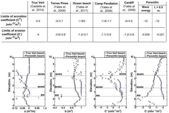
The free parameters the equilibrium model show the difference between the different tests performed. The limits on the accretion C+ and erosion C- coefficients are important when the model depends on the water level with threshold (L) in the range 0.5-1 m, in particular. When the model takes into account the effects of the water level, the accretion coefficients are similar to those the shown on other beaches (for example the rate around of -4 mhr-1/m3 at Tuc Vert beach (Castelle et al., 2014) and -3 mhr-1/m3 at Torres Pines (Yates et al., 2009)) (Table 1 and Figure 11). The erosion coefficient is very small compared other beaches, but the rate is similar to that estimated at Ocean beach (Yates et al., 2011) (Table 1). One must note the differences between sites in the erosion and accretion rate coefficients may be expected owing to differences in sand grain size. These results show that taking into account the water level may allow for a more physical interpretation of the erosion and accretion rate coefficients that are likely closer to the true values.

Table 1: accretion and erosion coefficient at the different study beach (Yates et al., 2009; Yates et

(12)

5.4. Limitations of the model

The presented equilibrium model is a simple approach that depends on a limited number of free parameters. The model is limited by the assumption that the equilibrium wave energy is a linear function of the contour position, whereas as for low energy thet more likely tend to zero but never reach zero. Considering such an equilibrium function may improve the accretion predictions.

It is also not trivial task to determine the best value for the water level threshold L (and this the most realistic accretion and erosion coefficients) since the R2 value does not vary significantly for different values of L, and the hypothesis that L is symmetric about the simulated elevation contour may not be valid. The main issue met here is the boundary value 0 for the parameter a (slope of the equilibrium model) in order to maintain erosion when energy increase. Actually, on the lower part of the beach, accretion occurs when the upper part erodes (Figure 12). The lower part of the beach behaves oppositely to the upper part. The main improvement on the lower part of the beach comes from the extended range of parameter allowing increasing accretion when wave energy increases. Actually, this allows to simulate the sediment transfer occurring between the upper part and the lower part of the beach. However, this is not enough to explain the pluriannual variability observed on the lower part of the beach.

Conclusion

This study attempts to improve predictions of shoreline evolution on macrotidal beaches in response to storms and multiannual timescales to be able to provide crucial information to coastal planners. The presented model extends the Yates et al. (2009) model to be a robust, simple, and efficient empirical model that allows reproducing the contour elevation variation on beaches with a different tidal range. The model presents a strong predictive ability on the upper part of the beach where the sedimentary dynamics depends on the energy of the waves, but the model performance decreases on the lower part of the beach where the relationship between the sediment dynamics and the wave characteristics is more complex (and depends on other physical parameters such as the wave period, with a pluriannual cycle highlighted).

The extension of the model to take into account the effects of the water level does not significantly improve model’s predictive ability. However, this extension does improve the physical interpretation of the estimated erosion and accretion coefficients, and more work needs to be done on other macrotidal beaches to improve the estimates of these parameters and to evaluate the importance of the sediment grain size. Thus, it is probably necessary to investigate and apply the generalized model presented by Splinter et al. (2014) that presents a predictive capacity around 80 % in the twelve beaches used allowing to obtain information of the possible limits in the macrotidal environments.

Acknowledgements

This work was supported by the Labex-MER funded by the Agence Nationale de la Recherche under the program « Investissements d'avenir » with the reference ANR-10-LABX-19-01, the lab Domaines Océaniques UMR6538 and the Pôle Image of IUEM. The long term measurements were successively supported by the ANR COCORISCO (2010-CEPL-001-01), the SOERE trait de côte and the NSO Dynalit.

(13)

References

Almeida L. P., Almar R., Marchesiello P., Blenkinsopp C., Martins K, Sénéchal N., Floc'h F., Bergsma E., Benshila R., Caulet C., Biausque M., Duong T. H., Le Thanh B., Nguyen T. V. (2017). Tide control on the swash dynamics of a steep beach with low-tide terrace. Marine Geology, accepted with minor revisions.

Barth, N., and Wunsch, C. (1990). Oceanographic experiment design by simulated annealing. Journal of Physical Oceanography, 20: 1249-1263.

Bruun, P.1954. Coastal erosion and developpement of beach profiles. Thecnical Memorandum No. 44, U.S. Army Corps of Engineers. Washington.

Castelle, B., Marieu, V., Bujan, S., Ferreira, S., Parisot, J-P., Capo, S., Sénéchal, N., Chouzenoux, T., 2014. Equilibrium shoreline modelling of a high-energy meso-macrotidal multiple-barred beach. Marine Geology, 347: 85-94. Davidson, M.A. and Turner, I.L., 2009. A behavioral template seasonal to multi-year shoreline change. Coastal

Engineering, 57:620-629.

Davidson, M.A., Lewis, R.P., Turner, I.L., 2010. Forecasting seasonal to multi-year shoreline change. Coastal Engineering, 57: 620-629.

Davidson, M.A., Splinter, K.D., Turner, I.L., 2013. A simple equilibrium model for predicting shoreline change. Coastal Engineering, 73, 191-202.

Dean, R.G., 1977. Equilibrium beach profiles: U.S. Atlantic and Gilf Coasts. Technical Report No.12, Departement of Civil Engineering, University of Delaware.

Dean, R.G., 1991. Equilibrium beaches profiles : Characteristic and applications. Journal of Coastal Research, 7(1) :53-84.

Dehouck, A., Dupuis, H., Sénéchal, N., 2009. Pocket beach hydrodynamics : The example of four macrotidal beaches, Brittany, France. Marine Geology, 2006: 1-17.

Floc’h, F., Le Dantec, N., Lemos, C., Cancouët, R., Sous, D., Petitjean, L., Bouchette, F., Ardhuin, F., Suanez, S., Delacourt, C., 2016. Morphological Reponse of a Macrotidal Embayed Besach, Porsmilin, France. Journal of Coastal Research, Special, 75: 373-377.

Hamon, K., 2014. Etude de la morphodtnamique et du profil d’équilibre d’une plage de poche macrotidale. Master Report, University Bretagne Occidentale, 61.

Hansen, J.E., Barnard, P.L., 2010. Sub-weekly to interannual variability of a high-energy shoreline. Coastal Engineering, 57: 959-972.

Ludka, B.C., Guza, R.T., O’Relly, C., Yates, M.L., 2015. Field evidence of beach profile evolution toward equilibrium. Journal of physical Research; Oceans, 120: 7574-7597.

Masselink, G., and Short, A.D., 1993. The effect of tide range on morphodynamics and morphology: A conceptual beach model. Journal Coastal Research, 9(3): 785-800.

Masselink, G., Castelle, B., Scott, T., Dodet, G., Floc’h, F., Jackson, D., 2016. Extreme wave activity during 2013/14 winter morphological impacts along Atlantic coast of Europe. Geophysical Research Letters, 43: 2135 – 2143. Miller, J.K. and Dean, R.G., 2004. A simple new shoreline change model. Coastal Engineering, 51, 531-556. SHOM, 1994. Courants de marée de la côte ouest de Bretagne de Goulven à Penmarc’h.

Splinter, K.D., Turner, I.L., Davidson, M.A., Barnard, P., Castelle, B., Oltman-Shay, J., 2014. A generalized equilibrium model for predicting daily to unterannual shoreline response. Journal of Geophysical Research: Earth Surface, 119: 1936-1958.

Stive, M.F.F., Aarninkhof, S.D.J., Hamm, L., Hanson, H., Larson, M., Wijnberg, K.M., Nicholls, R.J., Capobianco, M., 2002. Variability of shore and shoreline evolution. Coastal Engineering, 47: 211-235.

Stocker, T.F., Qin,D., Plattner, G.K., Tignor, M., Allen, S.K., Boschung, J., Nauels, A., Xia, Y., Bex, V., Midgley, P.M., 2013. Climate Change 2013: The physical Science Basis. Contribution of working group I to the fifth assessment report climate change. Cambridge University Press, Cambridge, U.K.

Tolman, H.L., (1991). A third-generation model for wind waves on slowly varying, unsteady, and inhomogeneous depths ans curents. Journal of Physical Oceanography, 21: 783-797.

Wright, L.D., Short, A.D., Green M.O., 1985. Short-term changes in the morphodynamics states of beaches and surf zones: An empirical predictive model. Marine Geology, 62: 339-364.

Yates, M.L., Guza, R.T., O’Reilly, W.C., 2009. Equilibrium shoreline response: Observations and modeling. Journal of Geophysical Research, 114 (C09014).

Yates, M.L., Guza, R.T., O’Reilly, W.C., Hansen, J.E., Barnard, P.L, 2011. Equilibrium shoreline response of a high wave energy beach. Journal of Geophysycal Research, 116(C04014).