HAL Id: hal-01872332
https://hal.archives-ouvertes.fr/hal-01872332
Submitted on 12 Sep 2018
HAL is a multi-disciplinary open access
archive for the deposit and dissemination of
sci-entific research documents, whether they are
pub-lished or not. The documents may come from
teaching and research institutions in France or
abroad, or from public or private research centers.
L’archive ouverte pluridisciplinaire HAL, est
destinée au dépôt et à la diffusion de documents
scientifiques de niveau recherche, publiés ou non,
émanant des établissements d’enseignement et de
recherche français ou étrangers, des laboratoires
publics ou privés.
Study of the thrust–drag balance with a swimming
robotic fish
Florence Gibouin, Christophe Raufaste, Yann Bouret, Médéric Argentina
To cite this version:
Florence Gibouin, Christophe Raufaste, Yann Bouret, Médéric Argentina. Study of the thrust–drag
balance with a swimming robotic fish. Physics of Fluids, American Institute of Physics, 2018, 30 (9),
�10.1063/1.5043137�. �hal-01872332�
Study of the thrust–drag balance with a swimming robotic fish
Florence Gibouin, Christophe Raufaste, Yann Bouret, and Médéric ArgentinaCitation: Physics of Fluids 30, 091901 (2018); doi: 10.1063/1.5043137 View online: https://doi.org/10.1063/1.5043137
View Table of Contents: http://aip.scitation.org/toc/phf/30/9
PHYSICS OF FLUIDS 30, 091901 (2018)
Study of the thrust–drag balance with a swimming robotic fish
Florence Gibouin,1Christophe Raufaste,1Yann Bouret,1and M´ed´eric Argentina1,2,a)1Universit´e Cˆote d’Azur, CNRS, Institut de Physique de Nice, 06100 Nice, France 2Institut Universitaire de France, 75005 Paris, France
(Received 6 June 2018; accepted 22 August 2018; published online 11 September 2018)
A robotic fish is used to test the validity of a simplification made in the context of fish locomotion. With this artificial aquatic swimmer, we verify that the momentum equation results from a simple balance between a thrust and a drag that can be treated independently in the small amplitude regime. The thrust produced by the flexible robot is proportional to A2f2, where A and f are the respective tail-beat amplitude and oscillation frequency, irrespective of whether or not f coincides with the resonant frequency of the fish. The drag is proportional to U2
0, where U0is the swimming velocity. These three physical quantities set the value of the Strouhal number in this regime. For larger amplitudes, we found that the drag coefficient is not constant but increases quadratically with the fin amplitude. As a consequence, the achieved locomotion velocity decreases, or the Strouhal number increases, as a function of the fin amplitude. Published by AIP Publishing.https://doi.org/10.1063/1.5043137
I. INTRODUCTION
Most macroscopic swimmers undulate their bodies to gen-erate a net thrust and propel themselves. Using Theodorsen’s aerodynamics of rigid wings,1 in 1936, Garrick studied self-propelled vibrating foils.2 Since then, flapping foils have been efficient experimental devices to model fish propulsive motion.3–5This approach has resulted in showing that an opti-mum for propulsion is achieved through a combination of heave and pitch with a phase difference of 90◦.6,7
Concentrating on the theoretical aspects of fish propul-sion, Lighthill established the slender-body theory for deformable bodies to make thrust calculations.8,9 The effect
of appendage flexibility has since been investigated in pitch-ing movements,10,11heaving motions,12–16and a mix of them
both17,18 or by confining the swimmer in the vicinity of a wall.19 For all the studies mentioned, the thrust is notably enhanced when the foils are forced near their resonant fre-quencies.20These are associated with the eigenmodes of the system comprised of the plate-like foil coupled to its surround-ing fluid. For elastic plates forced by an oscillatsurround-ing torque distribution, the highest velocities are also observed near the resonant frequency forcing.21
Data collected from natural swimmers show that the swimming characteristics in the turbulent regime, i.e., a Reynolds number Re larger than 3000,22 are governed by
the relative uniformity of two dimensionless numbers, the Strouhal number St = Af /U0 ∼ 0.322–27 and the ratio A/L ∼0.2,26–29 with swimming velocity U
0, fish length L, tail-beat amplitude A, and frequency f. To understand these data in terms of swimming efficiency, numerous Refs. 4–7, 10, and30–34have assumed that the mean thrust FT scales with
the dynamic pressure and that the thrust coefficient should be defined as FT/12ρSTU02, where ρ is the fluid density and
a)Author to whom correspondence should be addressed: mederic.argentina@
unice.fr
ST is the effective propulsive area of the fish. Dewey et al.11
emphasized that such a definition is not appropriate when accounting for flexible fins and their resonant behavior.
Recently, Gazzola et al. brought new insights by ana-lyzing data of natural swimmers over nearly eight orders of magnitude of the Reynolds number.22 They had shown that the relative uniformity of the Strouhal number in the turbu-lent regime results from a simple thrust–drag balance, with thrust scaling as ρL2A2f2and frictional drag scaling as ρL2U2
0. They also reported that in the laminar regime (Reynolds num-ber smaller than 3000), the relevant dimensionless parameter changes due to a change in the drag expression to account for the viscous boundary layer. Actually a subtle hypothesis is hidden behind this simple balance:21to the leading order,
thrust and drag can be treated separately, with thrust mostly independent of the swimming velocity11,21,35and drag mostly independent of the fin frequency or amplitude.21It is remark-able that this idea was already in the mind of Lighthill8and that his definition of the thrust coefficient CTseems to be the natural
one,9,36
CT = FT/
1 2ρSTA
2f2. (1)
This emphasizes that the thrust expression should not depend on the fluid velocity nor directly on the system’s flexibility in the range of parameters found in natural fish.
In this manuscript, we use a swimming robot with a flexible tail, flexible body, and rigid head to:
• Perform force measurements to test the simple thrust– drag balance assumption. Thrust and drag are first con-sidered separately and then together to test whether the swimming characteristics can be inferred from an a priori separate treatment.
• Find out whether for the dynamics of flexible structures, which are known to be efficient close to their resonant frequencies, the thrust scales as A2f2, as already seen for rigid panels.11,14,35,37
091901-2 Gibouin et al. Phys. Fluids 30, 091901 (2018)
• Test a flexible design that is slightly more advanced than that of flexible and elastic panels. The driving torque is thus distributed all along the fish body instead of being localized at the leading edge.
The manuscript is organized as follows. In Sec.II, we describe the experimental setup, including the fabrication and control of the robot, force measurements, and image analy-sis. The three main control parameters are the free stream velocity U0and the two fish motion parameters: the imposed servomotor amplitude Φ and oscillation frequency f.
In Sec.III, thrust and drag are studied separately. Both the tail-beat amplitude and thrust are measured as functions of Φ and f without any free stream flow (U0= 0). The thrust is found to scale as A2f2, while A is maximized for the given values of the imposed parameters. This reconciles the thrust expression with the resonant behavior observed with flexible panels16 since a resonant fin triggers a higher amplitude of oscillation and thus a higher thrust. Several caudal fin designs were also tested to validate the thrust expression. The drag is measured separately as a function of the free stream velocity (U0 , 0) for several positions of the fin while the fish is at rest. We shed light on a correction factor to account for an enhanced drag when the fin is positioned off-center. Finally, to mimick real swimming conditions, U0, Φ, and f are varied systematically. Self-propulsion at constant speed is achieved when an exact balance between thrust and drag occurs. The val-ues of the parameters (A, f, and U0) giving rise to undulatory locomotion are characterized experimentally and analyzed in Sec. III C by considering the previous measurements of the thrust and drag made separately. Further discussion is presented in Sec.IV.
II. MATERIAL AND METHODS
Following the work of Triantafyllou,38various compliant
robotic devices have been used to assess the mechanics at play in swimming locomotion.17,39–44Here, we propose our own robot. The experimental setup is comprised of a robotic fish with a flexible tail, flexible body, and rigid head immersed in a water tunnel (Rolling Hills Research Corporation, Model 0710). The test section is a parallelepiped occupying an 18 cm ×25 cm × 46 cm volume. The highest water tunnel velocity is 11 cm/s. We take ρ = 1000 kg/m3for the water density and η = 10−3Pa s for the dynamic viscosity.
The soft part of the robot, consisting of the flexible fin and tail, was printed in 3D using NinjaFlex filaments from
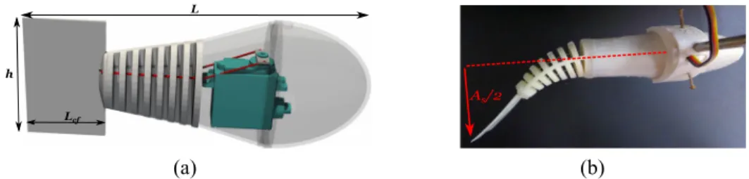
NinjaTek. This elastic material provides the flexibility of the swimmer’s tail, whose shape is shown in Fig.1(a). Two cables were attached to the tail and guided toward the head through the holes of the flexible skeleton. These two cables were glued to a connecting wheel of the waterproof servomotor HS-5086WP from Hitec, which was fixed to both the 3D printed rigid head and flexible skeleton. This choice obviated the problems of sealing the moving parts of the robot. The rotation of the ser-vomotor releases one cable while pulling the other, thereby mimicking the action of two antagonistic muscles. The back and forth rotation of the servomotor wheel causes both an undulation of the flexible tail and a pitching motion. To sim-ulate an outer skin, we quantified the effect of covering the flexible skeleton with a very thin latex sheet and found that it does not affect the measurements within the precision of our devices. Therefore we kept the skeleton uncovered for simplicity.
The robotic fish is held in place by a rod connected to a force sensor [Fig.1(b)], a Honigmann RFS®150E, which
permits measurement of the total longitudinal force with a precision of approximately 10−4N. The positive and negative values of this force are related to a thrust-prevailing regime and drag-prevailing regime, respectively. In addition, the fish is wired to an Arduino Mega micro-controller, which simulta-neously controls the servomotor, acquires data from the force sensor, and drives the fast camera.
We denote U0 as the free stream velocity, F as the time-averaged value of the longitudinal force, L as the total length of the fish, and SD as its projected frontal area at
rest. Further, the fish’s tail consists of a flexible caudal fin with length Lcf and height h [Fig.1(a)]. Unless stated
other-wise (two other caudal fins were also tested, cf. Sec.III A), L = 17 cm, Lcf = 3.6 cm, and h = 6 cm. The caudal fin has
a heterogeneous thickness profile spanning from 1 mm at the contact with the peduncle to 0 mm at its trailing edge. The flow around the fish is characterized by a high Reynolds number, Re = ρU0L/η, with typical values of ∼104.
The head of the fish is fixed by a rod in the reference frame of the lab. The tail of the robotic fish is driven by the deformation of its body through the rotation of the servomotor wheel, whose angular position is denoted as ϕ. Experiments are performed either with a motionless (ϕ is constant) or motile (ϕ(t) depends on time) fish.
For the motionless fish, ϕ = 0◦ corresponds to the fin aligned with the swimmer body. A calibration is then performed without any fluid motion to connect the imposed
FIG. 1. Fish design. (a) 3D representation of the robot. The transparent parts of the robot were printed with a rigid polymer (PLA). The servomotor is drawn in green, and the cables are drawn in red. The soft parts of the robot are opaque and shown in white. The fish has total length L and a tail consisting of a flexible caudal fin with length Lcfand height h. (b) Top view of the compliant fish with an imposed tail deformation (ϕ = 70◦, As= 8.1 cm), the holding rod, and the
091901-3 Gibouin et al. Phys. Fluids 30, 091901 (2018)
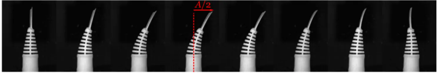
FIG. 2. Image sequence (half of a period) of the swimming fish with the parameters Φ = 100◦, f = 1 Hz, and U0= 0.
angular position ϕ with the deformation of the tail, character-ized by the static amplitude of the fin As[Fig.1(b)].
For the motile fish, the swimming dynamics were studied by imposing a harmonic angular function ϕ(t)= Φ2 sin(2πft), where Φ is the angular amplitude (range 0◦–140◦) and f is the forcing frequency (range 0–1.6 Hz). The tail-beat ampli-tude A, defined as the tip-to-tip excursion of the tail, is directly measured on the image sequence (Fig.2). Because of the inter-action of the tail with water, the tail-beat amplitude A measured with the motile fish at an angular amplitude Φ might be dif-ferent from As measured with the motionless fish at ϕ = Φ/2.
For the motile fish, both the tail-beat amplitude A and average value of the longitudinal force F should be functions of Φ, f, and U0.
Images are recorded with a MINICAM WX50 from Photron. A typical sequence centered on the fish trunk and tail is given in Fig.2. To illustrate the flow in the vicinity of the caudal fin, we implemented a particle image velocimetry (PIV) system along the horizontal medial plane of the fish (see thesupplementary material).
III. RESULTS
We investigate the swimming characteristics of the robotic fish. First, in Sec. III A, we perform experiments in the absence of mean flow (U0 = 0 in the water tunnel) and ana-lyze the amplitude and thrust of the motile fish. Second, in Sec. III B, we exclusively study the drag, i.e., the frictional force exerted on the motionless fish for several static ampli-tudes and free stream velocities. Finally, in Sec.III C, we char-acterize the self-propelled swimming conditions defined as the combinations of parameters A, f, and U0that result in a zero
average longitudinal force, which corresponds to a thrust–drag balance.
A. Thrust analysis
To investigate the thrust alone, we work with a motile fish and remove the drag by taking the free stream velocity U0= 0. Figure3presents the dependence of the amplitude A with respect to the imposed parameters Φ and f. For a given frequency, the higher the Φ, the higher the A. For a given Φ, the amplitude A seems constant for small f. By increas-ing the frequency, the amplitude A increases and reaches a maximum before dropping: this is a characteristic of a res-onant response. We denote fm as the resonant frequency for
which the amplitude is a maximum. This frequency depends on Φ, and we observe that Φ and fm are inversely related
[Fig.3(b)].
This result is consistent with what has been seen before with flexible panels,11,14–16but here, we provide the first results
for a compliant robotic fish. As in Ref.15, this inverse rela-tionship appears to be a consequence of the nonlinear behavior of the system.
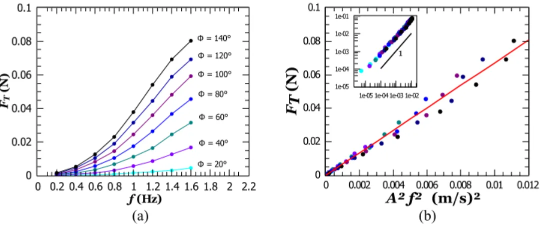
Measurements of the thrust FTfrom the force sensor are
shown in Fig.4(a), where FTis an increasing function of both
Φand f. Plotting FTas a function of A2f2in Fig.4(b)reveals a
linear trend over the whole range of values, down to the preci-sion of the force sensor of approximately 10−4N. This scaling holds over 3 orders of magnitudes for the thrust [as shown in the inset of Fig.4(b)]. Based on Eq.(1), the linear regression leads to CTST= (134 ± 2) × 10−4m2. This result suggests that
our flexible compliant robot exhibits the same A2f2scaling as undulating rigid structures,11,14,35,37irrespective of whether it is resonant or not. This approach conciliates the dynamics of
FIG. 3. (a) A as a function of f for several Φ (20◦, 40◦, 60◦, 80◦, 100◦, 120◦, and 140◦from bottom to top). The red arrow is a guide for the eye to display the
091901-4 Gibouin et al. Phys. Fluids 30, 091901 (2018)
FIG. 4. Thrust measurements. (a) FT
as a function of f for several Φ. (b) FTas
a function of A2f2, with A measured in Fig.3. The solid line is a linear regres-sion, which leads to CTST= (134 ± 2)
×10−4m2in Eq.(1). Inset: log-log plot
of the same data.
flexible structures, whose thrust and amplitude are maximal near the same resonant frequency.16
To validate our observations, we slightly modified the robot so that the caudal fin is interchangeable. Measurements were now performed with three caudal fins (Lcf = 3.6, 6.0,
and 9.2 cm and all with h = 6 cm) with the same experimen-tal protocol. As seen in the image sequences in Fig.5(a), the dynamics of fin deformation for the two longest fins are dif-ferent from the shortest one with Lcf = 3.6 cm. The tip of the
shortest fin is always in phase with the motion of the peduncle, while it can be significantly out of phase for the longest fin. For all three fins, the thrust is still proportional to A2f2, and the proportionality factor is relatively the same [Fig.5(b)]. This is consistent with the results obtained by Quinn et al. on flexible panels performing a heaving motion.14 They found that the thrust does not depend significantly on the panel elasticity or geometry nor on the profile of the panel deformation, as long as the deformation is accounted for by the tail-beat amplitude. These observations seem to hold for our compliant robot as well. In this work, we only considered swimmers with a mod-erate length of the caudal fin, but it would be very engaging to tackle the effects of the deformation modes of long and flexible tails.45–47
B. Drag analysis
To investigate the drag FDalone without any thrust,
mea-surements were performed with a motionless fish and imposing a flow in the water tunnel. The drag values recorded by the force sensor were negative, and we display the absolute values here for simplicity. To quantify geometrical effects, the tail was placed in various off-center positions, which are charac-terized by the static amplitude As[Fig.1(b)]. For each value of
As, the free stream velocity U0 is varied from 0 to 0.105 m/s [Fig.6(a)]. For high Reynolds numbers, FDis proportional to
U2 048and defined by FD= 1 2ρCD(As)SDU 2 0, (2)
where SDis a reference area for the drag and CD(As) is the drag
coefficient. For a measured FDand an imposed As, CD(As)SD
is computed using Eq.(2). For the centered tail, the measure-ments lead to CD(0)SD= (25.2 ± 0.3) × 10−4m2. By using the
wetting area as a reference for SD(approximated to 135 cm2),
we estimate CD(0) = 0.19. We then plot CD(As)/CD(0) as a
function of As in Fig. 6(b) and observe a parabolic trend.
An off-centered tail augments the projected frontal area of the fish, resulting in a drag magnification when As becomes
large enough. But this relative increase in the projected frontal area, which is proportional to As, is not enough to explain the
quadratic behavior of the drag coefficient seen in Fig. 6(b). An analogy can be made with airfoils, whose drag coeffi-cient is a quadratic function of the incidence angle.49 The trend observed in Fig.6(b)is captured by the simple parabola 1 + (As/A0)2, where A0is the length. Although this correction might be understood as ad hoc, we rationalize this quadratic behavior by considering the symmetry As→ −Asin the
Tay-lor expansion of the drag coefficient within the small Aslimit.
This development permits to account for both the effect of the projected frontal area and of the geometry in the determination of CD(As).
The best fit gives A0 = 0.089 ± 0.002 m. Therefore, we can infer the following expression for the drag force:
FD=
1
2ρCD(0)SDU 2
0[1 + (As/A0)2]. (3)
FIG. 5. Effect of the caudal fin design on the thrust. (a) Image sequence over one period for each fin with the param-eters Φ = 60◦, f = 1.2 Hz, and U
0= 0.
091901-5 Gibouin et al. Phys. Fluids 30, 091901 (2018)
FIG. 6. Drag force measurements. (a)
FD as a function of U02 for several
static fin positions (As varies between
0 and 0.081 m). Solid lines are linear fits for the two extreme values of As.
Inset: log-log plot of the same data. (b) CD(As)/CD(0) as a function of As.
A parabolic fit CD(As)/CD(0) = 1 +
(As/A0)2leads to A0= 0.089 ± 0.002
m.
The drag exerted on a static fish exhibits nonlinear behav-ior connected to the amplitude As of the caudal fin. The
length A0characterizes this effect, and it is not surprising that its value has the same order of magnitude as the length of the fish. The drag expression for a motionless fish will be useful to compare with the dynamic case of a motile fish below.
C. Self-propelled swimming conditions
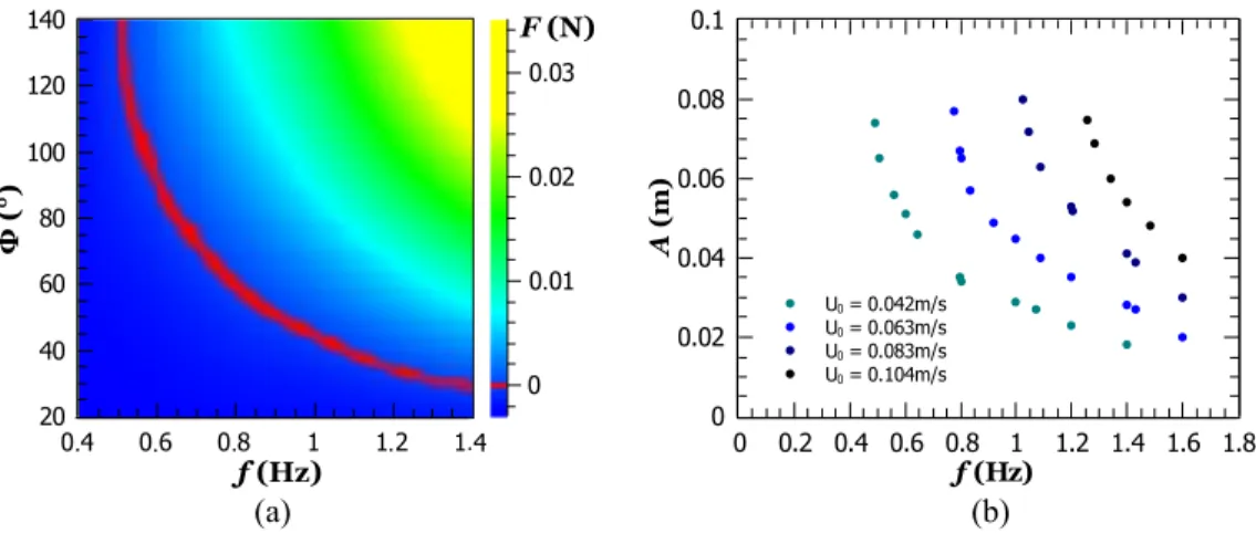
Experiments are now carried out with a motile fish and an imposed flow in the water tunnel. The average force F and the tail-beat amplitude A are functions of Φ, f, and U0. For a given velocity U0, the force is represented as a 2D map displaying both the thrust-prevailing (positive values) and the drag-prevailing (negative values) zones [Fig.7(a)].
At the frontier of these two regions, the thrust and drag counterbalance each other (F = 0), and the fish is self-propelled. Each set of parameters (A, f, U0) fulfilling F = 0 defines a self-propelled condition. All of them are represented in Fig.7(b): for a given U0, larger f results in smaller A, while increasing U0 shifts the points of self-propulsion toward the larger values of A and f.
To account for these measurements, we use the expres-sions of the thrust and drag obtained independently [Eqs.(1)
and(3)] and assume that both expressions still hold for the self-propelled swimming conditions. For the drag expression, we replace A by As. The balance FT = FDleads to
Af U0 = St = St0 s 1 + A A0 !2 , (4) with St0= q CD(0)SD
CTST as the Strouhal number at a small
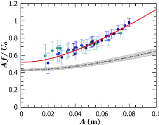
ampli-tude (A A0). This expression is tested with the self-propelled data by plotting the Strouhal number St = Af /U0as a function of A (Fig.8). All data collapse on the same curve regardless of the free stream velocity or tail-beat frequency. Consistent with Eq.(4), the Strouhal number is an increasing function of the tail-beat amplitude only.
A quantitative comparison with the model obtained from the independent thrust and drag analyses (St0= 0.43 ± 0.01 and A0= 0.089 ± 0.002 m, black dashed line in Fig.8) shows that the self-propelled data systematically lead to higher values of the Strouhal number. Actually a two-parameter interpolation with these data instead yields St0= 0.52 ± 0.05 and A0= 0.052 ±0.005 m (red solid line in Fig.8). There is a 19% difference between the values of St0. Given the lack of data for A < 0.02 m and in the limit A A0and since the error bars of the data points are greater for smaller A, it is not clear whether or not this difference is significant nor whether the extrapolation toward A = 0 would lead to a smaller difference or not. In this con-text, we prefer to say that our model without free parameters validates the independent thrust and drag analyses at small amplitudes within a margin of 19%.
Unlike the small amplitude regime (A A0), the interme-diate amplitude regime (A ∼ A0) is characterized by numerous
FIG. 7. (a) Time-averaged force F as a function of Φ and f for a given free stream velocity U0= 0.042 m s−1. The red line corresponds to the pairs of (Φ, f )
091901-6 Gibouin et al. Phys. Fluids 30, 091901 (2018)
FIG. 8. Strouhal number St = Af /U0 as a function of A for the data of
Fig.7(b). The red solid line is a two-parameter interpolation with the full model, St0
q
1 + (A/A0)2, and the black dashed line with the gray error bars is
the model with the parameters inferred from the independent thrust and drag analyses.
data points, and all of them have significantly larger values than the prediction based on the independent thrust–drag anal-yses. For the largest values, the difference reaches almost 50%. This means that the approach does not hold any more and that the motile fish gives rise to a larger effective drag than expected from the independent thrust–drag analyses. Actually the difference between the static drag and the real drag expe-rienced by the motile fish is characterized by almost a factor two between the two predictions of A0. This difference might be partly understood by considering the effective frontal area as one possible contribution: for instance, in the limit of high frequencies, one could model the swimmer as a solid object, whose increase in effective frontal area with the fin amplitude is doubled compared to the static case as the fin is flapping on both sides of the fish.
IV. DISCUSSION AND CONCLUSIONS
Our analysis shows that the Strouhal number of a self-propelled flexible swimmer is not necessarily constant but an increasing function of the tail-beat amplitude. At small ampli-tudes, the model based on the independent analyses of thrust and drag is rather good, given that there is no free parameter. These results provide evidence that the Strouhal number of a self-propelled swimmer is associated with the thrust–drag balance22,27and that performing independent analyses is rel-evant to characterize the swimming properties to the leading order.
For biological swimmers, the Strouhal number appears to be a constant over a large number of decades of the Reynolds number,22 as well as the second dimensionless number,
A/L ∼ 0.2.26–29This constancy might be rationalized with a
principle of minimum energy consumption.27Unfortunately
it was not possible to measure the energy consumption of our system. Nevertheless, our experimental setup has permit-ted to explore the effect of A/L, and we demonstrate that the Strouhal number is amended by a correction factor induced by the amplitude on the effective drag.
The values of our Strouhal number at small amplitudes are found around 0.5 in comparison with natural swimmers (average on the order of 0.322,27). This result suggests that
the thrust coefficient is smaller and/or the drag coefficient is larger than those of an average natural swimmer. The fact that the motion of the robot is a pure pitch could explain this obser-vation. Adding a degree of heaving in the design of the robot might decrease the values of the Strouhal number.
SUPPLEMENTARY MATERIAL
Seesupplementary materialfor movies illustrating the tail oscillation of the motile fish (3 caudal fins, Lcf = 3.6, 6.0, and
9.2 cm, with the parameters Φ = 60◦, f = 1.2 Hz, and U0= 0) and the flow in the vicinity of the caudal fin by particle image velocimetry.
ACKNOWLEDGMENTS
We thank R. Todres for the thorough reading of the manuscript. We are grateful to P. Vignolo for his valuable assistance in seeking funding sources. F. Gibouin thanks the financial support of the CNRS. The authors acknowl-edge project funding by the UCAJEDI IDEX Grant (No. ANR-15-IDEX-01).
1T. Theodorsen, “General theory of aerodynamic instability and the
mech-anism of flutter,” Report No. 496, National Advisory Committee for Aeronautics, Washington, D.C., 1935.
2I. E. Garrick, “Propulsion of a flapping and oscillating airfoil,” Report
No. 567, National Advisory Committee for Aeronautics, Washington, D.C., 1936.
3M. Koochesfahani, “Vortical patterns in the wake of an oscillating airfoil,”
in 25th AIAA Aerospace Sciences Meeting (AIAA, 1987).
4G. Triantafyllou, M. Triantafyllou, and M. Grosenbaugh, “Optimal thrust
development in oscillating foils with application to fish propulsion,” J. Fluids Struct.7(2), 205–224 (1993).
5L. Schouveiler, F. Hover, and M. Triantafyllou, “Performance of flapping
foil propulsion,”J. Fluids Struct.20(7), 949–959 (2005).
6J. Anderson, K. Streitlien, D. Barrett, and M. Triantafyllou, “Oscillating
foils of high propulsive efficiency,”J. Fluid Mech.360, 41–72 (1998).
7D. A. Read, F. Hover, and M. Triantafyllou, “Forces on oscillating
foils for propulsion and maneuvering,”J. Fluids Struct.17(1), 163–183 (2003).
8M. J. Lighthill, “Note on the swimming of slender fish,”J. Fluid Mech.9(2),
305–317 (1960).
9M. J. Lighthill, “Aquatic animal propulsion of high hydromechanical
efficiency,”J. Fluid Mech.44(2), 265–301 (1970).
10K. Moored, P. Dewey, A. Smits, and H. Haj-Hariri, “Hydrodynamic wake
resonance as an underlying principle of efficient unsteady propulsion,”J. Fluid Mech.708, 329–348 (2012).
11P. A. Dewey, B. M. Boschitsch, K. W. Moored, H. A. Stone, and A. J. Smits,
“Scaling laws for the thrust production of flexible pitching panels,”J. Fluid Mech.732, 29–46 (2013).
12C. Marais, B. Thiria, J. E. Wesfreid, and R. Godoy-Diana, “Stabilizing effect
of flexibility in the wake of a flapping foil,”J. Fluid Mech.710, 659–669 (2012).
13S. Alben, C. Witt, T. V. Baker, E. Anderson, and G. V. Lauder, “Dynamics
of freely swimming flexible foils,”Phys. Fluids24(5), 051901 (2012).
14D. B. Quinn, G. V. Lauder, and A. J. Smits, “Scaling the propulsive
performance of heaving flexible panels,”J. Fluid Mech.738, 250–267 (2014).
15F. Paraz, C. Eloy, and L. Schouveiler, “Experimental study of the response
of a flexible plate to a harmonic forcing in a flow,”C. R. Mec.342(9), 532–538 (2014).
16F. Paraz, L. Schouveiler, and C. Eloy, “Thrust generation by a heaving
flexible foil: Resonance, nonlinearities, and optimality,”Phys. Fluids28(1), 011903 (2016).
17C. J. Esposito, J. L. Tangorra, B. E. Flammang, and G. V. Lauder, “A
robotic fish caudal fin: Effects of stiffness and motor program on locomotor performance,”J. Exp. Biol.215(1), 56–67 (2012).
091901-7 Gibouin et al. Phys. Fluids 30, 091901 (2018)
18A. J. Richards and P. Oshkai, “Effect of the stiffness, inertia and
oscilla-tion kinematics on the thrust generaoscilla-tion and efficiency of an oscillating-foil propulsion system,”J. Fluids Struct.57, 357–374 (2015).
19S. G. Park, B. Kim, and H. J. Sung, “Hydrodynamics of a self-propelled
flexible fin near the ground,”Phys. Fluids29(5), 051902 (2017).
20S. Ramananarivo, R. Godoy-Diana, and B. Thiria, “Rather than resonance,
flapping wing flyers may play on aerodynamics to improve performance,”
Proc. Natl. Acad. Sci. U. S. A.108(15), 5964–5969 (2011).
21M. Gazzola, M. Argentina, and L. Mahadevan, “Gait and speed selection
in slender inertial swimmers,”Proc. Natl. Acad. Sci. U. S. A.112(13), 3874–3879 (2015).
22M. Gazzola, M. Argentina, and L. Mahadevan, “Scaling macroscopic
aquatic locomotion,”Nat. Phys.10(10), 758 (2014).
23M. S. Triantafyllou, G. S. Triantafyllou, and R. Gopalkrishnan, “Wake
mechanics for thrust generation in oscillating foils,”Phys. Fluids A3, 2835–2837 (1991).
24M. S. Triantafyllou, G. Triantafyllou, and D. Yue, “Hydrodynamics of
fishlike swimming,”Annu. Rev. Fluid. Mech.32(1), 33–53 (2000).
25G. K. Taylor, R. L. Nudds, and A. L. Thomas, “Flying and swimming
animals cruise at a Strouhal number tuned for high power efficiency,”Nature
425(6959), 707–711 (2003).
26J. J. Rohr and F. E. Fish, “Strouhal numbers and optimization of swimming
by odontocete cetaceans,”J. Exp. Biol.207, 1633–1642 (2004).
27M. Saadat, F. Fish, A. Domel, V. Di Santo, G. Lauder, and H. Haj-Hariri, “On
the rules for aquatic locomotion,”Phys. Rev. Fluids2(8), 083102 (2017).
28R. Bainbridge, “The speed of swimming of fish as related to size and to
the frequency and amplitude of the tail beat,” J. Exp. Biol. 35(1), 109–133 (1958).
29J. R. Hunter and J. R. Zweifel, “Swimming speed, tail beat frequency, tail
beat amplitude, and size in Jack mackerel, Trachurus symmetricus, and other fishes,” Fish. Bull. 69(2), 253–266 (1971).
30M. G. Chopra and T. Kambe, “Hydromechanics of lunate-tail swimming
propulsion. Part 2,”J. Fluid Mech.79(1), 49–69 (1977).
31G. Karpouzian, G. Spedding, and H. K. Cheng, “Lunate-tail swimming
propulsion. Part 2. Performance analysis,”J. Fluid Mech.210, 329–351 (1990).
32H. Dong, R. Mittal, and F. M. Najjar, “Wake topology and hydrodynamic
performance of low-aspect-ratio flapping foils,”J. Fluid Mech.566, 309– 343 (2006).
33J. H. J. Buchholz and A. J. Smits, “The wake structure and thrust
per-formance of a rigid low-aspect-ratio pitching panel,”J. Fluid Mech.603, 331–365 (2008).
34M. A. Green and A. J. Smits, “Effects of three-dimensionality on thrust
production by a pitching panel,”J. Fluid Mech.615, 211–220 (2008).
35T. Van Buren, D. Floryan, N. Wei, and A. J. Smits, “Flow speed has little
impact on propulsive characteristics of oscillating foils,”Phys. Rev. Fluids
3, 013103 (2018).
36M. J. Lighthill, “Hydromechanics of aquatic animal propulsion,”Annu. Rev.
Fluid Mech.1(1), 413–446 (1969).
37D. Floryan, T. Van Buren, C. W. Rowley, and A. J. Smits, “Scaling the
propulsive performance of heaving and pitching foils,”J. Fluid Mech.822, 386–397 (2017).
38M. S. Triantafyllou and G. S. Triantafyllou, “An efficient swimming
machine,”Sci. Am.272(3), 64–70 (1995).
39H. Hu, “Biologically inspired design of autonomous robotic fish at essex,”
in Proceedings of the IEEE SMC UK-RI Chapter Conference (IEEE, 2006), pp. 1–8.
40P. P. A. Valdivia y Alvarado, “Design of biomimetic compliant devices for
locomotion in liquid environments,” Ph.D. thesis, Massachusetts Institute of Technology, 2007.
41F. Boyer, D. Chablat, P. Lemoine, and P. Wenger, “The eel-like robot,”
inProceedings of ASME Design Engineering Technical Conference and Computers and Information in Engineering Conference, San Diego, CA (ASME, 2009), pp. 655–662, DETC2009-86328.
42C. Stefanini, S. Orofino, L. Manfredi, S. Mintchev, S. Marrazza, T. Assaf,
L. Capantini, E. Sinibaldi, S. Grillner, P. Wallen et al., “A compliant bioin-spired swimming robot with neuro-inbioin-spired control and autonomous behav-ior,” in 2012 IEEE International Conference on Robotics and Automation
(ICRA) (IEEE, 2012), pp. 5094–5098.
43H. El Daou, T. Salum¨ae, G. Toming, and M. Kruusmaa, “A bio-inspired
compliant robotic fish: Design and experiments,” in 2012 IEEE
Inter-national Conference on Robotics and Automation (ICRA) (IEEE, 2012),
pp. 5340–5345.
44Y. Cha, J. Laut, P. Phamduy, and M. Porfiri, “Swimming robots have
scaling laws, too,” IEEE/ASME Trans. Mechatronics 21(1), 598–600 (2016).
45M. Pi˜neirua, B. Thiria, and R. Godoy-Diana, “Modelling of an actuated
elastic swimmer,”J. Fluid Mech.829, 731–750 (2017).
46A. Crespi, K. Karakasiliotis, A. Guignard, and A. J. Ijspeert, “Salamandra
robotica II: An amphibious robot to study salamander-like swimming and walking gaits,”IEEE Trans. Rob.29(2), 308–320 (2013).
47T. Leclercq and E. de Langre, “Reconfiguration of elastic blades in
oscillatory flow,”J. Fluid Mech.838, 606–630 (2018).
48G. K. Batchelor, An Introduction to Fluid Dynamics (Cambridge University
Press, 2000).
49F. D. Bianchi, H. de Battista, and R. J. Mantz, Wind Turbine Control Sys-tems: Principles, Modelling and Gain Scheduling Design (Springer-Verlag,