HAL Id: hal-01054669
https://hal.archives-ouvertes.fr/hal-01054669
Submitted on 8 Aug 2014
HAL is a multi-disciplinary open access
archive for the deposit and dissemination of
sci-entific research documents, whether they are
pub-lished or not. The documents may come from
teaching and research institutions in France or
abroad, or from public or private research centers.
L’archive ouverte pluridisciplinaire HAL, est
destinée au dépôt et à la diffusion de documents
scientifiques de niveau recherche, publiés ou non,
émanant des établissements d’enseignement et de
recherche français ou étrangers, des laboratoires
publics ou privés.
Marangoni induced force on a drop in a Hele Shaw cell
Francois Gallaire, Philippe Meliga, Patrice Laure, Charles N. Baroud
To cite this version:
Francois Gallaire, Philippe Meliga, Patrice Laure, Charles N. Baroud. Marangoni induced force on a
drop in a Hele Shaw cell. Physics of Fluids, American Institute of Physics, 2014, 26 (6), pp.062105.
�10.1063/1.4878095�. �hal-01054669�
Marangoni induced force on a drop in a Hele Shaw cell
Franc¸ois Gallaire,1Philippe Meliga,2Patrice Laure,3and Charles N. Baroud4
1LFMI, EPFL, Lausanne, Switzerland
2M2P2, CNRS and Aix-Marseille University, Marseille, France
3Laboratoire J. A. Dieudonn´e Universit´e de Nice-Sophia Antipolis, Parc Valrose,
F-06108 Nice Cedex 02, France
4LadHyX and Department of Mechanics, Ecole Polytechnique, 91128 Palaiseau, France (Received 18 February 2014; accepted 20 March 2014; published online 13 June 2014)
We analyse the force balance on a cylindrical drop in a Hele-Shaw cell, subjected to a Marangoni flow caused by a surface tension gradient. Depth-averaged Stokes equa-tions, called Brinkman equaequa-tions, are introduced and a general closed form solution is obtained. The validity of the averaging procedure is ascertained by considering a linear surface tension gradient acting on a cylindrical flattened drop. The Marangoni-driven flow field and resulting force predicted by the Brinkman model are seen to match well a full three-dimensional direct numerical simulation. A closed form ex-pression of the force acting on the drop is obtained, calculated from contributions due to the normal viscous stress, tangential viscous stress, and pressure fields, integrated on the drop perimeter. This expression is used to predict the force balance when a sta-tionary droplet is submitted to both a carrier flow and a Marangoni flow. We show that previous results in the literature had underestimated by a factor two the Marangoni-induced force.!C 2014 AIP Publishing LLC. [http://dx.doi.org/10.1063/1.4878095]
I. INTRODUCTION
Droplet-based microfluidics has developed into a highly active area in recent years, owing to its ability to answer some major issues facing single phase flows. In particular, the use of droplets reduces the problem of handling small volumes to the manipulation of a single droplet, which provides an elegant approach to performing reactions with minute volumes since the contents of a drop can remain within the drop if the liquids are chosen properly. In addition, the recirculation motion inside the drop induced by the shear imposed on the immiscible interface through the surrounding carrier flow can be used to mix the drop contents.
This has renewed interest in Marangoni effects acting on drops, with the active modulation of surface stresses being proposed as a manipulation tool for droplets either inside or outside microchannels.1 Lasers were used to locally heat a water-oil interface in the confined geometry of microchannels and this technique was used to implement all of the necessary operations on droplets.2–4In this approach, the heating produced by the focused laser leads to a thermocapillary stress that is generated on the drop surface. Owing to the low Reynolds numbers, this almost instan-taneously produces a flow in the inner and outer fluids, while the drop translation is simulinstan-taneously blocked as its interface reaches the laser spot. These experiments therefore demonstrate the produc-tion of a net force that can balance the viscous drag on a locally heated droplet, generating forces of a few hundred nano Newtons.5The direction of the force was found to be pointing away from the hot spot, similar to the direction observed by Kotz et al.6and Grigoriev et al.7in spherical geometry, but in disagreement with classical results which predict that drops should migrate towards the hot regions (e.g., Young, Goldstein, and Block8). This was attributed by Verneuil et al.5to the direction of the Marangoni rolls, due to the presence of partially soluble surfactants that were depleted by the laser, while Selva et al.,9 showed that the force oriented towards the cold side was driven in their experimental setup by the cell deformation in response to thermal stresses.
While these authors confirmed experimentally the Marangoni origin of the force, several ques-tions remain about the hydrodynamics and the scalings behaviour of such forcing methods. This leads us to revisit the problem of the force acting on a drop in a Hele-Shaw geometry, treated in the literature by the work of Nadim et al.,10Boos and Thess,11and Bush.12These three studies addressed the effect of Marangoni stresses, due to a temperature or surfactant concentration gradient, on the motion of a flattened drop or bubble. Nadim et al.10calculated the tangential stress effects caused by a linear surface temperature distribution on a flat fluid-fluid interface and used this result to derive the velocity of a circular bubble in a constant temperature gradient. We will show that these prediction underestimate the real force by a factor two. Boos and Thess11 determined the flow in detail using depth-averaged (so-called Brinkman) equations and conducted numerical computations of the velocity field for complex shaped bubbles, using a simplifying boundary layer approximation. Finally, Bush12derived an expression for the terminal velocity of a buoyancy driven flattened bubble and showed that it could be retarded by a secondary solutal Marangoni flow.
The aim of the present study is to calculate the forces acting on a stationary drop or bubble in a Hele-Shaw cell in the presence of a surface tension gradient and of an external flow, in the spirit of Hadamard,13 Rybzynski,14 and Young et al.8 This first leads us to generalize Boos and Thess’s11 solution of the Brinkman equations for an arbitrary general surface tension distribution. The stress distribution predicted by the depth-averaged procedure inherent to the Brinkman model is then quantitatively validated by comparison with three-dimensional (3D) numerical computations of the Stokes equations, enabling us to obtain a generic closed form expression of the force acting on a stationary droplet. The equilibrium conditions under which the force exerted by the carrier fluid is exactly cancelled by the Marangoni effect are finally determined.
The governing equations for the inner and outer flows around a flattened drop are posed in Sec. IIand a numerical solution procedure is proposed in Sec. III. The depth-averaged, so-called Brinkman equations are introduced and solved in Sec.IVin the cases of local or global variations of surface tension. In Sec. V, the validity of the approach is assessed by comparing the stress fields predicted theoretically in the frame of the Brinkman approximation with those obtained from three-dimensional Stokes simulations. This enables determining the generic force expression on a stationary droplet for any arbitrary flow and allows computing the force caused either by a Marangoni flow on a stationary drop (Sec.VI) or by an incoming flow on a stationary droplet (Sec.VII). The tentative application of our approach to translating droplets follows in Sec.VIIIbefore conclusions and perspectives are drawn in Sec.IX.
II. PROBLEM STATEMENT
Let us consider a cylindrical flattened drop or bubble of radius ¯Rand viscosity ¯µ1, surrounded by a stationary or constantly flowing (at velocity ¯U∞) fluid of viscosity ¯µ2, in a Hele-Shaw cell of gap ¯h small compared to ¯R, as depicted in Figure1(dimensional variables are denoted with an overbar). The two fluids are immiscible and subject to a surface tension ¯γ =γ¯0+"γ γ¯ which may vary in space with an amplitude " ¯γ. This surface tension distribution is assumed to remain frozen. It may result either from a temperature ¯T = ¯T0+" ¯T T or surfactant concentration ¯c = ¯c0+"¯c c distribution, the resulting surface tension variation " ¯γ = ¯GT" ¯T or " ¯γ = ¯Gc"¯c being obtained
er eθ θ h y x z R
using a scalar coefficient ¯Gcor ¯GT. We shall assume the Reynolds number Re = ¯U ¯R/( ¯µ1+µ¯2) based on the radius of the drop ¯R, the total viscosity ¯µ1+µ¯2, and the characteristic velocity ¯U to be small. Depending on the flow configuration, this reference velocity ¯U is either the characteristic Marangoni velocity ¯Um="γ ¯¯h/ ¯R( ¯µ1+µ¯2) or the external carrier fluid velocity ¯U∞. In order to non-dimensionalize the equations, we therefore use the radius of the drop ¯R as characteristic length-scale, the reference time and force scale being ( ¯µ1+µ¯2) ¯R
"γ¯ and " ¯γ ¯R(respectively, ¯R/ ¯U∞and ¯
R( ¯µ1+µ¯2) ¯U∞) when the droplet is submitted to Marangoni forcing (respectively, when submitted to a uniform carrier flow). Nondimensional quantities are denoted without overbar.
With the assumption of a low Reynolds number, the equations of motion reduce to the 3D Stokes equations,
µi"V(i )= ∇ Pi, (1)
∇.V(i )=0, (2)
where the pressure is denoted by Piand where the index i = 1, 2 refers to fluids 1 and 2.
With the exception of Sec.VIII(where the results are extended tentatively to moving droplets), the present study focuses on stationary droplets. In this situation, the droplets adopt toroidal-like shapes with the geometric details of the rim depending on the wetting properties. For droplet wetting the channel walls, the droplet is directly in contact with the solid walls and the rim geometry is set by the contact angle. For non-wetting droplets, a thin molecular film is caused by the disjunction pressure and the rim has a shape that becomes asymptotically close to a semi-circle of radius of curvature equal to the half-height of the channel h/2 as h/R tends to 0. The existence of this curved rim is neglected in the present study, following Boos and Thess11and Bush.12The droplet interface thereby reduces to a flattened cylinder which we further assume to be circular, assuming that the capillary number is sufficiently low for the droplet not to depart from its equilibrium shape in absence of flow. Although this assumption of a prescribed shape of the interface precludes the imposition of the normal stress boundary condition, it is a reasonable assumption as long as the capillary number is small enough.
In addition, observe that this classical assumption in low-Reynolds number two-phase flows8,13,14 can in certain cases be validated a posteriori. Such a “unique result”15 happens for the low Reynolds translational motion of a spherical droplet or its motion under a linear surface tension gradient, where it was checked8,13,14 that the spherical shape does indeed ensure the local normal stress balance along the interface. It can be shown however, that in the present case of a pancake droplet flowing in a Hele-Shaw cell, the circular shape does not ensure the local normal stress balance.
The remaining boundary conditions consist of impermeability and continuity of both tangential velocities and tangential shear stresses, where tk(k = 1, 2) denote the two unit tangent vectors and T(i)the stress tensors
V(i )!!z=±1/2= 0, (3) V(i ).n!!r =1 =0, (4) V(1).tk ! !r =1 = V(2).tk ! !r =1, (5) tk.T(1).n!!r =1 = tk.T(2).n ! !r =1+ ∇γ.tk. (6)
III. A REFERENCE NUMERICAL SOLUTION
With the aim to validate in Sec.Vthe depth-averaged model used in the remainder of the study, let us first obtain in this section a reference direct numerical simulation of the 3D Stokes equations.
We consider the effect of an imposed surface tension profile, generated, for example, by an imposed temperature field. We assume for the sake of clarity that the surface tension along the interface γ (θ ) is an even function (we anticipate in this way the null contribution of the odd part of the function to the net x-directed force). Its gradient may then be decomposed onto the sine modes only (calculations can be extended to cosine modes contributions in a straightforward manner)
dγ dθ = ∞ " n=1 ansin(nθ ), (7) where an = 1 π # 2π 0 dγ dθ sin(nθ )dθ. (8)
In this section, we solve numerically the 3D Stokes equations(2)–(6)in the case of a linear surface tension gradient acting on a cylindrical interface (γ (r, z, θ ) = cos (θ )). We take advantage of the following (so-called n = 1) azimuthal dependences:
Vr(i )(r, z, θ ) = vr(i )(r, z) cos(θ ), (9)
Vθ(i )(r, z, θ ) = v(i )θ (r, z) sin(θ ), (10) Vz(i )(r, z, θ ) = v(i )z (r, z) cos(θ ), (11) P(i )(r, z, θ ) = q(i )(r, z) cos(θ ) + P0(i ), (12) to transform the 3D stokes equations exactly into the 3C-2D (three components and two dimensions) n =1-Stokes equations given as
∂ ∂r $ 1 r ∂r v(i ) r ∂r % −v (i ) r r2 − 2vθ(i ) r2 + ∂2v(i ) r ∂z2 = ∂q(i ) ∂r , (13) ∂ ∂r & 1 r ∂r vθ(i ) ∂r ' −v (i ) θ r2 − 2v(i )r r2 + ∂2vθ(i ) ∂z2 = − q(i ) r , (14) 1 r ∂ ∂r $ r∂v (i ) z ∂r % −v (i ) z r2 + ∂2v(i ) z ∂z2 = ∂q(i ) ∂z , (15) 1 r ∂ ∂r (rv (i ) r ) + vθ(i ) r + ∂v(i )z ∂z =0, (16)
with suitable boundary conditions derived from Eqs.(3)–(6). Observe that the pressure references P0(i ) in the two fluids are arbitrary since the normal dynamic boundary condition is not imposed. Similar decompositions can be applied to the different elements of the viscous stress tensors, for instance, the tangential stress component Tr θ(i )(r, z, θ ) = t
(i )
r θ(r, z) sin(θ ).
We use the FreeFem++ software (http://www.freefem.org) to generate a two-dimensional triangulation of the azimuthal plane with the Delaunay–Voronoi algorithm. The mesh refinement is controlled by the vertex densities imposed on both external and internal boundaries. All equations are numerically solved by a finite-element method using two meshes, one for the interior domain and one for the exterior domain. Each set of equations is first multiplied by r to avoid the singularity on the r =0 axis. The associated variational formulation is then derived and spatially discretized onto a basis of Arnold-Brezzi-Fortin MINI-elements,16,17with 4-node P1belements for the velocity components and 3-node P1elements for the pressure. The sparse matrices resulting from the projection of these variational formulations onto the basis of finite elements are built with the FreeFem++ software. The reference results presented in the following have been obtained for interior and exterior meshes, respectively, made of 91 656 triangles and 520 204 triangles, and have been checked to be converged with respect to mesh-refinement.
-0.5 -0.25 0 0.25 0.5 -0.045 -0.03 -0.015 0 -0.4 0.4 z x y R -0.04 0.04 (a) (b)
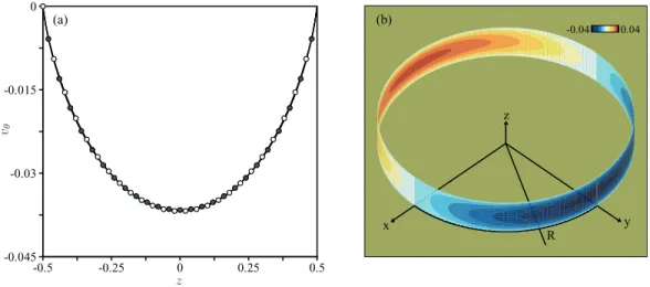
FIG. 2. (a) Transverse tangential velocity profile v(i )θ (1, z); empty (resp. full) symbols correspond to the inner (resp. outer) fluid i = 1 (resp. i = 2). (b) Reconstruction of the tangential velocity field Vθ(i )(1, z, θ ) on the inner and outer surfaces of the drop, as obtained by solving the exact 3C-2D n = 1 Stokes equations; h = 0.1, a1=1, µ1=3/4, and µ2=1/4.
Our approach consists of solving back and forth the n = 1-Stokes equations in each domain. Starting from a guess solution, we solve first the equations in the interior domain 1 with the stress along the interface being imposed by the outer fluid. Then, we solve back the equations in the exterior domain 2 with the stress being now imposed by the inner fluid. We repeat the computations until the following criterion $v1− v2$I nt er f ace<10−3 is satisfied, thereby assuring continuity of the tangential and axial velocities. This simple, segregated scheme was found to converge rapidly (within 5 iterations) for the linear set of equations at hand.
Simulations were run for different parameters, and always showed that the out of plane z component of the velocity v(i )
z was at least one order of magnitude smaller than the in-plane components of the velocity. Figure2(a)depicts the interfacial tangential velocity profiles vθ(1)(1, z) = v(2)θ (1, z), obtained for h = 0.1, a1 =1, µ1 = 3/4, and µ2 =1/4. They display a characteristic parabolic-like profile. In addition, a two-dimensional reconstruction of the surface inner and outer velocities is shown in Figure2(b).
The Marangoni stress discontinuity (here nondimensionalized to 1) is recovered by subtracting the outer shear from the inner one, as seen in Figure3(a), which depicts the interfacial tangential shear stress profiles tr,θ(1)(1, z) and t
(2)
r,θ(1, z), except in the extreme vicinity of the walls. The associ-ated two-dimensional reconstructions of the surface inner and outer shear stresses are depicted in Figure3(b).
The interfacial pressures depicted in Figure4highlight the invariance of the 3D pressure field with respect to z. For completeness, the normal viscous stress components on the interface are also reported in Figure5where they are seen to be one order of magnitude less than the pressure stresses.
IV. DEPTH-AVERAGED MODELLING
Classically, the smallness of the aspect ratio h = ¯h/ ¯R is exploited to separate the wall nor-mal dependance (i.e., in the direction z) of all the velocity fields from its in-plane averaged value
V(i )(x, y, z) = u(i )(x, y)$ 6z(h − z)
h2 %
-0.5 -0.25 0 0.25 0.5 -0.8 -0.4 0 0.4 -0.7 0.7 z x y R -0.7 0.7 (a) (b)
FIG. 3. (a) Transverse tangential stress profile tr,θ(1)(1, z) (empty symbols for the inner fluid) and tr,θ(2)(1, z) (full symbols for the outer fluid); (b) Reconstruction of the tangential stress fields Tr,θ(i )(1, θ, z) on the “inner” and “outer” surfaces of the drop;
h =0.1, a1=1, µ1=3/4, and µ2=1/4.
At leading order, the pressure does not depend on z and the z-component of the velocity may be neglected, yielding the depth-averaged equations
µi("$− 12/ h2) u(i )= ∇$pi, (18) ∇$.u(i )=0, (19) where "$=*∂∂x22 + ∂2 ∂y2 +
is the in-plane Laplacian and ∇$ = * ∂ ∂x, ∂ ∂y +
the in-plane gradient. Equa-tions(18)and(19)are called Brinkman equations;12they combine the classical Darcy approximation of Hele-Shaw flows with the next order O*hR¯¯22
+
Stokes correction. Despite its lower order, it is ju-dicious, although mathematically disputable,18 to include this term in order to satisfy Marangoni boundary conditions. -0.5 -0.25 0 0.25 0.5 0 0.3 0.6 0.9 -0.7 0.7 z x y R -0.8 0.8 (a) (b)
FIG. 4. (a) Transverse pressure profile q(1)(1, z) and q(2)(1, z). (b) Reconstruction of the pressure fields P(i)(1, z, θ ) on the inner and outer surfaces of the drop; h = 0.1, a1=1, µ1=3/4, and µ2=1/4.
z -0.5 -0.25 0 0.25 0.5 0 0.02 0.04 0.06 -0.05 z x y R -0.05 0.05 (a) (b)
FIG. 5. (a) Transverse normal viscous stress profile tr,r(1)(1, z) and tr,r(2)(1, z); (b) Reconstruction of the normal viscous stress field Trr(i )(1, z, θ ) on the inner and outer surfaces of the drop; h = 0.1, a1=1, µ1=3/4, and µ2=1/4.
It is natural at this stage to introduce depth-averaged in-plane streamfunctions ψ(i)such that u(i )θ = −∂ψ (i ) ∂r , (20) u(i )r = 1 r ∂ψ(i ) ∂θ , (21)
which allow rephrasing(18)in cylindrical coordinates (see Boos and Thess11for details) as $ 1 r ∂ ∂rr ∂ ∂r + 1 r2 ∂2 ∂θ2 % $ 1 r ∂ ∂rr ∂ ∂r + 1 r2 ∂2 ∂θ2 − k 2 % ψ(i )=0, (22)
where we have introduced the aspect ratio k =√12 ¯R/ ¯h, assumed to be large. The above equations are valid in each fluid and are closed by suitable boundary conditions on the interface. The kinematic boundary conditions at r = 1 impose equal normal velocities along the interface
ψ(1)!!r =1=ψ(2) !
!r =1, (23)
as well as the continuity of the tangential velocity ∂ψ(1) ∂r ! ! ! !r =1 = ∂ψ (2) ∂r ! ! ! !r =1 . (24)
Except in Sec.VIII, the droplet is considered at rest, which further allows to specify(23)to ψ(1)!!r =1= ψ(2)
!
!r =1=0. (25)
The tangential dynamic boundary condition, which accounts for the Marangoni effect, writes τ1,θ(1) = τ1,θ(2)+ 1rdγdθ
! !
!r =1, where τ is the depth-averaged viscous stress tensor, and can be re-expressed as
µ1r ∂ ∂r & u(1)θ r '! ! ! ! !r =1 − µ2r ∂ ∂r & u(2)θ r '! ! ! ! !r =1 = 1 r dγ dθ ! ! ! !r =1 . (26)
The normal dynamic boundary condition cannot be imposed since the geometry of the bubble is taken as fixed. The outer potential flow has to be matched far from the drop (r → ∞) while regularity conditions are imposed on the axis (r = 0).
The bi-harmonic-like equation(22)is linear and its solution is the suitable linear combination of its four fundamental solutions which satisfy the boundary conditions(23)–(26)in each fluid. These
solutions consist of the two classical solutions of the Laplace equation in circular geometry, rnsin (nθ ) and r−nsin (nθ ), as well as the two eigenfunctions of the same Laplace equation with eigenvalues k2, namely, the two modified Bessel functions In(kr) and Kn(kr). The aspect ratio k =
√ 12 ¯R/ ¯h, which is assumed to be large, is the inverse of the screening length of the exponential decay of the modified Bessel functions. Enforcing the far field boundary condition rules out the two fundamental solutions that diverge at r → ∞ in fluid 2. In a similar manner, enforcing a regularity condition on the axis rules out the two fundamental solutions diverging for r → 0 in fluid 1. Imposing the boundary condition(23)at the interface, the solutions of the governing equations may therefore be chosen of the form
ψ(1)(r, θ ) = ∞ " n=1 bn $ In(kr ) In(k) − r n % sin(nθ ) (27) and ψ(2)(r, θ ) = ∞ " n=1 cn $ Kn(kr ) Kn(k) − 1 rn % sin(nθ ). (28)
The constants are determined by the two remaining boundary conditions(24)and(26), as detailed in AppendixA, bn= In(k)Kn−1(k) dn an, (29) cn= − Kn(k)In+1(k) dn an, (30) dn = −In+1(k)µ2,2k Kn−1(k) + k2Kn(k)- + Kn−1(k)µ1,2k In+1(k) − k2In(k)- . (31)
The expressions (27)–(31) are the analytical solution and iso-values of the streamfunction and can be easily plotted to evidence the streamlines of the thus obtained flow fields. A typical streamfunction field is depicted in Fig. 6 in the case of a steady state Gaussian surface tension distribution γ (x, y) = exp[−((x − 1)2+y2)/w2], where w corresponds to the typical size of the gradient. Note that the flow is pulled along the interface away from the low surface tension region,
−2 −1.5 −1 −0.5 0 0.5 1 1.5 2 −2 −1.5 −1 −0.5 0 0.5 1 1.5 2 y x High Low −2 −1.5 −1 −0.5 0 0.5 1 1.5 2 −2 −1.5 −1 −0.5 0 0.5 1 1.5 2 (a) (b)
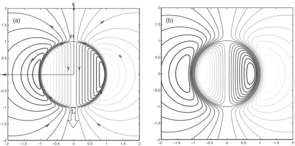
FIG. 6. Typical streamfunction patterns for h = 0.1 (a) and h = 0.4 (b) and a localized Marangoni effect of Gaussian type; w =0.4; µ1=µ2=0.5. The large arrow shows the direction of the net force acting on the drop. As in subsequent figures, dark curves refer to positive values of the streamfunction and therefore clockwise rotating streamlines while light curves refer to negative values of the streamfunction and therefore counter-clockwise rotating streamlines.
−2 −1.5 −1 −0.5 0 0.5 1 1.5 2 −2 −1.5 −1 −0.5 0 0.5 1 1.5 2 y x H L −2 −1.5 −1 −0.5 0 0.5 1 1.5 2 −2 −1.5 −1 −0.5 0 0.5 1 1.5 2 (a) (b)
FIG. 7. Typical streamfunction patterns for h = 0.1 (a) and h = 0.4 (b) and a constant surface tension gradient along x; µ1= µ2=0.5. The H and L labels correspond to the high and low surface tension regions, respectively. The large arrow represents the direction of the total Marangoni force acting on the drop.
while being pushed towards the high surface tension point. In Baroud et al.2and Verneuil et al.,5 such Marangoni-driven flow patterns were observed and the increase of surface tension at the hot point was attributed to surfactant depletion through the laser. The solution for a surface tension deficit at the hot point (as would be expected by a pure thermocapillary effect) is simply obtained by inverting the sign of the arrows on the streamfunction contours, owing to the linearity of the underlying equations.
At this stage, we may check for agreement with the solution of Boos and Thess,11 which is found by retaining only the first mode of the Fourier series (i.e., taking n = 1), shown in Fig.7(note the typographic mistake in their expression (4.22) corresponding to our Eq.(31)). Here, we consider a drop submitted to a constant surface tension gradient ∇γ = ex, i.e., γ = cos (θ ), generated by a
linear temperature or surfactant concentration distribution.
Note that in both the localized and linear heating cases, the result of Boos and Thess11 are recovered, with the variations of the velocities in the radial direction occurring on a length scale imposed by the channel height. In Figures6 and7, this may be inferred from the radial spacing between the streamlines which increases in the case h = 0.4 compared to h = 0.1. The typical length scale in the azimuthal direction, on the other hand, is given by the form of the surface tension variation, determined by w in the case of the Gaussian surface tension distribution and R in the linear case.
V. MODEL VALIDATION
Although the Brinkman equations have been validated for single phase pressure driven flow in high aspect ratio rectangular channels,18the only validation test of the Brinkman equations for the modelling of two-phase flows was conducted, to the authors’ knowledge, by Boos and Thess.11 They considered the flow driven by a one-dimensional constant gradient of surface tension along an infinite flat interface perpendicular to the channel walls and found an analytical solution in the form of a series expansion, as already established by Nadim et al.10They compared the interface velocity obtained by solving Brinkman equations with this exact three-dimensional solution and showed that the agreement improved as the aspect ratio k increased.
Note however that this flow, which is driven by a one-dimensional constant gradient of surface tension along an infinite flat interface, is particular in that the pressure contribution and the viscous normal stress vanish exactly on the interface. The entire flow solution is in fact at constant pressure.
It is therefore natural that a description based exclusively on the tangential shear stress contribution provides the correct force balance on the interface, as noticed by Nadim et al.10These authors further used this observation as the basis of a general expression of the Marangoni force solely based on the tangential shear stress and applied it to the determination of the force acting on a Marangoni-driven drop. We will show that this constitutes an erroneous extrapolation since in these more general geometries, the Marangoni effect generates a pressure field that also contributes to the net force acting on the drop.
Despite this single point of validation, the suitability of the Brinkman model to quantitatively describe surface tension driven phenomena and in particular stress calculations can be questioned since the underlying assumption of scale separation is not verified near the interface. As previ-ously noted by Thompson19considering the flow in a Hele-Shaw cell around a thin solid cylinder, asymptotic matching must be performed between an “outer” flow far from the interface governed by the 2D Darcy equation and an “inner” flow near the interface, which remain inherently three-dimensional.
In the absence of an equivalent analysis for Marangoni flows, and despite recent preliminary attempts,20 we resort to an a posteriori validation of the depth-averaged model: the solution of Brinkman’s equations is compared to the full 3D reference numerical simulation conducted in Sec.III. From first sight, the constant pressure across the channel (Figure4) together with parabolic-like tangential velocity profiles and the extremely small transverse velocity components observed in these 3C-2D Stokes calculations (Figure2), show that the key assumptions underlying Brinkman equations appear to hold for pure Marangoni flow description.
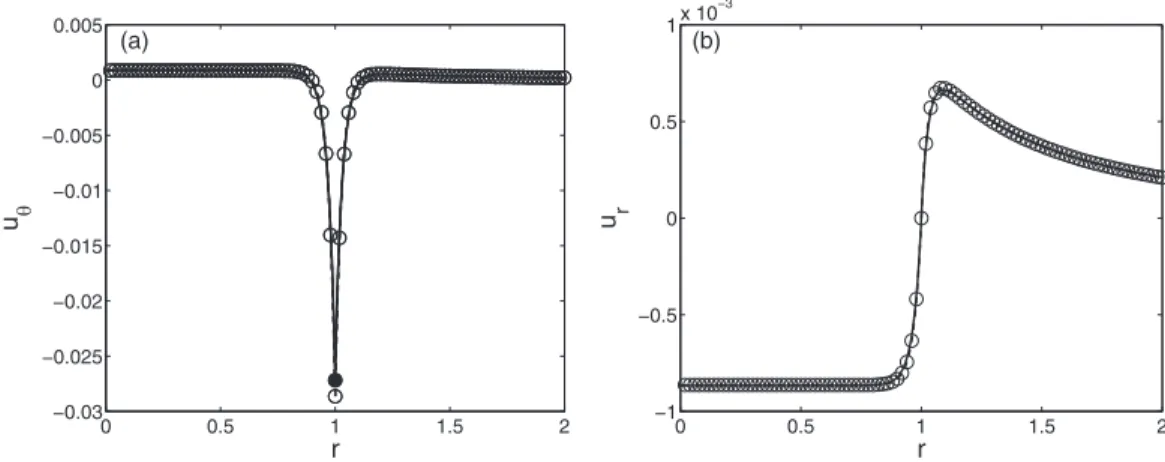
More quantitative comparisons can be obtained by plotting the radial profile of the mean tangential velocity obtained from the Brinkman equations uθ(r, θ = π /2) and the a posteriori depth-average of the 3D Stokes simulations 'Vθ(r, z, θ = π/2)( = 1/ h.
h
z=0Vθ(r, z, θ = π/2)d z, where θ has been set to the arbitrary value of π /2 to factorize out the sinusoidal azimuthal dependence (one has therefore 'Vθ(r, z, θ = π/2)( = 'vθ(r, z)(). As shown in Figure8(a), the overall agreement is remarkable. The estimation given by Nadim et al.,10uNadim
θ (r = 1, θ = π/2) = h 1.842µ
dγ
d x also agrees well with the numerical solution, as shown by the filled circle in Figure 8(a). The radial velocity profile averaged a posteriori in the Stokes simulations and the solution of the Brinkman equations shows the same remarkable agreement (Figure8(b)).
In addition, the shear and normal stresses are compared in Figure 9, displaying a very good agreement. The pressure distribution is particularly well captured, on both sides of the interface, as seen in Figure9(b), where the normal viscous stress contribution is also displayed and seen to be one order of magnitude less than the pressure contribution.
0 0.5 1 1.5 2 −0.03 −0.025 −0.02 −0.015 −0.01 −0.005 0 0.005 r u θ 0 0.5 1 1.5 2 −1 −0.5 0 0.5 1x 10 −3 r u r (a) (b)
FIG. 8. Comparison of the depth-averaged fields resulting from the Stokes simulations (solid lines) and their counterparts directly obtained by solving the Brinkman equations (circles). (a) Radial distribution of the mean tangential velocity 'v(i )θ (r, z)( and the Brinkman solution u(i )θ (r, θ = π/2) (the filled circle denotes the prediction from Nadim’s formula8); (b) Radial distribution of the mean tangential velocity 'vr(i )(r, z)( and the Brinkman solution u(i )r (r, θ = 0); h = 0.1, a1=1, µ1=3/4, and µ2=1/4.
0 0.5 1 1.5 2 −0.8 −0.2 0.4 r τ rθ 0 0.5 1 1.5 2 0 0.1 0.2 0.3 0.4 0.5 0.6 0.7 0.8 r p (a) (b)
FIG. 9. Comparison of the depth-averaged fields resulting from the 3D Stokes simulations (solid lines) and their counterparts directly obtained by solving the Brinkman equations (circles). (a) Radial distribution of the mean tangential shear stress 'tr,θ(i )(r, z)( and the Brinkman solution τ
(i )
r,θ(r, θ = π/2) ; (b) Radial distribution of the mean pressure 'q(i)(r, z)( and viscous normal stress 'tr,r(i )(r, z)( and the respective Brinkman solutions p(i)(r, θ = 0), τr,r(i )(r, θ = 0); h = 0.1, a1=1, µ1=3/4, and µ2=1/4.
Although the presented computations do not bring a mathematical proof of the validity of the Brinkman equations for two-phase flows in Hele-Shaw cells, they may be considered as a reasonable validation of the depth-averaged model, not only as far as the qualitative behavior of the flow is concerned, but also regarding the quantitative pressure and viscous stresses close to the interface. These results also show that the contribution from the pressure field is of comparable magnitude as the tangential stress, as clearly evidenced by comparison of Figures3and4or of Figures9(a) and9(b), while the viscous part of the normal stress on the other hand is one order of magnitude (h/R) smaller. This result has two consequences: (i) the pressure contribution should be included in force calculations on an interface in general, (ii) the determination of this pressure field requires the computation of the full flow field.
VI. FORCE DUE TO THE MARANGONI FLOW
We now wish to evaluate the total force induced by the Marangoni flow on the drop. Three stress terms are exerted by the outer fluid on the cylindrical interface: the pressure field p as well as the viscous shear stresses in the tangential and normal directions, namely, τr θ =µ2
* ∂u(2)r ∂θ + ∂u(2)θ ∂r − u(2)θ r + and τrr =2µ2∂u (2) r
∂r . Another force is applied by the walls onto the drop as a consequence of the friction at the walls, if we consider that the drop is in contact with the plates (wetting drop). If the drop is non-wetting, then the wetting film can be assumed to be thin enough for the shear to be entirely transmitted throughout its negligible thickness, retrieving the previous situation. In any case, the resulting x-component of the total force on the drop is given by the projections of the former three contributions, integrated along the azimuthal direction and the latter contribution integrated on the two circular contact areas between the cylindrical drop and the walls.
The viscous tangential shear force reduces to Ft=µ2h # 2π 0 & −∂u (2) r ∂θ − r ∂u(2)θ ∂r +u (2) θ ' sin(θ )dθ ! ! ! ! !r =1 , (32)
whereas the viscous normal force is recast, using the continuity equation on the drop interface and integrations by parts, as Fn=2µ2h # 2π 0 $ ∂u(2) r ∂θ − u (2) θ % sin(θ )dθ ! ! ! !r =1 . (33)
Similarly, the pressure force is given by Fp=h # 2π 0 − p (2)! !r =1cos(θ )r dθ = h # 2π 0 ∂p(2) ∂θ ! ! ! !r =1 sin(θ )r dθ. (34)
The term ∂p(2)/∂θ may be retrieved from the tangential component of the Brinkman equations µ2 /$ 1 r ∂ ∂rr ∂ ∂r − 1 r2 + 1 r2 ∂2 ∂θ2 − k 2 % u(2)θ + 2 r2 ∂u(2)r ∂θ 0 = 1 r ∂p(2) ∂θ . (35)
The pressure force becomes, after a double integration by parts,
Fp=µ2h # 2π 0 $ 2 r2 ∂u(2) r ∂θ + $ ∂2 ∂r2 + 1 r ∂ ∂r − 2 r2 − k 2 % u(2)θ % sin(θ )r2dθ ! ! ! !r =1 . (36)
Let us now evaluate the viscous friction force of the two plates on the drop
Ff = − # 2π 0 # 1 0 12µ1 h * u(1)r cos(θ ) − u(1)θ sin(θ )+r dθ dr. (37) An integration by parts finally leads to
Ff = −µ1 12 h # 2π 0 r ψ(1)sin(θ )!!r =1dθ. (38)
The final expression for the nondimensional force is obtained by summing the four different contri-butions found in Eqs.(32),(33),(36), and(38), Fm=Ft+Fn+Fp+Ff
Fm=µ2h # 2π 0 $ 3 r2 ∂u(2) r ∂θ + $ ∂2 ∂r2 − k 2 −r32 % u(2)θ − k 2 R2r µ1 µ2 ψ(1) % sin(θ )r2dθ ! ! ! !r =1 . (39)
This expression shows, as a consequence of the orthogonality properties of the sine functions, that only the first component of the Fourier series matters as far as the evaluation of the force is concerned, since all other contributions vanish in the integration once multiplied by sin (θ ). The expressions of AppendixAcan then be used to evaluate the various components of the force
Ft =πhµ2c1 $ 2k K0(k) K1(k) +k2 % , (40) Fn = −πhµ2c1 2k K0(k) K1(k) , (41) Fp =πhµ2c1k2, (42) Ff =0, (43) Fm=2π hµ2c1k2, (44)
where c1is given by Eq.(30).
Note first that Ff=0 as a consequence of the zero average flux in the x direction in the droplet, by construction. Observe also that the normal viscous force Fnis one order of k smaller than the tangential viscous force Ft, as a consequence of the continuity relation ∂∂urr
!
!r =1∼ 1r∂∂θuθ !
!r =1and the separation of scales along the azimuthal and radial directions away from the interface. The above expressions further show that the total force (Fm) is approximately twice as large as the force due to the tangential shear stress (Ft) and exactly twice as large as the result of the total viscous stress (Ft+
Fn) and, equivalently, twice as large as the pressure contribution. Using the asymptotic expansions of(30)and(31)for n = 1, one is led to c1= ak12 + O
(1 k3), which yields Fm≃ 2hµ2 # 2π 0 dγ dθ sin(θ )dθ, (45)
or, in dimensional terms, ¯ Fm≃ 2 ¯h ¯ µ2 ¯ µ1+µ¯2 # 2π 0 dγ¯ dθ sin(θ )dθ. (46)
These forms of the total force may be evaluated for the two cases treated above. For instance, in the case of a temperature induced Gaussian surface tension distribution, as that plotted in Figure6, one finds ¯ Fm≃ − 2√π " ¯T ¯GTh¯w¯µ¯2 ¯ R( ¯µ1+µ¯2) , (47)
in agreement with the scaling law of Baroud et al.2Note the sign of the force which is directed away from the high surface tension region. In the case of a linear surface tension gradient10–12 shown in Figure7, a1=1 and ¯ Fm= −2π ¯h ¯ µ2 ¯ µ1+µ¯2 " ¯T ¯GT, (48)
which is twice the force predicted by Nadim et al.,10who neglected the contribution of the normal stress to the force. Finally, we insist that the linearity of the Stokes equation implies that only the sign of the force will change if the sign of the surface tension dependence on temperature is inverted.
VII. A STATIONARY DROP IN A UNIFORM ADVECTION FLOW
We will now derive the force imposed on a drop by a uniform advection flow of velocity ¯U∞in Hele-Shaw geometry. Recall that we non-dimensionalize the equations with ¯R/ ¯U∞as a time scale and ¯R( ¯µ1+µ¯2) ¯U∞as force scale. The solutions satisfying the far field boundary condition and the regularity condition on the axis may be written as the sum of a potential flow ψparound the drop (and a corresponding velocity field up), violating the continuity of tangential velocity and tangential shear stress along the interface of the drop, and a correction flow of Brinkman’s type which restores this balance ψ(1) =B$ I1(kr ) I1(k) − r % sin(θ ), (49) ψ(2)= $ C$ K1(kr ) K1(k) − 1 r % +ψp % sin(θ ), (50) ψp=r −1 r, (51) B =$ −2µ2(k K1(k) + 2K0(k)) + 4µ2K0(k) d1 % I1(k), (52) C =$ 2µ1(−k I1(k) + 2I2(k)) − 4µ2I2(k) d1 % K1(k), (53)
with d1 given by expression (31). The determination of the constants B and C is the topic of AppendixB. It may be further shown that the asymptotic expansion of C is
C = 2µ1 k + 4 − 9µ1+6µ21 k2 + O $ 1 k3 % . (54)
The amplitude of this constant C has an influence on the typical flow fields, depicted in Figure10. Since C < k−12 at leading order, the radial part of ψ(2) increases monotonically with r. This pre-vents the formation of recirculation zones in the outer fluid that are observed in presence of ad-ditional soluto-capillary flow.12Since up
r ! !r =1 =0, u p θ ! !r =1= −2 sin(θ), and ∂2up θ ∂r2 ! ! !r =1= −6 sin(θ),
−2 −1.5 −1 −0.5 0 0.5 1 1.5 2 −2 −1.5 −1 −0.5 0 0.5 1 1.5 2 y x −2 −1.5 −1 −0.5 0 0.5 1 1.5 2 −2 −1.5 −1 −0.5 0 0.5 1 1.5 2 (a) (b)
FIG. 10. Typical streamfunction patterns for h = 0.1 (a) and h = 0.4 (b) in presence of an outer uniform flow; µ1=µ2= 0.5. The large arrow represents the net force, which is due to the drag acting on the drop.
plugging-in the flow fields of Eq.(50)into the general expression for the force(39)yields the force F∞that acts on the drop owing to the external flow
F∞=πhµ22k2(1 + C). (55)
Using the asymptotic estimate(54)yields a dimensionless drag force, at leading order F∞≃ πhµ22k2 $ 1 +2µ1 k + 4 − 9µ1+6µ21 k2 % . (56)
This expression shows that taking into account the tangential stress condition along the interface increases the drag force on the drop or bubble by two lower order terms in comparison to the case of a solid disk ( ¯F∞=24π ¯U∞µ¯2
¯ R2
¯
h ). Note that at fixed outer viscosity ¯µ2, the drag force is an increasing function of the inner viscosity.
The linearity of the Stokes equation enables one to determine the incoming velocity at which the drag force and the Marangoni force exactly balance by simply adding up the solution for a stationary droplet in uniform flow to the solution for the Marangoni induced flow derived previously. At leading order, the total force becomes
¯ F ≃ ¯µ2U¯∞π2k2h − 2 ¯h¯ ¯ µ2 ¯ µ1+µ¯2 # 2π 0 "γ¯dγ dθ sin(θ )dθ. (57)
The drop therefore remains stationary in the oncoming stream of speed ¯U∞if # 2π 0 "γ¯dγ dθ sin(θ )dθ = k 2 ¯ U∞π( ¯µ1+µ¯2). (58)
It is important to note here that while the global force balance is ensured, it can be shown that the local normal stress balance is not satisfied, even in the situation of a linear surface tension gradient. This contrasts with the “unique” situation15 of spherical droplets in unbounded flows, suggesting that actual pancake droplets held by a surface tension gradient against the flow in a Hele-Shaw cell will deform.
Typical flow fields of a drop in a uniform flow counterbalanced by a localized surface tension gradient are depicted in Figure 11. This flow field compares favourably with the experimental streamlines observed by Baroud et al.2and Verneuil et al.5inside and outside the droplet (in these experiments, the flow along the interface was directed towards the focal point of the laser, where the local surface tension increase was caused by the depletion of surfactant molecules from the water-oil
−2 −1.5 −1 −0.5 0 0.5 1 1.5 2 −2 −1.5 −1 −0.5 0 0.5 1 1.5 2 y x H L −2 −1.5 −1 −0.5 0 0.5 1 1.5 2 −2 −1.5 −1 −0.5 0 0.5 1 1.5 2 (a) (b)
FIG. 11. Typical streamfunction patterns for h = 0.1 (a) and h = 0.4 (b) for a drop held stationary in a constant outer flow with localized surface tension gradient; ¯w =0.4; µ1=µ2=0.5.
−2 −1.5 −1 −0.5 0 0.5 1 1.5 2 −2 −1.5 −1 −0.5 0 0.5 1 1.5 2 y x H L −2 −1.5 −1 −0.5 0 0.5 1 1.5 2 −2 −1.5 −1 −0.5 0 0.5 1 1.5 2 (a) (b)
FIG. 12. Typical streamfunction patterns for h = 0.1 (a) and h = 0.4 (b) for a drop held stationary in an outer flow through a linear surface tension gradient; µ1=µ2=0.5.
interface5). In doing so, the Marangoni flow significantly modifies the streamlines, entraining fluid that was originally far from the drop into the hot region, as shown in Fig.11. This leading-order modification of the flow field can have a significant effect on the transport of solutes in the outer flow, as well as the transport of surfactant molecules along the surface of the drop, as long as the solutal Peclet number is non-zero.
The case of a constant surface tension gradient holding a drop stationary is shown in Figure12. The addition of the Marangoni flow causes the outer streamlines to become straight, giving the impression that the drop becomes “cloaking” to the flow in the far-field.
VIII. TRANSLATING DROPLETS
With these expressions at hand, it is tempting to apply them to moving droplets translating at a typical velocity ¯Ud. Although such an approach has been followed by Taylor and Saffmann,21 Nadim et al.,10 and Bush12 among others, it hinges onto dynamic contact line issues for wetting droplets and the presence of curved dynamic wetting films for non-wetting droplets.
In this latter case, it is known since Bretherton,22Foster and Burgess,23and Park and Homsy24 that viscous dissipation in the dynamic meniscus region induces a second source of drag on a moving drop, that scales like ¯Fca ∼ ¯γ ¯RCa2/3, where the capillary number Ca is defined as Ca = µ¯2
¯ Ud ¯ γ . This scaling can be obtained by a Landau-Levich type balance between capillary and viscous forces in the thin films that lubricate the drop motion. The relative strength of ¯Fca with respect to the forces that can be calculated by neglecting the thin films ¯FD∼ ¯h ¯µ2U¯dπk2is given by ¯Fca/ ¯FD∼ Ca−1/3k, showing that, despite the vanishing thickness of the capillary films, their contribution to the drag forces dominates at low capillary numbers.24
This dynamic wetting film effect, associated to the curvature variations in the dynamic meniscus regions, cannot be modelled in the present depth-averaged approach assuming a frozen flattened circular cylindrical interface. Still, for the purpose of comparison with previous findings10,12,21and with these strong limitations in mind, we now turn to the case of translating droplets.
A. Translating drop in a quiescent outer fluid
Let us embark in the reference frame of the lab with fixed walls and consider a translating drop at velocity − ¯Ud in a stationary outer fluid. Using a similar method, it can be shown that the flow becomes ψ(1)= $ B′$ I1(kr ) I1(k) − r % − r % sin(θ ), (59) and ψ(2)= $ C′$ K1(kr ) K1(k) − 1 r % −1r % sin(θ ), (60) with B′=$ −2µ2(k K1(k) + 2K0(k)) + (3µ2+µ1)K0(k) d1 % I1(k), (61) C′=$ 2µ1(−k I1(k) + 2I2(k)) − (3µ2+µ1)I2(k) d1 % K1(k), (62)
as detailed in AppendixC. Typical flow fields in the reference frame of the laboratory are depicted in Figure13. −2 −1.5 −1 −0.5 0 0.5 1 1.5 2 −2 −1.5 −1 −0.5 0 0.5 1 1.5 2 y x −2 −1.5 −1 −0.5 0 0.5 1 1.5 2 −2 −1.5 −1 −0.5 0 0.5 1 1.5 2 (a) (b)
FIG. 13. Typical streamfunction patterns for h = 0.1 (a) and h = 0.4 (b) for a drop translating downwards, shown in the reference frame of the laboratory; µ1=µ2=0.5. The arrow shows the direction of the net force due to the drag force.
Since ∂urpot ∂θ ! ! !r =1=sin θ , ψ (1)| r =1= −sin (θ), u pot θ ! !r =1= − sin(θ) and ∂2upot θ ∂r2 ! ! !r =1= −6 sin(θ), inserting Eqs.(59)and(60)into the general expression for the force(39)yields
Fd =µ2hπ(2C′k2+k2) + hk2πµ1, (63)
which gives, using C′= 2µ1 k + 3−7µ1+6µ21 k2 + O (1 k3) , Fd ≃ πhµ2k2 $ 1 +4µ1 k + 6 − 14µ1+12µ21 k2 % +πhµ1k2. (64)
This expression, once made dimensional, becomes ¯ Fd = ¯hµ¯2U¯dπk2+ ¯hµ¯1U¯dπk2+ ¯h 4 ¯µ2µ¯1 ¯ µ1+µ¯2 ¯ Udπk + O(1). (65)
It may be compared at leading order to expression (32) of Nadim et al.10 The first two terms correspond exactly to their findings while the third one, though of the correct order of magnitude reveals a discrepancy in the prefactor, since ours is√12/1.842 ≈ 1.9 larger. Similar to the pure Marangoni flow described in Sec.VI, the Brinkman model takes into account the pressure correction caused by imposition of the depth-averaged tangential velocity and stress continuities, which is neglected by Nadim et al.10
B. Translating drop in a uniform flow
As a next application of the flow patterns and forces derived in this section, let us now con-sider a moving drop at velocity ¯Ud in an outer stream of velocity ¯U∞. Linear superposition of Eqs.(56)and(65)yields
¯
F ≃(2 ¯µ2U¯∞− ( ¯µ1+µ¯2) ¯Ud) πk2h.¯ (66) In the case of a gas bubble ( ¯µ1≪ ¯µ2), the dynamical equilibrium is reached when
¯
Ud =2 ¯U∞, (67)
recovering the famous result of Taylor and Saffman21by an alternative method. C. Marangoni-driven self-propelled drop in a quiescent outer fluid
The next application considered is that of a Marangoni-driven self-propelled drop either is a constant surface tension gradient, a situation widely discussed in square and round capillaries,25,26 or in a more general surface tension distribution. Combining the drag force(65)and the Marangoni driving force(46), one is led to
¯ F = ¯h( ¯µ2+µ¯1) ¯Udπk2+4 ¯h ¯ µ2µ¯1 ¯ µ1+µ¯2 ¯ Udπk − 2 ¯h ¯ µ2 ¯ µ1+µ¯2 # 2π 0 dγ¯ dθ sin(θ )dθ. (68)
The cancellation of the force gives the final velocity of the drop, ¯ Ud= − 2 ¯µ2 .2π 0 γ¯cos(θ )dθ π(k2( ¯µ 1+µ¯2)2+4k ¯µ2µ¯1 ) , (69)
to be compared with the prediction of Nadim et al.10 ¯ UNadim= − ¯ µ2. 2π 0 γ¯cos(θ )dθ π * k2( ¯µ 1+µ¯2)2+4k ¯µ2µ¯1 √ 12/1.842+ . (70)
The two differences with the expressions of Nadim et al.10already found in expressions(46)and(65) are combined in the resulting expression for the terminal velocity. Typical streamlines of these compound flows are depicted in Figures14and15.
−2 −1.5 −1 −0.5 0 0.5 1 1.5 2 −2 −1.5 −1 −0.5 0 0.5 1 1.5 2 y x H L −2 −1.5 −1 −0.5 0 0.5 1 1.5 2 −2 −1.5 −1 −0.5 0 0.5 1 1.5 2 (a) (b)
FIG. 14. Typical streamfunction patterns for h = 0.1 (a) and h = 0.4 (b) of a translating drop propelled by a following localized Marangoni force; ¯w =0.4; µ1=µ2=0.5.
D. Marangoni retardation of buoyancy driven droplets
In the case of a gas bubble, ¯µ1=0 and a constant retarding surface tension gradient, Eq.(64) yields ¯ F = ¯hµ¯2U¯dπk2+6 ¯hµ¯2U¯dπ − 2 ¯h # 2π 0 dγ¯ dθ sin(θ )dθ, (71)
introducing the notation of Bush12T = "γ¯ ¯ µ ¯Ud ¯ F = ¯hµ¯2U¯dπ(k2+(6 + 2T )) . (72) −2 −1.5 −1 −0.5 0 0.5 1 1.5 2 −2 −1.5 −1 −0.5 0 0.5 1 1.5 2 −2 −1.5 −1 −0.5 0 0.5 1 1.5 2 −2 −1.5 −1 −0.5 0 0.5 1 1.5 2 y x H L (a) (b)
FIG. 15. Typical streamfunction patterns for h = 0.1 (a) and h = 0.4 (b) of a translating drop propelled by a constant surface tension gradient; µ1=µ2=0.5.
Balancing this drag force with a buoyancy force in an inclined Hele-Shaw cell yields the terminal velocity ¯ Ud ≃ ¯ h2g¯sin(α) 12 ¯µ2 (1 − (6 + 2T )/k 2) (73) whereas Eq. (5.23) of Bush12yields
¯ UBush≃ ¯ h2g¯sin(α) 12 ¯µ2 (1 − (2 + T )/k 2) . (74) It should be noted that we obtain the same scalings as Bush12 by a completely different method, with a different prefactor however. We may speculate that this discrepancy could be related to the asymptotic expansions used by Bush12for the domain integration of the viscous dissipation around the bubble, whereas the present analysis makes use of the exact Bessel functions.
IX. SUMMARY AND DISCUSSION
In summary, we have proposed a thorough analysis of Marangoni induced forces on drops in a Hele-Shaw geometry. The decomposition of the flow field into Fourier modes provides a standard method to solve for the streamfunction and the forces in a general context, as long as the form of the surface tension profile is known. This analysis unifies the two approaches of Nadim et al.,10 Boos and Thess,11and Bush12through a rigorous approach analogous to the analysis of a spherical drop of Hadamard13and Rybzynski.14
Two characteristic cases were studied in detail: (i) that of a localized forcing which might correspond to heating from a laser source or a local variation of surfactant concentration and (ii) the more classical case of a constant temperature gradient. The extension of the method presented here to any Marangoni stress is straight-forward.
With thermocapillary applications in mind, one may ask what typical temperature distribution is the most efficient to block a drop. Examination of Eq.(47)shows that for the same maximum temperature difference "T, Fmscales like w implying that the strength of the force increases with the width of the hot spot. For a fixed laser power P however, assuming that the hot spot size w scales like the laser width, "T ∝πwP2 and the resulting force is inversely proportional to the spot width.
This suggests that a tighter laser focusing leads to an increased blocking efficiency. This result is consistent with the measurements of the dependence on beam waist discussed in Baroud et al.3and Verneuil et al.5
For a typical microfluidic application, consider the case of a water drop of radius 150 µm and height 50 µm, with a maximum surface tension difference of 25 mN/m. Using the viscosities of water (µ1 =10−3 Pa s) and hexadecane as the external fluid (µ2 ≃ 3 × 10⁻³ Pa s) and taking w =50 µm, we may calculate the forces acting on the drop. The Marangoni force due to a localized forcing may be evaluated from Eq.(47)as Fm≃ 10−6 N, showing that the characteristic forces are on the order of a micro-Newton. In the same conditions, the drag force caused by a uniform stream at 1 cm/s may be evaluated from the dimensional version of Eq.(56)given at leading order by F∞=24πU µ2R
2
h to also be on the order of a micro-Newton, indicating that the drop can be stopped under these conditions.
The equilibria calculated above all hinge on assuming a circular drop in an infinite medium, which allows analytical solutions to be found. In practical situations however, the actual shape of the drop will be governed by the presence of walls and shear flows and these departures from circularity and confinement will alter the relative contributions of the stress fields. In particular, Verneuil et al.5 measured the force acting on a drop simultaneously with the internal velocity field. The values of the interface velocity were found to be insufficient to account for the magnitude of the net force, a result that was attributed to the confinement within the microchannel, since the shear stress between the elongated drops and the lateral walls was found to provide a source for the observed force magnitudes.
This experiment motivates the development of numerical methods for solving Brinkman’s equations in complex geometries. As the value of the capillary number is increased further, the drop
shape will significantly depart from circularity and this will couple back to the flow fields. Further refinement of the model will need to be made to account for these shape variations.
As discussed in Sec. VIII, further extensions of the model should take into account finite capillary number effects when droplets are translating, including the significant curvature imbalance between the advancing and receding menisci for non-wetting droplets and contact angle hysteresis for the wetting case.
Finally, the transport of solutes can also be determined from the knowledge of flow fields. In the case of active molecules such as surfactants, this transport will feed back on the surface tension distribution. Future numerical solutions of these coupled problems will allow quantitative predictions on microfluidic thermocapillary manipulations.
As a last word of caution, it should be mentioned that Lee et al.20 have recently observed experimentally strong deviations from parabolic profiles in the vicinity of the interface using a geometrical anchor holding the droplet in place.27 Such a situation, in which Brinkman equations are likely to become invalid, was observed to happen when the Marangoni effect was pulling on the interface in the opposite direction as that of the carrier flow, which fundamentally differs from the presently considered case where the surface tension gradient pushes the fluid in the direction of the external flow, as required by the zero force balance.
ACKNOWLEDGMENTS
The authors acknowledge the help of J. P. Delville in initiating this work and useful discussions with G. Iooss and R. Dangla. P. Laure thanks the team CIM for providing their finite element Library (http://www.cemef.mines-paristech.fr/). F. Gallaire acknowledges the support of ERC grant SIMCOMICS.
APPENDIX A: MARANGONI FLOW
Starting with streamfunctions of the form given in Sec.III ψ(2)= ∞ " n=1 cn $ Kn(kr ) Kn(k) − 1 rn % sin(nθ ), (A1) ψ(1)= ∞ " n=1 bn $ In(kr ) In(k) − r n % sin(nθ ), (A2)
the tangential velocities are easily expressed u(2)θ = ∞ " n=1 cn $ −K ′ n(kr ) Kn(k) − n rn+1 % sin(nθ ), (A3) u(2)θ = ∞ " n=1 cn $ kKn−1(kr ) Kn(k) +n r Kn(kr ) Kn(k) − n rn+1 % sin(nθ ), (A4) u(1)θ = ∞ " n=1 bn $ −I ′ n(kr ) In(k) +nrn−1 % sin(nθ ), (A5) u(1)θ = ∞ " n=1 bn $ −kIn+1(kr ) In(k) − n r In(kr ) Kn(k) +nrn−1 % sin(nθ ). (A6)
The radial velocities are
u(2)r = ∞ " n=1 cn $ n r Kn(kr ) Kn(k) − n rn+1 % cos(nθ ), (A7) u(1)r = ∞ " n=1 bn n r $ In(kr ) In(k) − nr n−1 % cos(nθ ), (A8)
retrieving the pressure µ2 /$ 1 r ∂ ∂rr ∂ ∂r − 1 r2 + 1 r2 ∂2 ∂θ2 − k 2 % u(2)θ + 2 r2 ∂u(2)r ∂θ 0 =1 r ∂p(2) ∂θ , (A9) µ2 /$ 1 r ∂ ∂r + ∂2 ∂r2 − 1 r2 + 1 r2 ∂2 ∂θ2 − k 2 % u(2)θ + 2 r2 ∂u(2)r ∂θ 0 = 1 r ∂p(2) ∂θ , (A10) requires ∂u(2)θ ∂r = ∞ " n=1 cn $ −k2KKn(kr ) n(k) − k r Kn−1(kr ) Kn(k) − n(n + 1) r2 Kn(kr ) Kn(k) +n(n + 1) rn+2 % sin(nθ ), (A11) ∂2u(2)θ ∂r2 = ∞ " n=1 cn $ k3Kn−1(kr ) Kn(k) +(n + 1)k 2 r Kn(kr ) Kn(k) +(n 2+ 2)k r2 Kn−1(kr ) Kn(k) (A12) +n(n + 1)(n + 2) r3 Kn(kr ) Kn(k) − n(n + 1)(n + 2) rn+3 % sin(nθ ), ∂u(1)θ ∂r = ∞ " n=1 bn $ −k2IIn(kr ) n(k) +k r In+1(kr ) In(k) − n(n − 1) r2 In(kr ) In(k) +n(n − 1)rn−2 % sin(nθ ), (A13) ∂2u(1)θ ∂r2 = ∞ " n=1 bn $ −k3In+1(kr ) In(k) − (n − 1)k2 r In(kr ) In(k) − (n2+2)k r2 In+1(kr ) In(k) (A14) −n(n − 1)(n − 2)r3 In(kr ) In(k) +n(n − 1)(n − 2)rn−3 % sin(nθ ), and the associated shear stresses are given by
∂u(2)θ /r ∂r = ∞ " n=1 cn $ 1 r K′ n(kr ) Kn(k) + n rn+2 − K′′ n(kr ) Kn(k) +n(n + 1) rn+2 % sin(nθ ), (A15) ∂u(2)θ /r ∂r = ∞ " n=1 bn $ 1 r In′(kr ) In(k) − nr n−2−In′′(kr ) In(k) +n(n − 1)rn−2 % sin(nθ ). (A16)
Imposing the continuity of tangential velocity as well as the Marangoni shear stress discontinuity yields as boundary conditions
bn $ −I ′ n(k) In(k) +n % =cn $ −K ′ n(k) Kn(k) − n % , (A17) µ1bn $ I′ n(k) In(k)− I′′ n(k) In(k) +n(n − 2) % − ¯µ2cn $ K′ n(k) Kn(k) − K′′ n(k) Kn(k) +n(n + 2) % =an. (A18)
Using the following Bessel relations:
In(kr )′=k In+1(kr ) + n rIn(kr ), (A19) Kn(kr )′= −k Kn−1(kr ) − n rKn(kr ), (A20) In(kr )′′=k2In(kr ) − k rIn+1(kr ) + n(n − 1) r2 In(kr ), (A21) Kn(kr )′′=k2Kn(kr ) + k rKn−1(kr ) + n(n + 1) r2 Kn(kr ), (A22)
the 2 × 2 linear system becomes −k In+1(k)/In(k) −k Kn−1(k)/Kn(k) ¯ µ1(−k 2I n(k)+2k In+1(k) In(k) ) µ2( k2K n(k)+2k Kn−1(k) Kn (k)) & bn cn ' = & 0 an ' , (A23) or in synthetic form Mn & bn cn ' = & 0 an ' . (A24)
The solution of this system is then given by $ bn cn % = & K n−1(k)an dn −In+1(k)an dn ' (A25) with dn= −µ2In+1(k)(k2Kn(k) + 2k Kn−1(k)) + µ1Kn−1(k)(−k2In(k) + 2k In+1(k)) . (A26) Now specifying to the case n = 1, all the necessary expressions required for the determination of the forces are obtained
u(2)θ = c1 K1(k) $ k K0(kr ) + K1(kr ) r − K1(k) r2 % sin(θ ), (A27) ∂u(2)θ ∂r = − c1 K1(k) $ k2K1(kr ) + k K0(kr ) r + 2K1(kr ) r2 − 2K1(k) r3 % sin(θ ), (A28) ∂2u(2)θ ∂r2 = c1 K1(k) $ k3K0(kr ) + 2k2K1(kr ) r + 3k K0(kr ) r2 + 6K1(kr ) r3 − 6 K1(k r4 % sin(θ ). (A29) Their evaluation on the boundary yields
u(2)θ ! ! !r =1= c1k K0(k) K1(k) sin(θ ), (A30) ∂u(2)θ ∂r ! ! ! ! !r =1 = −c1(k 2K 1(k) + k K0(k)) K1(k) sin(θ ), (A31) ∂2u(2)θ ∂r2 ! ! ! ! !r =1 = c1(k 3K 0(k) + 2k2K1(k)) + 3k K0(k) K1(k) sin(θ ). (A32)
APPENDIX B: STATIONARY DROP IN UNIFORM FLOW
As detailed in Sec.V, the solutions satisfying the far field boundary condition and the regularity condition on the axis are
ψ(1)= $ Ar + BI1(kr ) I1(k) % sin(θ ), (B1) ψ(2)= $ D/r + r + CK1(kr ) K1(k) % sin(θ ). (B2)
The boundary condition ψ(1)=ψ(2)=0 yields
The flow therefore appears as the sum of a Marangoni flow, similar to that studied in AppendixA, and a potential flow
ψ(1) =B$ I1(kr ) I1(k) − r % sin(θ ), (B4) ψ(2)= $ C$ K1(kr ) K1(k) − 1 r % +ψp % sin(θ ), (B5) with ψp=r −1 r. (B6) Since uθp= $ 1 + 1 r2 % sin(θ ) and r∂u p θ/r ∂r = $ −1r −r33 % sin(θ ), (B7)
B and C are given by the two remaining boundary conditions, i.e., the continuity of tangential velocity and tangential shear stress, by a linear system analogous to the one solved in AppendixA with a different R.H.S., M1 $ B C % =$ −2 4µ2 % . (B8)
The solution of this system is
B =$ −2µ2(k K1(k) + 2K0(k)) + 4µ2K0(k) d1 % I1(k), (B9) C =$ 2µ1(−k I1(k) + 2I2(k)) − 4µ2I2(k) d1 % K1(k). (B10)
APPENDIX C: TRANSLATING DROP
When a translating drop is considered as in Sec.VI, one gets similarly M1 $ B′ C′ % = $ −2 3µ2+µ1 % . (C1)
The solution of this system is
B′=$ −2µ2(k K1(k) + 2K0(k)) + (3µ2+µ1)K0(k) d1 % I1(k), (C2) C′=$ 2µ1(−k I1(k) + 2I2(k)) − (3µ2+µ1)I2(k) d1 % K1(k). (C3)
1A. Darhuber and S. Troian, “Principles of microfluidic actuation by modulation of surface stresses,”Annu. Rev. Fluid Mech.37, 425–455 (2005).
2C. Baroud, J.-P. Delville, F. Gallaire, and R. Wunenburger, “Thermocapillary valve for droplet production and sorting,” Phys. Rev. E75, 046302 (2007).
3C. Baroud, M. de Saint Vincent, and J.-P. Delville, “An optical toolbox for total control of droplet microfluidics,”Lab Chip
7, 1029–1033 (2007).
4M. Cordero, D. Burnham, C. Baroud, and D. McGloin, “Thermocapillary manipulation of droplets using holographic beam shaping: Microfluidic pin ball,”Appl. Phys. Lett.93, 034107 (2008).
5E. Verneuil, M. Cordero, F. Gallaire, and C. Baroud, “Anomalous thermocapillary force on microdroplet: Origin and magnitude,”Langmuir25, 5127–5134 (2009).
6K. Kotz, K. Noble, and G. Faris, “Optical microfluidics,”Appl. Phys. Lett.85, 2658–2660 (2004).
7R. Grigoriev, M. Schatz, and V. Sharma, “Chaotic mixing in microdroplets,”Lab Chip6, 1369–1372 (2006).
8N. Young, J. Goldstein, and M. Block, “The motion of bubbles in a vertical temperature gradient,”J. Fluid Mech.6, 350–356 (1959).