Quelques propriétés d’un estimateur à noyau du
quantile conditionnel pour des données associées
Some properties of a kernel conditional quantile estimator for
associated data
Latifa Adjoudj1, Abdelkader Tatachak1
1Laboratory MSTD, USTHB, Algiers, Algeria, ladjoudj@usthb.dz, atatachak@usthb.dz
RÉSUMÉ. Le présent article vise à établir certaines propriétés asymptotiques d’estimateurs à noyau de la fonction de distribution conditionnelle et du quantile conditionnel lorsque les observations de durée de vie et les covariables sont associées.
ABSTRACT. This paper aims to establish some asymptotic properties of kernel estimators of the conditional distribution function and the conditional quantile when the lifetime observations and the covariates are associated.
MOTS-CLÉS. Association, estimateur à noyau, consistance uniforme forte, quantile conditionnel. KEYWORDS. Association, conditional quantile, kernel estimator, strong uniform consistency.
Introduction
The study of conditional quantile functions is appealing for a number of reasons, particularly because it provides a more comprehensive picture of the conditional distribution of a dependent variable than traditional regression that restricts attention to the conditional mean function only. It is well known that the quantile function can give a good description of the data, see [CHAUDHURI et al. 1997]. An impor-tant application of conditional quantiles is that they provide reference curves or surfaces and conditional prediction intervals that are widely used in many different areas, for example :
− Medicine : reference growth curves for children’s height and weight as a function of age ; − Economics : reference curves to study discrimination effects and trends in income inequality ; − Ecology : to observe how some covariates can affect limiting sustainable population size ; − Lifetime analysis : to assess influence of risk factors on survival curves.
A vast literature is dedicated to the nonparametric estimation of conditional quantile.To quote only a few of them, we recall that [MEHRA et al. 1991] and [XIANG 1996] gave the almost sure (a.s.) convergence of a kernel type conditional quantile estimator and its asymptotic normality. [HONDA 2000] dealt with
α−mixing processes and proved the uniform convergence and asymptotic normality using the local
po-lynomial fitting method.
Here, we are interested in studying another type of dependence, called association. Recall that real-valued
random variables (rv’s) {Zi; 1 ≤ i ≤ N} which are defined on a common probability space (Ω, A , P)
are said to be associated if for every pair of functions h1, h2 : RN → R, which are coordinate-wise
non-decreasing and for whichE[h2k(Zi, 1 ≤ i ≤ N) ]
<∞ ; k = 1, 2, it holds that :
cov (h1(Zi, 1 ≤ i ≤ N), h2(Zj, 1≤ j ≤ N)) ≥ 0.
In classical statistical inference, the rv’s of interest are generally assumed to be iid. However, it is more common to have dependent variables in some real life situations. Dependent variables are present in several backgrounds such as medicine, biology and social sciences. The notion of association was firstly introduced by [ESARY et al. 1967] mainly for an application in reliability. For more details on the subject
we refer the reader to the monographs by BULINSKI and SHASHKIN 2007], [OLIVEIRA 2012] and [PRAKASA RAO 2012].
Let (X, Y ) ∈ Rd × R, for which there exist a common unknown joint distribution function (df) F (·, ·) and marginals FX(·) and FY(·). In what follow we will denote by v(x), F (·|x) and f(·|x) the probability density function (pdf) of the covariate X, the conditional df and the conditional pdf of Y given X = x,
respectively. The conditional df of Y given X = x is F (y|x) = E (1Y≤y|X = x) (where 1A is the
indicator function of the set A) which we reformulate as follows :
F (y|x) = F1(x, y) v(x) := 1 v(x) × ∂F (x, y) ∂x . [1]
Traditionally, a natural estimator of F (·|x) is the empirical conditional df FN(·|x), while the
estima-tion of the p-th condiestima-tional quantile qp(x) := inf{y ∈ R : F (y|x) ≥ p}, p ∈ (0, 1) is done via
qp,N(x) = inf{y ∈ R : FN(y|x) ≥ p}.
Here, we assume that{(Xi, Yi); 1 ≤ i ≤ N} forms a strictly stationary sequence of associated random vectors distributed as (X, Y )∈ Rd× R.
The paper is organized as follows. In Section 1, we recall the notations and the definition of our es-timators. The main results and the assumptions are listed in Section 2. In Section 3, we evaluate the performance of the estimator on simulated data. The proofs of the results are relegated to Section 4.
1. Notation and estimates
estimation of the conditional df”s is based on the choice of weights. The traditional kernel estimator of F (y|x) is given by FN(y|x) =
∑N
i=1wi,N(x)1Yi≤y, where wi,N(.) are measurable functions. These
weights were introduced by Nadarya-Watson and defined by
wi,N(x) = Kd ( x−Xi hN,K ) ∑N i=1Kd ( x−Xi hN,K ) = 1 (N hd N,K) Kd ( x−Xi hN,K ) vN(x) ,
with the convention 00 = 0, and where
vN(x) = 1 N hd N,K N ∑ i=1 Kd ( x− Xi hN,K ) , [2]
is the classical Parzen-Rosenblatt estimator for v. Here Kd : Rd → R+ is a multivariate kernel such that for any zℓ = (z1ℓ, z2ℓ, . . . , zℓd)⊤ ∈ Rdand a real-valued univariate kernel K
1 hdN,KKd ( zℓ hN,K ) := d ∏ k=1 1 hN,K K ( zℓk hN,K ) .
Furthermore,{hN,K} is a sequence of positive constants tending to zero when N tends to infinity, called
a bandwidth sequence. Here, hN,K is assumed to be the same regardless of the k-th direction. However,
Let us define an estimator for f (y|x) as follows :
fN(y|x) =
fN(x, y)
vN(x) 1{vN(x)̸=0}
with fN(x, y) = 1 N hN,HhdN,K N ∑ i=1 Kd ( x− Xi hN,K ) H(1) ( y− Yi hN,H ) . [3]
Here H(1)(·) denotes a positive kernel function defined on R and ∫−∞y H(1)(z)dz =: H(y) is a df. The
sequences{hN,K} =: hK and {hN,H} =: hH are positive bandwidths that decrease to zero along with
N . Now, in view of (1) we have
f (x, y) = ∂F1(x, y) ∂y ,
hence from (3) one may define an estimator for F1(x, y) as
F1,N(x, y) = 1 N hHhdK N ∑ i=1 Kd ( x− Xi hK ) ∫y −∞ H(1) ( t− Yi hH ) dt = 1 nhdK N ∑ i=1 Kd ( x− Xi hK ) H ( y− Yi hH ) . [4]
So, the estimators in (2) and (4) enable to derive an estimator for F (y|x), that is
FN(y|x) =
F1,N(x, y)
vN(x) 1{vN(x)̸=0}
. [5]
Note that the formulation of the estimator in (5) was introduced by [YU and JONES 1998] as an alter-native to the so-called adjusted Nadaraya-Watson estimator of the conditional df. The main motivation was to overcome the crossing problem associated with the kernel weighting estimation when using the indicator function instead of a continuous df.
So, for a fixed x ∈ Rd and p ∈ (0, 1), a natural estimator (say, qp,N(x)) of the p-th conditional quantile can then be defined as
qp,N(x) = inf{y ∈ R : FN(y|x) ≥ p}.
2. Main results
Let Ω0 and [a, b] be two compact subsets of Γ0 = {x ∈ Rd; inf
x v(x) =: γ > 0} and R respectively.
And let us define
ηij := d ∑ k=1 d ∑ ℓ=1 cov(Xik, Xjℓ) + 2 d ∑ k=1 cov(Xik, Yj) + cov(Yi, Yj), [6]
where Xik is the k-th component of Xi; k = 1, 2, . . . , d.
In what follow the letter C will denote a finite positive constant which is allowed to change from line to line.
2.1. Assumptions
(H1) For all d≥ 1 and β ∈ (0, 1), the bandwidths satisfy
(i) hK → 0, Nh d(1−β)+2β K → ∞ and log5N N hd K → 0 as N → ∞ ; (ii) hH → 0, NhHhdK → ∞ as N → ∞ ;
(H2) The kernel Kdsatisfies
(i) Kd is a bounded pdf, compactly supported and Hölder continuous with exponent β;
(ii)∫RdzkKd(z)dz = 0 for k = 1, . . . , d.
(H3) The df H(·) is compactly supported, continuously differentiable and its derivative H(1)is a second-order kernel.
(H4) For all i≥ 1, the covariance term in (6) satisfies sup
j:|i−j|≥s
ηij =: ρ(s)≤ τ0e−τs; for some positive constants τ0, τ and s.
(H5) The pdf v(·) is bounded and satisfies sup
x∈Ω0 ∂x∂km∂xv(x)m−1 l ≤ C for k,l = 1,... ,d and m = 1,2. (H6) For all integers j ≥ 1, the joint conditional pdf vj(·, ·) of (X1, X1+j) exists and satisfies
sup
(r,s)∈Ω2 0
|vj(r, s)| ≤ C.
(H7) The joint pdf f (·, ·) of (X, Y ) is bounded and twice continuously differentiable.
(H8) For all integers j ≥ 1, the joint conditional fj(·, ·, ·, ·) of (X1, Y1, X1+j, Y1+j) exists and satisfies
sup
(r,u),(s,t)∈{Ω0×[a,b]}2
fj(r, u, s, t) ≤ C.
2.1.1. Comments on the assumptions
(H1) and (H2)-(H3) are quite usual in kernel estimation setting. Note that the sequences {hK} and
{hH} in (H1) are not generally equal as it will be seen in the simulations, while several papers suppose their equality to simplify computations. In addition, in view of nhHhdK → ∞ in (H1)(ii), the condition
nhd(1K −β)+2β → ∞ in (H1)(i) becomes superfluous as soon as d ≥ 2 or for all d ≥ 1 provided hH ≤ hβK (β is that in (H2(i)). Thus, (H1)(i) is only useful in the case d = 1 and hH > hβK. Assumption (H4) quantifies a progressive tendency from dependence to asymptotic independence between "past" and "fu-ture". This latter condition was made in Doukhan and Neumann (2007) in order to state an exponential inequality which we apply to prove Proposition 1 hereinafter.
Assumptions (H5)-(H8) are needed in bias and covariance computation.
2.2. Strong uniform consistency
PROPOSITION 1– Under assumptions (H1)(i)-(ii),(H2),(H3),(H4),(H5) and (H8) we have
sup x∈Ω0 sup a≤y≤b|F 1,N(x, y)− E [F1,N(x, y)]| = O (√ log N N hdK ) P-a.s., as N → ∞.
THEOREM 1– Under assumptions (H1)(i)-(ii) and (H2)-(H8) we have sup x∈Ω0 sup a≤y≤b |FN(y|x) − F (y|x)| = O (√ log N N hd K + h2K + h2H ) P-a.s., as N → ∞,
COROLLARY1– Under the assumptions of Theorem 1 and for each fixed p ∈ (0, 1) and x ∈ Ω0, if the conditional pdf f (·|x) and the conditional df F (·|x) satisfy inf
x∈Ω0 f (qp,N(x)|x) > 0 and F (a|x)<p<F (b|x), then we have sup x∈Ω0 |qp,N(x)− qp(x)| = O (√ log N N hdK + h 2 K + h 2 H ) P-a.s., as N → ∞.
REMARK 1– The uniform positiveness of the conditional density in Corollary 1 ensures the uniform uniqueness of the conditional quantile, viz.
∀ε > 0, ∃β0 > 0,∀ϕp : Ω0 → R, sup x∈Ω0 |qp(X)− ϕp(X)| ≥ ε ⇒ sup x∈Ω0 |F (qp(x)|x) − F (ϕp(x)|x)| ≥ β0. [7] However, Property (7) alone guarantees in part the consistency of the conditional quantile, but does not provide the rate of convergence. The condition on F (·|x) means that a ≤ qp,N(x) ≤ b.
3. Experiments with synthetic data
In this section we evaluate the behavior of the studied estimators for some particular conditional quan-tile functions, considering : the value of p, the sample size for two models (linear and nonlinear). The dimension of the covariate is d∈ {1, 2}.
3.1. Unidimensional case
In this case, we study via simulation studies, the performance of the conditional quantile estimator
qp,N(x) ; x ∈ R, for some particular values of p. The measure we used here to quantify the performance is the Global Mean Square Error (GMSE).
For a given functional g and its estimate ˆgN,hK,hH, the GMSE computed along M Monte Carlo trials and
a grid of bandwidths hK and hH, is defined as
GMSE(hK, hH) = 1 M m M ∑ k=1 m ∑ ℓ=1 (ˆgN,hK,hH,k,ℓ(x)− g(x)) 2 ,
where m is a number of equidistant points xℓ belonging to a given set and ˆgN,hK,hH,k,ℓ(x) is the value
of ˆgN,hK,hH(x) computed at iteration k with x = xℓ; ℓ = 1, 2, . . . , m. In order to obtain an associated
recall that a rv Z is said to have an inverse Gaussian distribution (also called Wald distribution), with mean ϖ > 0 and dispersion parameter δ > 0, denoted by Z ∼ IG(ϖ,δ) if its pdf is given by
f (z) = ( δ 2πz3 )1 2 exp { −δ(z− ϖ)2 2ϖ2z } 1{z>0}.
Note that this distribution is related to the normal distribution via
U := δ
2(Z − ϖ/δ)2
Z ∼ χ
2(1),
which means that the rv U is the square of a normally distributed rv.
Then, in order to obtain an observed associated sequence {Xi, Yi; 1 ≤ i ≤ N}, we generate the data
according to the following models.
1. Model 1 : Linear case
(a) The covariate X :
– Generate (N + 1) i.i.d. IG(1, 1) rv’s{Wi; i =−1, 0, . . . , N − 1}.
– Given Wi, generate the associated sequence{Xi, i = 1, . . . , N} by Xi = (Wi−1+Wi−2)/2. (b) The interest variable Y :
– Generate N i.i.d.N (0, 0.01) rv’s {εi; i = 1, . . . , N}. – Set Yi = 0.5 Xi+ σε.
Note that under this model, the rv Z = (Y|X = x) ∼ N (x/2, 0.01). For the estimators, we
employ the standard Gaussian kernel and M = 200. The pairs of bandwidths (hK, hH) take their
values in the set [0.05, 0.95]. At the end of the process, we retain the minimal values of the GMSE’s computed along the grids as well as the corresponding optimal pairs of bandwidths minimizing the errors.
2. Model 2 : Non-linear case
The same procedure as before (linear case) is followed to measure the performance of the esti-mators. Note that we use the function log to preserve the association property. The model is Y =
log(X) + ε. The rv’s X and ε follow the same distributions as above whereas Z = (Y|X = x) ∼
N (log(x), 0.01).
The different values computed in each case are gathered in Table 3.1.
3.2. Two-dimensional case (d=2).
In this subsection, we restrict ourselves to p = 0.5, the linear and nonlinear two-dimensional cases are studied.
Model 1 : Y = 12X + ε Model 2 : Y = log(X) + ε p N GMSE hH hK GMSE hH hK 50 0.0102 0.95 0.2 0.0059 0.95 0.2 0.5 500 0.0016 0.75 0.15 0.0014 0.3 0.15 50 0.0090 0.15 0.2 0.1972 0.1 0.1 0.25 500 0.0013 0.1 0.1 0.0010 0.05 0.05
Tableau 3.1.:The GMSE’s values and the corresponding optimal pairs of bandwidths
1. The covariate X :
• X1(i) = (W1(i− 1) + W1(i− 2))/2, where {W1(i); i = −1, 0, · · · , N − 1} are N + 1 iid rv’s ∼ IG(1, 1) ; (Inverse Gaussian)
• X2(i) = (W2(i− 1) + W2(i− 2))/2, where {W2(i); i = −1, 0, · · · , N − 1} are N + 1 iid rv’s ∼ IG(1, 1),
2. The target variable Y :
• We generate N iid rv’s {εi; i = 1,· · · , N} with εi ∼ N (0, 0.01).
• We generate the target variable as follow Y = 0.5(X1+ X2) + ε where X = (X1, X2)⊤. • Model 2 : Non-linear case. We simulate the covariate as before (linear case) and compute Y (i) = (log(X1(i) + 1) + log(X2(i) + 1)) + εi {i = 1, . . . , N}
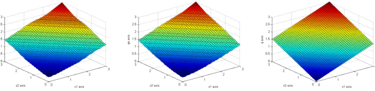
Figure1.:The estimator FN(y|x) versus F (y|x) for N = 100
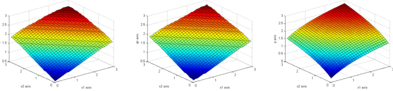
Figure3.:Model 2 :Conditional median surface versus theoretical nonlinear function (right) for N= 200 and N= 500
4. Auxiliary results and proofs
For notational convenience we set
Zi(x, y) = Kd ( x− Xi hK ) H ( y− Yi hH ) − E [ Kd ( x− X1 hK ) H ( y − Y1 hH )] =: Zi.
Then it is clear that we have
F1,N(x, y)− E [F1,N(x, y)] = 1 N hdK N ∑ i=1 Zi.
We recall in the following lemma an exponential inequality stated in Doukhan and Neumann (2007) used in the proof of proposition 1.
LEMMA 1– Under assumptions (H2)(i),(H4) and (H8), there exist constants M0,L1,L2 and µ, λ ≥ 0
such that for all (s1, . . . , su) ∈ Nuand all (t1, . . . , tv) ∈ Nv with 1≤ s1 ≤ . . . ≤ su ≤ t1 ≤ . . . ≤ tv ≤
n, we have (a) cov(∏su i=s1Zi, ∏tv j=t1Zj ) ≤ Cu+vhd Kh 2 d+1 H uv (ρ(t1− su)) d 2d+2 ; (b) ∞ ∑ s=0 (s + 1)k(ρ(s))2d+2d ≤ L1Lk 2(k!) µ,∀k ≥ 0 ; (c) E(|ψi|k ) ≤ (k!)λMk 0,∀k ≥ 0. 4.1. Proof of Lemma 1
To prove this lemma we first recall that Φm : Rm → R is said to be a Lipschitz function if
Lip(Φm) = sup
x̸=y
|Φm(x)− Φm(y)|
where∥z∥1 =|z1| + |z2| + · · · + |zm|. For such a function, the partial Lipschitz constants (see Bulinski and Shashkin 2007, Definition 5.1, p. 88) are
Lipi(Φm) = sup z1,... ,zm,zi′∈R zi̸=zi′ |Φm(z1, . . . , zi−1, zi, zi+1, . . . , zm)− Φm(z1, . . . , zi−1, z ′ i, zi+1, . . . , zm)| |zi− zi′| . [8] So, to state item (a) we set
Φu := su ∏ i=s1 Zi and Φv := tv ∏ j=t1 Zj.
Firstly by using Theorem 5.3 in [BULINSKI and SHASHKIN 2007], the definition in (6) and the fact
that Kd and H are Lipschitz functions we may write
cov (Φu, Φv)≤ su ∑ i=s1 tv ∑ j=t1 Lipi(Φu)Lipj(Φv)ηij.
Next, in view of the definition in (8) and by a simple computation but long enough, we obtain Lipi(Φu) ≤ C hKhH (2∥Kd∥∞) u−1 and Lipi(Φv) ≤ C hKhH (2∥Kd∥∞) v−1 with
C = max{hH∥K∥d∞−1Lip(K), hK∥Kd∥∞Lip(H) }
.
where∥·∥∞stands for the sup norm. Hence by Assumption (H4) and the stationarity we get
cov (Φu, Φv) ≤ C2 (hKhH)2∥K d∥u+v∞ −2 su ∑ i=s1 tv ∑ j=t1 ηij ≤ C (hKhH)2∥K
d∥u+v∞ uvρ(t1− su) =: cov1. [9]
On the other hand, under (H8), a change of variable and (H1)(i) we have
|cov (Zi, Zj)| = |E(ZiZj)| ≤ ∫ Rd ∫ R ∫ Rd ∫ R Kd ( x− u hK ) H ( y− r hH ) Kd ( x− s hK ) H ( y − t hH ) ×fj(u, r, s, t)dudrdsdt) + ∫ Rd ∫ R Kd ( x− u hK ) H ( y− r hH ) f (u, r)dudr
× ∫ Rd ∫ R Kd ( x− s hK ) H ( y − t hH ) f (s, t)dsdt = O(h2dKh2H),
which helps to obtain
|cov (Φu, Φv)| ≤ Cu+vh2dKh
2
H =: cov2. [10]
Then by combining (9) and (10), we get
|cov (Φu, Φv)| ≤ Cu+vhdKh 2 d+1 H uv (ρ(t1− su)) d 2d+2 . [11]
For items (b) and (c), the proofs are similar to those of Proposition 8 in [DOUKHAN and NEUMANN 2007]. It suffices to choose µ = 1, L1 = L2 = (1− e
−τd
2d+2)−1, λ = 0 and use Assumption (H4). Then we
omit them. 2
4.2. Proof of Proposition 1
The proof is based on the following observation : The compacts sets Ω0 and [a, b] can be covered
respectively by a finite number dx,N of balls Bk centred at xk ∈ Rd such that max 1≤k≤dx,N ∥x − xk∥ ≤ ( N−12h d 2+β K )1 β =: ωNd and dy,n intervals Jℓ centred at yℓsatisfying
max
1≤ℓ≤dy,N
|y − yℓ| ≤ hH(nhdK)−
1
2 =: ζn.
Since Ω0and [a, b] are bounded, one can find two positive constants Mx and My such that dx,Nωnd ≤ Mx,
dy,NζN ≤ My and MxMy ≤ C.
Hence we consider the following decomposition sup
x∈Ω0
sup a≤y≤b
|F1,N(x, y) − E[F1,N(x, y)]| ≤ max
1≤k≤dx,N sup x∈Bk sup a≤y≤b |F1,N(x, y)− F1,N(xk, y)| + max 1≤k≤dx,N sup x∈Bk sup a≤y≤b|E[F
1,N(x, y)]− E[F1,N(xk, y)]|
+ max 1≤k≤dx,N max 1≤ℓ≤dy,N sup y∈Jℓ |F1,N(xk, yℓ)− F1,N(xk, y)| + max 1≤k≤dx,N max 1≤ℓ≤dy,N sup y∈Jℓ
|E[F1,N(xk, yℓ)]− E[F1,N(xk, y)]|
+ max 1≤k≤dx,N max 1≤ℓ≤dy,N |F1,N(xk, yℓ)− E[F1,N(xk, yℓ)]| = I1N +I ′ 1N +I2N +I ′ 2N +I3N. [12]
Under assumptions (H1)(i) we have
|F1,N(x, y)− F1,N(xk, y)| ≤ C∥x − x k∥ β hβK 1 N hd K N ∑ i=1 H ( y − Yi hH )
≤ C(ωNd)β
hd+βK
= O((N hdK)−1/2
)
. [13]
Similar arguments as above lead to the same bound forI1N′ .
Under (H2), and according to Markov inequality and the Dominated Convergence Theorem we obtain
the same upper-bound forI2N. We have
|F1,n(xk, yℓ)− F1,N(xk, y)| ≤ C|y − y ℓ| hH 1 N hdK N ∑ i=1 Kd ( xk − Xi hK ) ≤ CζN hH 1 N hdK N ∑ i=1 Kd ( xk − Xi hK ) ≤ C ζN hH) vN(x) = O((N hdK)−1/2 ) . [14]
The termI2N′ is upper-bounded similarly asI2N. We now turn to the term I3n we use Theorem 1 of
[DOUKHAN and NEUMANN 2007]. For this, consider the centered random functions Zi(xk, yℓ); i =
1, . . . , n satisfying the items in Lemma 1. Then for any ε > 0 we have P ( N ∑ i=1 Zi(xk, yℓ)≥ ε ) ≤ exp ( − ε2/2 AN + B 1/(µ+λ+2) N ε(2µ+2λ+3)/(µ+λ+2) ) , [15]
where AN and BN can be chosen such that
AN ≤ σ2N with σ 2 N := var ( N ∑ i=1 Zi(xk, yℓ) ) and BN = 2CL2 24+µ+λCN hdKh 2 d+1 H L1 AN ∨ 1 . For this purpose, we first evaluate σN2 .
σN2 = var ( N ∑ i=1 Zi(xk, yℓ) ) = var ( N hdKF˜1,n(xk, yℓ) ) = N var ( Kd ( xk − X1 hK ) H ( yℓ− Y1 hH )) + N ∑ i=1 N ∑ j=1 cov ( Kd ( xk− Xi hK ) H ( yℓ− Yi hH ) , Kd ( xk− Xj hK ) H ( yℓ− Yj hH )) =: V + S .
On the one hand we have
V = N { E [ Kd2 ( xk− X1 hK ) H2 ( yℓ− Y1 hH )] − E2 [ Kd ( xk − X1 hK ) H ( yℓ− Y1 hH )]}
=: N{V1− V2} .
By a change of variable, a Taylor expansion, assumptions (H1)(i) (ii),(H2)(i) and (H7) we get
V1 = E [ Kd2 ( xk − X1 hK ) H2 ( yℓ− Y1 hH )] ≤ ∫ Rd Kd2 ( xk − u hK ) ∫ R f (u, s)ds du, car H(·) ≤ Chd K ∫ Rd Kd2(z)v(xk − zhK)dz = O(hdK).
ForV2we work as forV1. Under assumptions (H1)(i) (ii),(H2)(i),(H7), a change of variable and a Taylor
expansion, we get V2 = E2 [ Kd ( xk − X1 hK ) H ( yℓ− Y1 hH )] = O(h2dK), ThusV = O(NhdK).
Now to deal withS , let us define B1 ={(i, j); 1 ≤ |i−j| ≤ wN} and B2 ={(i, j); wN+ 1≤ |i−j| ≤
N − 1}, where wN = o(N ). Then
S = N ∑ i=1 ∑ j∈B1 cov ( Kd ( xk − Xi hK ) H ( yℓ− Yi hH ) , Kd ( xk− Xj hK ) H ( yℓ− Yj hH )) + N ∑ i=1 ∑ j∈B2 cov ( Kd ( xk − Xi hK ) H ( yℓ− Yi hH ) , Kd ( xk− Xj hK ) H ( yℓ− Yj hH )) =: S1+S2. From (10) we get S1 = O ( N wNh2dKh 2 H ) .
Then under Assumption (M) and taking u = v = 1 in (11), we can write
S2 ≤ N ∑ i=1 ∑ j∈B2 C2hdKh 2 d+1 H (ρ(|i − j|)) d 2d+2 ≤ CNhd Kh 2 d+1 H ∑ l∈B2 e−τ2d+2|i−j|d ≤ CNhd Kh 2 d+1 H N ∫ wN e−2d+2τ dξ dξ
= O ( N hdKh 2 d+1 H e− τ dwN 2d+2 ) .
So, under Assumption (B)(i)(ii) and choosing wN = O
( hν1−d K h ν2−1 H ) with 0 < ν1 < d and 0 < ν2 < 1, the terms S1 and S2 become of order o(N hdKhH) and o(N hdKh
2 d+1 H ), respectively. Hence, S = o(Nhd Kh 2 d+1
H ) and σ2N = O(N hdK) and therefore we can take AN = O(N hdK). In addition, by
choosing µ, λ, L1 and L2 as before in proving Lemma 1, we get BN = O(1). Consequently (15)
be-comes P ( N ∑ i=1 Zi(xk, yℓ)≥ ε ) ≤ exp ( − ε2/2 CN hdK + ε53 ) . [16] Furthermore, if we choose ε = ε0 √ log N N hd K
; ε0 > 0, then from (16) we have
P (I3N ≥ ε) = P ( max 1≤k≤dx,N max 1≤ℓ≤dy,N N ∑ i=1 Zi(xk, yℓ) ≥ εN hdK ) ≤ 2dx,Ndy,N exp ( − (εN hdK) 2/2 CN hdK + (εN hdK)53 ) ≤ C(ωd N)−1ζN−1exp − (ε 2 0log N )/2 C + ε 5 3 0 ( log5N N hd K )1/6 ≤ C(N−12h d 2+β K )−1 β ( (N hK)− 1 2hH )−1 N−Cε20 = ( N hd(1K −β)+2β )− 1 2β (N hH)−1O ( N−Cε20+β1+ 3 2 ) . [17]
Then, for an appropriate choice of ε0 and Assumption(H1) (i) (ii), the term in (17) becomes an O(N−θ)
with θ > 1. So, we obtain
P ( I3N ≥ ε0 √ log N N hdK ) = O(n−θ). [18]
Hence, according to (12),(13),(14) and (18), if we set ε1 = 5ε0, it follows that
∑ n≥1 P ( sup x∈Ω0 sup a≤y≤b|F 1,N(x, y)− E[F1,N(x, y)]| ≥ ε1 √ log N N hd K ) ≤ ∑ N≥1 P ( I3N ≥ ε0 √ log N N hd K ) <∞.
Thus by the Borel-Cantelli lemma, we conclude that
sup x∈Ω0 sup a≤y≤b |F1,N(x, y)− E [F1,N(x, y)]| = O (√ log N N hd K ) P-a.s., as N → ∞.
LEMMA 2– Under assumptions (H2),(H3) and (H7) we have sup x∈Ω0 sup a≤y≤b|E [F 1,N(x, y)]− F1(x, y)| = O(h2K + h 2 H). 4.3. Proof of Lemma 2
The proof is based on integration by parts, a change of variable and a Taylor expansion, indeed we have E [F1,n(x, y)]− F1(x, y) = E [ 1 nhdK N ∑ i=1 Kd ( x− Xi hK ) H ( y− Yi hH )] − F1(x, y) = 1 hdK ∫ Rd Kd ( x− r hK ) ∫ R H(1)(s) F1(r, y− shH)ds dr − F1(x, y) = ∫ Rd ∫ R
Kd(u) H(1)(s) (F1(x− uhK, y− shH)− F1(x, y)) duds.
Then under assumptions (H2),(H3) and (H7) we get sup
x∈Ω0
sup a≤y≤b|E [F
1,n(x, y)]− F1(x, y)| = O(h2K + h2H).
The proof of Lemma 2 is finished. 2
LEMMA 3– Under assumptions (H1)(i),(H2)and (H4)−(H6) we have
sup x∈Ω0 |vN(x)− v(x)| = O (√ log N N hd K + h2K ) P-a.s., as N → ∞. 4.4. Proof of Lemma 3 We have sup x∈Ω0 |vN(x)− v(x)| ≤ sup x∈Ω0 |vN(x)− E[vN(x)]| + sup x∈Ω0 |E[vN(x)]− v(x)|
suggests to treat the first term in the right-hand side by following the same steps and similar arguments used in proving Proposition 1. Hence we get
sup x∈Ω0 |vN(x)− E[vN(x)]| = O (√ log N N hdK ) P-p.s., as N → ∞.
Furthermore, under assumptions (H1)(i),(H2)and (H5) and using a Taylor expansion, we get sup
x∈Ω0
|E[vN(x)]− v(x)| = O(h2K).
4.5. Proof of Theorem 1
The proof is based on the following decomposition.
sup x∈Ω0 sup a≤y≤b|F N(y|x) − F (y|x)| ≤ 1 γ− sup x∈Ω0 |vN(x)− v(x)| { sup x∈Ω0 sup a≤y≤b|F 1,N(x, y)− E[F1,N(x, y)]| + sup x∈Ω0 sup a≤y≤b |E[F1,N(x, y)]− F1,N(x, y)| +γ−1 sup x∈Ω0 sup a≤y≤b F1(x, y)× sup x∈Ω0 |vN(x)− v(x)| }
Then by using Proposition 1, Lemma 2 and Lemma 3 we get the result.
4.6. Proof of Corollary 1
A Taylor series expansion of F (qp,N(·)|·) around qp(·) gives
F (qp,N(x)|x) − F (qp(x)|x) = (qp,N(x)− qp(x)) f (
qp,N∗ (x)|x),
where qp,N∗ (x) lies between qp(x) and qp,N(x). Hence, by standard arguments we can write
|F (qp,N(x)|x) − F (qp(x)|x)| ≤ 2 sup a≤y≤b|F
N(y|x) − F (y|x)| ,
which implies that sup x∈Ω0 |qp,N(x)− qp(x)| f ( qp,N∗ (x)|x)≤ 2 sup x∈Ω0 sup a≤y≤b |FN(y|x) − F (y|x)| .
Thus, by Theorem 1 and because f (qp(·)|·) is uniformly lower-bounded away from zero, we assert that
sup x∈Ω0 |qp,N(x)− qp(x)| = O (√ log N N hd K + h2K + h2H ) P-p.s., as n → ∞.
This ends the proof of Corollary 1. 2
Bibliographie
BULINSKI A., SHASHKINA., Limit theorems for associated random fields and related systems. Singapore World Scien-tific, 2007.
DOUKHANP., NEUMANNM., Probability and moment inequalities for sums of weakly dependent random variables, with applications. Stochastic Processes and their Applications 117 (2007) : 878-903.
CHAUDHURI P., DOKSUMK., SAMAROV A., On average derivative quantile regression. Ann. Statist. 25 (1997) : 715– 744.
ESARYJ., PROSCHANF., WALKUPD., Association of random variables with applications. Ann. Math. Stat. 38 (1967) : 1466-1476.
HONDA T., Nonparametric estimation of a conditional quantile for strong mixing processes. Ann. Inst. Statist. Math. 52 (2000) :459–470.
MEHRAK.L., RAOM.S., UPADRASTAS.P., A smooth conditional quantile estimator and related applications of condi-tional empirical processes. J. Multivariate Anal. 37 (1991) :151-179
OLIVEIRA P.E., Asymptotics for Associated Random Variables. Springer Verlag, 2012.
PRAKASA RAO B.L.S., Associated Sequences, Demimartingales and Nonparametric Inference. Probability and its Ap-plications, Springer Basel AG, 2012
XIANG X., A kernel estimator of a conditional quantile, J. Multivariate Anal. 59 (1996) : 206-216. YU K., JONESM.C., Local linear quantile regression. J. Am. Stat. Assoc. 93 (1998) : 228-238