Complex Job Shop Scheduling:
A General Model and Method
Thesis
presented to the Faculty of Economics and Social Sciences at the University of Fribourg, Switzerland,
in fulfillment of the requirements for the degree of Doctor of Economics and Social Sciences by
Reinhard B¨
urgy
from Gurmels (FR)
Accepted by the Faculty of Economics and Social Sciences on February 24th, 2014 at the proposal of
Prof. Dr. Heinz Gr¨oflin (first advisor) Prof. Dr. Marino Widmer (second advisor) Prof. Dr. Dominique de Werra (third advisor)
The Faculty of Economics and Social Sciences at the University of Fribourg neither approves nor disapproves the opinions expressed in a doctoral thesis. They are to be considered those of the author. (Decision of the Faculty Council of January 23rd, 1990).
To my wife Emmi and
our precious daughter Saimi
This thesis would not have been possible without the countless contributions of many people, to whom I wish to express my sincerest gratitude. In particular, I am greatly indebted to:
My thesis supervisor Prof. Heinz Gr¨oflin, for the opportunity to work in the area of Operations Research and to discover the fascinating world of scheduling. This thesis would not have been possible without his enthusiastic, acute, illuminating, patient support and guidance. His integrity and insights to education and science will always be a source of inspiration for me.
Prof. Marino Widmer and Prof. Dominique de Werra, for kindly accepting to be reviewers of my thesis.
Tony H¨urlimann, not only for providing his excellent mathematical modeling language LPL, but also for many insightful discussions throughout the last years.
Prof. Pius H¨attenschwiler and his former collaborators Matthias Buchs and Michael Hayoz for the precious time I could spend with them as an undergraduate assistant. Their encouraging guidance let me gain priceless experience and knowledge.
Ivo Bl¨ochliger, Christian Eichenberger, Andreas Humm, Stephan Krenn, Antoine Legrain, Marc Pouly and Marc Uldry for their friendly support.
My parents Bernadette and Rudolf and my sister Stefanie, for their love and unfal-tering support and encouragement. Their warm generosity and precious values will always be an example to me.
My wife Emmi, for being with me. With all my heart, I thank you for your presence, patience, warmth and love.
Scheduling is a pervasive task in planning processes in industry and services, and has become a dedicated research field in Operations Research over the years. A core of standard scheduling problems, models and methods has been developed, and substantial progress has been made in the ability to tackle these difficult combinatorial optimization problems.
Nevertheless, applying this body of knowledge is often hindered in practice by the presence of features that are not captured by the standard models, and practical scheduling problems are often treated ad-hoc in their application context. This “gap” between theory and practice has been widely acknowledged also in scheduling prob-lems of the so-called job shop type. This thesis aims at contributing to narrow this gap.
A general model, the Complex Job Shop (CJS) model, is proposed that includes a variety of features from practice, including no (or limited number of) buffers, routing flexibility, transfer and transport operations, setup times, release times and due dates. The CJS is then formulated as a combinatorial problem in a general disjunctive graph based on a job template and an event-node representation.
A general solution approach is developed that is applicable to a large class of CJS problems. The method is a local search heuristic characterized by a job insertion based neighborhood and named JIBLS (Job Insertion Based Local Search). A key feature of the method is the ability to consistently and efficiently generate feasible neighbor solutions, typically by moving a critical operation (keeping or changing the assigned machine) together with other operations whose moves are “implied”. For this purpose, the framework of job insertion with local flexibility, introduced in [45] and the insertion theory developed by Gr¨oflin and Klinkert [42] are used. The meta-heuristic component of the JIBLS is of the tabu search type.
The CJS model and the JIBLS method are validated by applying them to a selection of complex job shop problems. Some of the selected problems have been studied by other authors and benchmarks are available, while the others are new. Among the first are the Flexible Job Shop with Setup Times (FJSS), the Job Shop with
VIII
Transportation (JS-T) and the Blocking Job Shop (BJS), and among the second are the Flexible Blocking Job Shop with Transfer and Setup Times (FBJSS), the Blocking Job Shop with Transportation (BJS-T) and the Blocking Job Shop with Rail-Bound Transportation (BJS-RT). Of particular interest is the BJS-RT, where the transportation robots interfere with each other, which is, to our knowledge, the first generic job shop scheduling problem of this type.
For the problems with available benchmarks it is shown that the JIBLS is compet-itive with the best (often problem-tailored) methods of the literature. Moreover, the JIBLS appears to perform well also in the new problems and provides first benchmarks for future research on these problems.
Altogether, the results obtained provide evidence for the broad applicability of the CJS model and the JIBLS, and for the good performance of the JIBLS compared to the state of the art.
1. Introduction 1
1.1. Scheduling . . . 1
1.2. Some Scheduling Activities in Practice . . . 2
1.2.1. Scheduling in Production Planning and Control . . . 2
1.2.2. Project Scheduling . . . 5
1.2.3. Workforce Scheduling . . . 5
1.2.4. Scheduling Reservations and Appointments . . . 5
1.2.5. Pricing and Revenue Management . . . 6
1.3. Some Generic Scheduling Problems . . . 6
1.3.1. The Resource-Constrained Project Scheduling Problem . . . . 6
1.3.2. The Machine Scheduling Problem . . . 7
1.3.3. The Classical Job Shop Scheduling Problem . . . 8
1.4. Extensions of the Classical Job Shop . . . 9
1.4.1. Setup Times . . . 9
1.4.2. Release Times and Due Dates . . . 10
1.4.3. Limited Number of Buffers and Transfer Times . . . 11
1.4.4. Time Lags and No-Wait . . . 12
1.4.5. Routing Flexibility . . . 13
1.4.6. Transports . . . 14
1.5. Overview of the Thesis . . . 14
I.
Complex Job Shop Scheduling
19
2. Modeling Complex Job Shops 21 2.1. Introduction . . . 212.2. Some Formulations of the Classical Job Shop . . . 22
2.2.1. A Disjunctive Programming Formulation . . . 22
X Contents
2.2.3. A Disjunctive Graph Formulation . . . 23
2.2.4. An Example . . . 23
2.3. A Generalized Scheduling Model . . . 24
2.3.1. A Disjunctive Programming Formulation . . . 25
2.3.2. A Disjunctive Graph Formulation . . . 25
2.4. A Complex Job Shop Model (CJS) . . . 27
2.4.1. Building Blocks of the CJS Model and a Problem Statement . 27 2.4.2. Notation and Data . . . 28
2.4.3. A Disjunctive Graph Formulation . . . 30
2.4.4. An Example . . . 32
2.4.5. Modeling Features in the CJS Model . . . 34
3. A Solution Approach 37 3.1. Introduction . . . 37
3.2. The Local Search Principle . . . 38
3.2.1. The Local Search Principle in the Example . . . 38
3.2.2. The Job Insertion Graph with Local Flexibility . . . 41
3.3. Structural Properties of Job Insertion . . . 42
3.3.1. The Short Cycle Property . . . 42
3.3.2. The Conflict Graph and the Fundamental Theorem . . . 47
3.3.3. A Closure Operator . . . 48
3.4. Neighbor Generation . . . 53
3.4.1. Non-Flexible Neighbors . . . 53
3.4.2. Flexible Neighbors . . . 54
3.4.3. A Neighborhood . . . 55
3.5. The Job Insertion Based Local Search (JIBLS) . . . 56
3.5.1. From Local Search to Tabu Search . . . 56
3.5.2. The Tabu Search in the JIBLS . . . 57
II. The JIBLS in a Selection of CJS Problems
61
4. The Flexible Job Shop with Setup Times (FJSS) 63 4.1. Introduction . . . 634.2. A Literature Review . . . 63
4.3. A Problem Formulation . . . 65
4.4. The FJSS as an Instance of the CJS Model . . . 65
4.5. A Compact Disjunctive Graph Formulation . . . 66
4.6. Specifics of the Solution Approach . . . 67
4.6.1. The Closure Operator . . . 67
4.6.2. Feasible Neighbors by Single Reversals . . . 68
4.6.3. Critical Blocks . . . 70
4.7. Computational Results . . . 71
5. The Flexible Blocking Job Shop with Transfer and Setup Times (FBJSS) 79 5.1. Introduction . . . 79
5.2. A Literature Review . . . 80
5.3. A Problem Formulation . . . 80
5.4. The FBJSS as an Instance of the CJS Model . . . 81
5.5. Computational Results . . . 81
5.6. From No-Buffers to Limited Buffer Capacity . . . 89
6. Transportation in Complex Job Shops 95 6.1. Introduction . . . 95
6.2. A Literature Review . . . 96
6.3. The Job Shop with Transportation (JS-T) . . . 98
6.3.1. A Problem Formulation . . . 98
6.3.2. Computational Results . . . 99
6.4. The Blocking Job Shop with Transportation (BJS-T) . . . 104
6.4.1. A Problem Formulation . . . 104
6.4.2. Computational Results . . . 104
7. The Blocking Job Shop with Rail-Bound Transportation (BJS-RT) 109 7.1. Introduction . . . 109
7.2. Notation and Data . . . 110
7.3. A First Problem Formulation . . . 111
7.3.1. The Flexible Blocking Job Shop Relaxation . . . 111
7.3.2. Schedules with Trajectories . . . 112
7.4. A Compact Problem Formulation . . . 113
7.4.1. The Feasible Trajectory Problem . . . 114
7.4.2. Projection onto the Space of Schedules . . . 118
7.5. The BJS-RT as an Instance of the CJS Model . . . 119
7.6. Computational Results . . . 120
7.7. Finding Feasible Trajectories . . . 124
7.7.1. Trajectories with Variable Speeds . . . 124
7.7.2. Stop-and-Go Trajectories . . . 130
8. Conclusion 137
BJS Blocking Job Shop
BJSS Blocking Job Shop with Transfer and Setup Times BJS-RT Blocking Job Shop with Rail-Bound Transportation BJS-T Blocking Job Shop with Transportation
CJS Complex Job Shop
JS Job Shop
JSS Job Shop with Setup Times JS-T Job Shop with Transportation FBJS Flexible Blocking Job Shop
FBJSS Flexible Blocking Job Shop with Transfer and Setup Times FJS Flexible Job Shop
FJSS Flexible Job Shop with Setup Times FNWJS Flexible No-Wait Job Shop
FNWJSS Flexible No-Wait Job Shop with Setup Times JIBLS Job Insertion Based Local Search
MS Machine Scheduling
MIP Mixed Integer Linear Programming MPS Master Production Schedule MRP Material Requirement Planning MRP II Manufacturing Resource Planning II NWJS No-Wait Job Shop
NWJSS No-Wait Job Shop with Setup Times NWJS-T No-Wait Job Shop with Transportation RCPS Resource-Constrained Project Scheduling SCP Short Cycle Property
INTRODUCTION
The topic of the thesis, complex job shop scheduling, is introduced in this chapter as follows. Section 1.1 describes the concept of scheduling. Section 1.2 presents common scheduling activities in practice. Some generic scheduling problems are specified in Section 1.3, starting with the resource-constrained project scheduling problem, and specializing it to the machine scheduling problem and the classical job shop scheduling problem, which is the basic version of the problems treated in this thesis. A variety of complexifying features that arise in practice and are not taken into account in the classical job shop are discussed in Section 1.4. Finally, Section 1.5 gives an overview of the thesis.
This chapter is mainly based on the operations management textbooks of Jacobs et al. [24] and Stevenson [108], and on the scheduling textbooks of Baker and Trietsch [7], Blazewicz et al. [11], Brucker and Knust [17] and Pinedo [95, 96].
1.1. Scheduling
Schedules are part of our professional and personal life. They answer the question of knowing when specific activities should happen and which resources are used. We mention just a few examples: bus schedules, also called bus timetables, contain ar-rival and departure times for each bus and bus stop; school timetables consist of the schedule for each class indicating lessons, teachers, rooms and time; project sched-ules comprise start and finish times of their activities; tournament schedsched-ules indicate which teams play against each other at which time and location; production sched-ules provide information on the orders stating when they should be executed on which equipment.
The term scheduling refers to the process of generating a schedule, which is com-monly described as follows. The objects that are scheduled are called activities. Activities are somehow interrelated by so-called technological restrictions, e.g. some
2 1.2. SOME SCHEDULING ACTIVITIES IN PRACTICE
activities must be finished before others can start. For its execution each activity needs some resources which may be chosen from several alternative resources. The resources typically have limited capacity. A schedule consists of an allocation of re-sources and a starting time for each activity so that the capacity and technological restrictions are satisfied. The goal in scheduling is to find an optimal schedule, i.e. a schedule that optimizes some objective. The objective is typically related to time, for example minimizing the makespan, i.e. the overall time needed to execute all activities, minimizing the throughput times or minimizing the setup times.
Scheduling is performed in every organization. It is the final planning step before the actual execution of the activities. Hence, it links the planning and execution phases. While a short time horizon is often considered, detailed schedules are needed long before their actual execution in some industries (e.g. in the pharmaceutical sector). As future is uncertain, schedules may have to be revised quite frequently, for example due to changes in the shop floor or new order arrivals. Typically, scheduling is done over a rolling time horizon, the earlier part of the schedule being frozen and the remaining part being rescheduled.
Schedules are sometimes generated in an ad-hoc, rather informal way, using e.g. rules of thumb and blackboards. However, a systematic approach is needed for many scheduling problems in order to be able to cope with its complexity. Models and information systems may support the decision makers, allowing to find good or opti-mal schedules. Two types of models can be distinguished: descriptive models offering what if analyses and optimization models attempting to answer what’s best. The models may be embedded in information systems that range from simple spread-sheets of restricted functionality to elaborate decision support systems that offer var-ious (graphical) representations of the models and solutions, interaction of the users and collaborative decision making. Which level of support is needed mainly depends on the difficulty and importance of the scheduling problem.
1.2. Some Scheduling Activities in Practice
In this section, some scheduling activities commonly arising in practice are described.
1.2.1. Scheduling in Production Planning and Control
A typical scheduling task in manufacturing companies with a make to stock strategy concerns production planning and control, for instance in a Manufacturing Resource Planning II (MRP II) approach, which is depicted in Figure 1.1 and explained here briefly.
MRP II is hierarchically structured. At the top level, it comprises the following three phases: i) master planning, ii) detailed planning, and iii) short term planning and control.
Master planning considers a long term planning horizon (i.e. typically up to a year) and consists of sales and operations planning and master scheduling. Sales and operations planning establishes a sales plan and a production plan. On an aggregated
Sales & opera-tions planning
Resource require-ment planning
Master scheduling Rough-cut ca-pacity planning Material require-ment planning Capacity require-ment planning Scheduling
Shop floor control
Aggregated production plan
Master production schedule
Planned orders Released orders Long te rm: master planning Medium term: detailed planning Short term: short term plan-ning and con trol
Figure 1.1.: Production planning and control phases according to MRP II, adapted from Sch¨onsleben [102]. Tasks are depicted in rounded boxes. The lines indicate the exchange of information between the tasks.
4 1.2. SOME SCHEDULING ACTIVITIES IN PRACTICE
level they describe the expected demands and the quantities that should be produced (or bought) for each product family and time unit. Resource requirements are also considered when establishing the production plan, looking at aggregated resources and focusing on critical resources. Based on the aggregated production plan, inventory stock levels and stock policies, the Master Production Schedule (MPS) is established in the master scheduling, stating the needed quantity for each end product and time period of the planning horizon. Feasibility of the MPS is considered in rough-cut capacity planning. If capacities are not sufficient, the MPS may be revised.
The detailed planning phase links the master planning with short term planning and control. It considers a medium term planning horizon (i.e. typically some months) and consists of the Material Requirement Planning (MRP) and the capacity require-ment planning. Based on the MPS, bills of material, inventory stock levels and production lead time estimations, the MRP determines the needed quantity to fulfill the MPS for each component (raw material, parts, subassemblies) and time period. The outputs of this phase are planned (production and purchase) orders. Capacity requirement planning checks if enough capacity is present to produce the orders as planned. If capacities are not sufficient, the planning may be revised or capacities may be adjusted.
The final planning phase consists of scheduling the planned orders for the next days and weeks. A fine-grained schedule is established, determining the execution time and the assigned resources for each processing step of the planned orders. The schedule must be feasible; particularly, it must satisfy the capacity restrictions. The capacities of the resources are considered on a fine-grained level, e.g. a resource can execute at most one order at any time. To guarantee feasibility, the characteristic features of the production system must be considered in scheduling.
The outputs of the scheduling phase, called released orders, are then used in the shop floor to control the actual production.
Note that feedbacks from a phase to previous phases are common as indicated by the dashed lines in Figure 1.1. For example, unexpected events in the shop floor, such as machine failures or quality problems, may force to reschedule some orders. Minor problems may be dealt with at the control level. Whenever encountering major problems, the control level feeds back the inputs to the scheduling and a new schedule is generated.
At first glance, the decisions in scheduling appear to have a limited scope com-pared to, for example, system design decisions and longer term planning decisions. This view does not reflect the high impact of scheduling in production planning and control. In fact, good scheduling may lead to cost reductions and a greater flexibility in previous planning phases, such as working with less machines or accepting more customer orders, and bad scheduling may lead to due date violations and idle times so that costly actions are needed, such as the purchase of new machines or over-time work. Furthermore, scheduling may also reveal problems in the system design such as bottlenecks and problems in the longer term planning such as too optimistic production lead time and due date estimations.
Several trends, including mass customization and the adoption of complex auto-mated production systems, suggest that the importance and difficulty of scheduling problems in production planning will increase in the future.
1.2.2. Project Scheduling
Projects are unique, one-time operations set up to achieve some objectives given a limited amount of resources such as money, time, machines and workers.
Projects arise in every organization. Typical examples are the development of a product, the construction of a factory and the development and integration of software.
The management of a project consists in planning, controlling and monitoring the project so that quality, time, cost and other project requirements are met. Important aspects in project planning include breaking down the project into smaller compo-nents, such as sub-projects, tasks, work packages and activities, and establishing a schedule of the project.
Scheduling a project consists in assigning starting times to all activities and assign-ing resources to the activities so that a set of goals are achieved and all constraints are satisfied. The goals and constraints are typically related to time, resources or costs. For example, the project duration may be minimized, the activities are interrelated, e.g. by precedence constraints, and can have deadlines, a smooth resource utilization may be sought, and total costs may be minimized.
1.2.3. Workforce Scheduling
In many organizations, a work plan for the work force must be established, determin-ing for all workers when they are workdetermin-ing and what they are workdetermin-ing on. The goal may be to minimize costs.
The workers have to be scheduled so that the needed demand is met, e.g. enough workers are assigned to execute the production plan or to serve the customers. A variety of specific working constraints make the problem different from other schedul-ing problems. A machine may be used durschedul-ing the whole day and seven days a week. Workers, however, have specific working restrictions, such as a work time limit per day and week, and regulations on breaks and free days.
1.2.4. Scheduling Reservations and Appointments
In the service industry, services are sometimes requested and reserved prior to their consumption. Besides decisions on the timing and the allocation of resources, the reservation process allows controlling the acceptance of the requests.
Two main types of scheduling problems are distinguished. The first type, called reservation scheduling, occurs if the customers have no or almost no flexibility in time, i.e. the time of the service consumption is fixed. The main decision is whether to accept or deny a service request, and the objective is often to maximize resource
6 1.3. SOME GENERIC SCHEDULING PROBLEMS
utilization. Such types of decisions are quite common in many sectors including the transportation industry (car rentals, air and train transportation) and hotels.
The second type, called appointment scheduling, consists of scheduling problems where the customers have more flexibility in time. The main decision is the timing of the service. Appointment scheduling problems are common in practice, e.g. for business meetings, appointments at the doctor’s office and at the hairdresser.
In both types of problems, cancellations and customers that do not show up or show up late must be taken into account, increasing the complexity of the problem.
1.2.5. Pricing and Revenue Management
In an integrated scheduling approach, service requests are not just accepted or denied, but variable pricing is established to control demand. The prices are typically set by analyzing specifics of the request, left capacities and demand forecasts. This so-called tactical pricing leads to different prices for the same or similar services. An increase of the profit, better resource utilization and the gain of new customers are some of the goals of tactical pricing.
While not being a standard technique in manufacturing, tactical pricing is com-monly used in the service industry. Well-known examples are the pricing of flight tickets and hotel accommodations. For example, a flight request of a customer three days before departure is likely to be priced higher than the same request made three months earlier.
When services are requested prior to consumption, pricing and reservation schedul-ing may be combined, formschedul-ing so-called revenue management problems. These prob-lems are well-known in the airline and hotel industries.
Tactical pricing is also present in sectors with no service reservation such as in supermarkets and coffee shops. The prices may depend on the channels (e.g. are cheaper through the internet), the time of consumption (e.g. the coffee is cheaper in the morning), or product variations are created (e.g. budget or fine food lines).
1.3. Some Generic Scheduling Problems
As described in the previous section, scheduling is a pervasive activity in practice. In scheduling theory, a core of generic scheduling problems, models and methods has been developed for solving these problems. In this section we introduce some generic scheduling problems, starting with the resource-constrained project scheduling problem, and specializing it to the machine scheduling problem and the classical job shop scheduling problem.
1.3.1. The Resource-Constrained Project Scheduling Problem
A general scheduling problem is the Resource-Constrained Project Scheduling (RCPS) problem, which can be specified as follows. Given is a set of activities I and a set of resources R. Each resource r ∈ R is available at any time in amount Br. Each
activity i ∈ I requires an amount briof each resource r ∈ R during its non-preemptive execution of duration di ≥ 0. Some activities must be executed before others can start. These so-called precedence constraints are given by a set P of pairs of activities (i, j), i, j ∈ I, where i has to be completed before j can start. The objective is to specify a starting time αi for each activity i ∈ I so that the described constraints are satisfied and the project duration is minimized.
Introduce a fictive start activity σ and a fictive end activity τ and let I+= I ∪{σ, τ }. Activities σ and τ are of duration 0 and must occur before, respectively after all activities of I. Then, the RCPS problem can be formulated as follows:
minimize ατ (1.1)
subject to:
αi− ασ ≥ 0 for all i ∈ I, (1.2) ατ− αi≥ di for all i ∈ I, (1.3) αj− αi≥ di for all (i, j) ∈ P, (1.4) For all r ∈ R :
X i∈I:αi≤t≤αi+di
bri≤ Brat any time t, (1.5)
ασ = 0. (1.6)
Any feasible solution α ∈ RI+
is called a schedule. The starting time ασ is set to 0 (1.6) and ατ reflects the project duration, which is minimized (1.1). Constraints (1.2), (1.3) and (1.4) ensure that all activities are executed in the right order between start and end. The capacity constraints (1.5) ensure that at any time, the activities in execution require no more of resource r than available.
Clearly, the capacity constraints (1.5) are not tractable in this form. Other, more tractable versions exist (see e.g. Brucker and Knust [17]). However, regardless of the formulation, the RCPS problem is a difficult problem to solve.
1.3.2. The Machine Scheduling Problem
An important special type of RCPS is the Machine Scheduling (MS) problem, where each resource r ∈ R has capacity Br= 1 and each activity has a requirement bri= 0 or bri = 1 for each r ∈ R. Consequently, a resource is either free or occupied by an activity, and for any two distinct activities i, j needing a same resource r, i must precede j or vice versa.
Let Q be a set containing all unordered pairs {i, j} of distinct operations i, j ∈ I needing a same resource, i.e. for some r ∈ R, bri = brj = 1. Then, the capacity constraints (1.5) can be rewritten in the substantially simpler form of disjunctive constraints:
8 1.3. SOME GENERIC SCHEDULING PROBLEMS
and the MS problem can be formulated as a disjunctive program by (1.1)-(1.4), (1.6) and (1.7).
As early studies of the MS problem were in an industrial context, the resources are called machines and the activities are operations. These terms have become standard and will be used in this thesis, although a resource might not be a machine but any other processor, such as a buffer or a mobile device. In line with common notation, we use letter M for the set of machines (instead of letter R).
1.3.3. The Classical Job Shop Scheduling Problem
An important special type of MS is the classical Job Shop (JS) problem, which has the following features:
• Any operation i ∈ I needs exactly one machine, say mi∈ M , for its execution. Consequently, the set Q contains all unordered pairs {i, j} with i, j ∈ I, i 6= j and mi= mj.
• The set I of operations is partitioned into a set of jobs J : A job J ∈ J is a set of operations {i : i ∈ J } and each operation i ∈ I is in exactly one job J ∈ J . • The set of operations of each job J ∈ J is ordered in a sequence, i.e. {i : i ∈ J }
is sometimes referred to as the ordered set {J1, J2, . . . , J|J |}, Jr denoting the r-th operation of job J .
• The operations of a job J ∈ J have to be processed in sequence, i.e. Jrmust be finished before Jr+1starts, r = 1, . . . , |J | − 1. No other precedence constraints exist. Consequently, the set P consists of all pairs (Jr, Jr+1), 1 ≤ r < |J |, J ∈ J . Denote by Ifirstand Ilastthe subsets of operations that are first and last operations of jobs, respectively, and call two operations i, j of a job J to be consecutive if i = Jr and j = Jr+1for some r, 1 ≤ r < |J |. Then, constraints (1.2), (1.3) and (1.4) can be rewritten as (1.9), (1.10) and (1.11), respectively, giving the following formulation of the JS as a disjunctive program:
minimize ατ (1.8)
subject to:
αi− ασ ≥ 0 for all i ∈ Ifirst, (1.9)
ατ− αi ≥ di for all i ∈ Ilast, (1.10) αj− αi ≥ di for all i, j ∈ I consecutive in some job J, (1.11) αj− αi ≥ di or αi− αj≥ dj for all {i, j} ∈ Q, (1.12)
ασ = 0. (1.13)
A small job shop example is introduced in Figure 1.2. It consists of three machines and three jobs, each visiting all machines exactly once. The figure depicts a solution with makespan 14 in a Gantt chart. The bars represent the operations that are indicated by the attributed numbers, e.g. the bar with number 2.3 refers to the third operation of job 2. The routing of the jobs as well as the processing durations can be read directly in the chart.
4 8 12 16 20 24 t m1 m2 m3 1.1 3.2 2.3 2.1 1.2 3.3 3.1 2.2 1.3
Figure 1.2.: A solution of a small job shop example.
The term “job shop” refers to a manufacturing process type that is generally used when a rather low volume of high-variety products is produced. The high flexibility established by general-purpose machines is a main characteristic of the job shop. The flexibility makes it possible to treat jobs that differ considerably in processing requirements including processing steps, processing times and setups.
Job shop scheduling problems or variations of it arise in industries adopting job shop or similar production systems such as the chemical and pharmaceutical sectors [100], the semiconductor industry [78] and the electroplating sector [68]. Job shop scheduling problems are also present in the service sector such as in transportation systems [71], in health care [93] and in warehouses [62].
1.4. Extensions of the Classical Job Shop
Although a core of generic scheduling problems, models and methods has been de-veloped, many practical scheduling problems are treated ad-hoc in an application context, as also mentioned by Pinedo in [96], p. 431: “It is not clear how all this knowledge [about generic models and methods] can be applied to scheduling prob-lems in the real world. Such probprob-lems tend to differ considerably from the stylized models studied by academic researchers.” A typical obstacle in using generic schedul-ing models and methods are features arisschedul-ing in practice that are not included in the models (cf. Pinedo [96], p.432).
This is all the more true for the JS. In this section, we informally introduce the following features that arise in practice and are not taken into account in the JS: setup times, release times and due dates, limited number of buffers, transfer times, time lags, routing flexibility and transports.
1.4.1. Setup Times
After completion of an operation, a machine may be set up, i.e. made ready, for the next operation by various tasks including machine cleaning, tool changing and temperature adjusting. An initial machine setup before the processing of the first operation and a final setup after the last operation for setting a machine in desired end conditions may also be necessary.
10 1.4. EXTENSIONS OF THE CLASSICAL JOB SHOP
m1 1.1 2.3 3.2 m2 1.2 2.1 3.3 m3 1.3 2.2 3.1
1.1 0 2 3 1.2 0 0 2 1.3 0 3 3
2.3 0 0 2 2.1 3 0 2 2.2 2 0 0
3.2 0 2 0 3.3 3 2 0 3.1 2 2 0
Table 1.1.: Setup times on machines m1 (left), m2 (middle) and m3 (right). The first
operation is specified by the row, the second by the column.
4 8 12 16 20 24 t m1 m2 m3 1.1 3.2 2.3 2.1 1.2 3.3 3.1 2.2 1.3
Figure 1.3.: A solution of an example with setup times.
The time needed for the setup, called setup time or change over time, may depend on the previous and next operation to be executed on the machine. Such setup times are called sequence-dependent. If the setup time depends just on the next operation to be executed, it is called sequence-independent.
In the JS, setup times are assumed to be negligibly small or included in the opera-tion’s processing times. Sequence-dependent setup times are not taken into account. Setup times, particularly sequence-dependent setup times, are common in prac-tice, occurring for example in the printing, dairy, textile, plastics, chemical, paper, automobile, computer and service industries as stated by Allahverdi et al. [3].
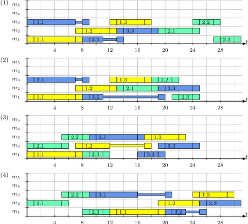
Let us introduce sequence-dependent setup times into the example of Figure 1.2. For each ordered pair of operations executed on the same machine a setup time is defined in Table 1.1. For instance, if operation 2.2 is executed directly after 3.1 on machine m3 then a setup time of 2 occurs, see row 3.1, column 2.2 in block m3.
A solution is depicted in Figure 1.3. The processing sequences on the machines are the same as in the solution of the JS (see Figure 1.2). Setups are depicted by narrow, hatched bars. Due to the setup times, starting and finishing times of the operations have changed and the makespan has increased from 14 to 17.
1.4.2. Release Times and Due Dates
In the JS it is assumed that all jobs are available in the beginning of the planning horizon. In practice, however, jobs may not be able to start at time 0 for various reasons including dynamic job arrivals or prior planning decisions. The earliest time a job can start is called release time.
4 8 12 16 20 24 t m1 m2 m3 3.2 1.1 2.3 2.1 3.3 1.2 3.1 2.2 1.3
Figure 1.4.: A solution of an example with release times and due dates.
Furthermore, a job may have to be finished at some given time, called due date, for instance due to delivery time commitments to customers and planning decisions (e.g. prioritization of the jobs).
For each job, its release time and due date specifies a time window within which its operations should or must be executed. Completion after the due date is generally allowed but such lateness is penalized. A due date that must be satisfied is called deadline (cf. Pinedo [96], p. 14).
Consider time windows in the example of Figure 1.2. Assume that for job 1, 2 and 3, the release time is 7, 6 and 0, and the due date is 23, 16 and 14, respectively. The solution depicted in Figure 1.4 respects these times.
1.4.3. Limited Number of Buffers and Transfer Times
After completion of an operation, a job is either finished, goes directly to its next machine or waits somewhere until its next machine becomes available. Buffers, also called storage places, may be available for the jobs that must wait. If no buffer is available or all buffers are occupied, a job may also wait on its machine, thus blocking it, until a buffer or the next machine becomes available.
Transferring a job from a machine to the next (or to a buffer) needs some time during which both resources are simultaneously occupied. This time is called transfer time.
In the JS it is assumed that an unlimited number of buffers is available, and transfer times are negligible or part of the processing times. In practice, however, the number of buffers is limited for various reasons. Buffers may be expensive or inadequate for technological reasons, or the number of buffers is limited in order to efficiently limit and control work-in-process.
Many systems in practice have limited or no buffers, for example flexible manufac-turing systems [107], robotic cells [30], electroplating lines [73], automated warehouses [62] and railway systems [88].
Consider no buffers and transfer times 0 for all transfers in the example of Figure 1.2. A solution is shown in Figure 1.5. Blockings are depicted by narrow bars filled in the color of the job that is blocking the machine. For example, job 2 waits on machine m2 from time 4 to 6.
12 1.4. EXTENSIONS OF THE CLASSICAL JOB SHOP 4 8 12 16 20 24 t m1 m2 m3 1.1 3.2 2.3 2.1 1.2 3.3 3.1 2.2 1.3
Figure 1.5.: A solution of an example without buffers and with transfer times 0.
4 8 12 16 20 24 t m1 m2 m3 1.1 3.2 2.3 1.2 2.1 3.3 3.1 1.3 2.2
Figure 1.6.: A solution of an example without buffers and with transfer times 1.
Now consider no buffers and transfer times 1 for all transfers in the example of Figure 1.2. A solution is shown in Figure 1.6. Transfers are depicted by bars in the color of the job. Note that the processing sequences on the machines have changed compared to the solution in Figure 1.5 since those sequences are infeasible in case of positive transfer times. Indeed, the three jobs swap their machines at time 6 in the solution with transfer times 0. It is easy to see that such “swaps” are not feasible in the case of positive transfer times.
1.4.4. Time Lags and No-Wait
Consecutive operations in a job are sometimes not just coupled by precedence relations as in the JS, but the time after the end of one operation and the beginning of the next may be restricted by minimum and maximum time lags.
Clearly, a precedence relation between consecutive operations in a job can be mod-eled with such time lags by setting the minimum time lag to 0 and the maximum time lag to infinity (not present). If the minimum time lag is negative, the next operation might start before the previous is finished. If both (minimum and maximum) time lags are 0, the relation is referred to as no-wait, imposing that the job’s next operation has to start exactly when the previous operation is finished. More generally, if the minimum and maximum time lag is equal, then the relation is referred to as fixed time lag or generalized no-wait.
In practice, time lags arise in various industries. Particularly important is this feature if chemical reactions are present (e.g. in the chemical and pharmaceutical sectors [100], semiconductor and electroplating industries [68]), and if properties such as temperature and viscosity have to be maintained (e.g. in the metalworking industry [22]).
4 8 12 16 20 24 t m1 m2 m3 1.1 3.2 2.3 1.2 3.3 2.1 3.1 1.3 2.2
Figure 1.7.: A solution of an example with no-wait relations.
4 8 12 16 20 24 t m1 m2 m3 m4 m5 1.1 3.2 2.1 1.2 3.3 2.2 1.3 2.3 3.1
Figure 1.8.: A solution of an example with routing flexibility.
Consider the example of Figure 1.2 and introduce a no-wait relation between any two consecutive operations in a job. A solution of this example is depicted in Figure 1.7.
1.4.5. Routing Flexibility
In the JS, each operation is processed on a dedicated machine. In practice, however, an operation may be performed by various machines and one of these alternatives must be selected. This feature is commonly called routing flexibility. In a job shop with routing flexibility, not only starting times of the operations, but also an assignment of a machine for each operation must be specified.
Routing flexibility is mainly achieved by the availability of multiple identical ma-chines and by a machine’s capability of performing different processing steps. This feature can be found in almost all industries. Typical examples are multi-purpose plants in process industries [100] and flexible manufacturing systems [72].
Consider the example of Figure 1.2 and duplicate machines m1 and m3, i.e. add two additional machines, called m4 and m5, able to execute operations 1.1, 2.3, 3.2 and 1.3, 2.2, 3.1, respectively. A solution of this example is depicted in Figure 1.8.
14 1.5. OVERVIEW OF THE THESIS 0 1 2 3 4 m1 m2 m3 r1 r2 x rail
Figure 1.9.: The layout of a transportation system.
1.4.6. Transports
After completion of an operation, a job has to be transported to its next machine if this machine is not at the same location as the current machine. In the JS, such transport steps are neglected or included in the processing times. In many practical cases, however, transports need to be considered, e.g. because they take a considerable amount of time, or only a limited number of mobile devices is available to execute the moves.
Mobile devices often interfere with each other in their movements. Typically, inter-ferences arise when these devices move in a common transportation network. Apart from scheduling the processing and transport operations, also feasible trajectories of the mobile devices must be determined in such cases.
In practice, versions of job shop problems with transportation arise in various sec-tors, for example in electroplating plants [73], in the metalworking industry [40], in container terminals [82], and in factories with overhead cranes [5] and robotic cells [35].
Consider the example of Figure 1.2. Introduce the transportation system sketched in Figure 1.9 consisting of robots that transport the jobs from one machine to the next. The robots move on a common rail line with a maximum speed of one. They cannot pass each other and must maintain a minimum distance from each other of one. Machines m1, m2 and m3 are located along the rail at the locations 1, 2 and 3, respectively (measured on the x-axis). There are no buffers available. Transferring a job from a machine to a robot, or vice versa, takes one time unit.
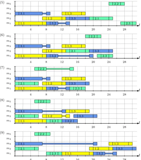
A solution with one and two robots is depicted in Figure 1.10 and 1.11, respectively. The horizontal and vertical axis stands for the time and the location on the rail, re-spectively. The machining operations are depicted as bars at the location representing the location of the corresponding machine. Transport operations are not shown, but can be inferred from the trajectories of the robots that are drawn by lines. Thick line segments indicate that the robot is loaded with a job executing a transport operation, while thin sections correspond to idle moves.
1.5. Overview of the Thesis
In view of the limited applicability of the JS in practice, richer job shop models and general solution methods for these models are needed to bridge the gap between theory and practice. In this thesis, we aim toward closing this gap by proposing a
4 8 12 16 20 24 28 32 36 t x 1 2 3 4 1.1 1.2 1.3 2.1 2.2 2.3 3.1 3.2 3.3 r1
Figure 1.10.: A solution of an example with one robot.
4 8 12 16 20 24 28 32 36 t x 1 2 3 4 1.1 1.2 1.3 2.1 2.2 2.3 3.1 3.2 3.3 r1 r2
16 1.5. OVERVIEW OF THE THESIS
complex job shop model and a solution method that can be applied to a large class of complex job shop problems.
The thesis consists of two parts. In Part I, a general model, called the Complex Job Shop (CJS) model, covering (to some extent) the practical features introduced in Section 1.4 is established and a formulation based on a disjunctive graph is developed in Chapter 2. Based on the disjunctive graph formulation, Chapter 3 develops a heuristic solution method that can be applied to a large class of CJS problems. The approach is a local search based on job insertion and is called the Job Insertion Based Local Search (JIBLS).
In Part II, the CJS model and the JIBLS solution method are tailored and applied to a selection of complex job shop problems obtained by extending the JS with a com-bination of the practical features described in Section 1.4. Some of these problems are known and some have not yet been addressed in the literature. In the known prob-lems, the numerical results obtained by the JIBLS are compared to the best results found in the literature, and in the other problems first benchmarks are established and compared to results obtained by a Mixed Integer Linear Programming (MIP) approach.
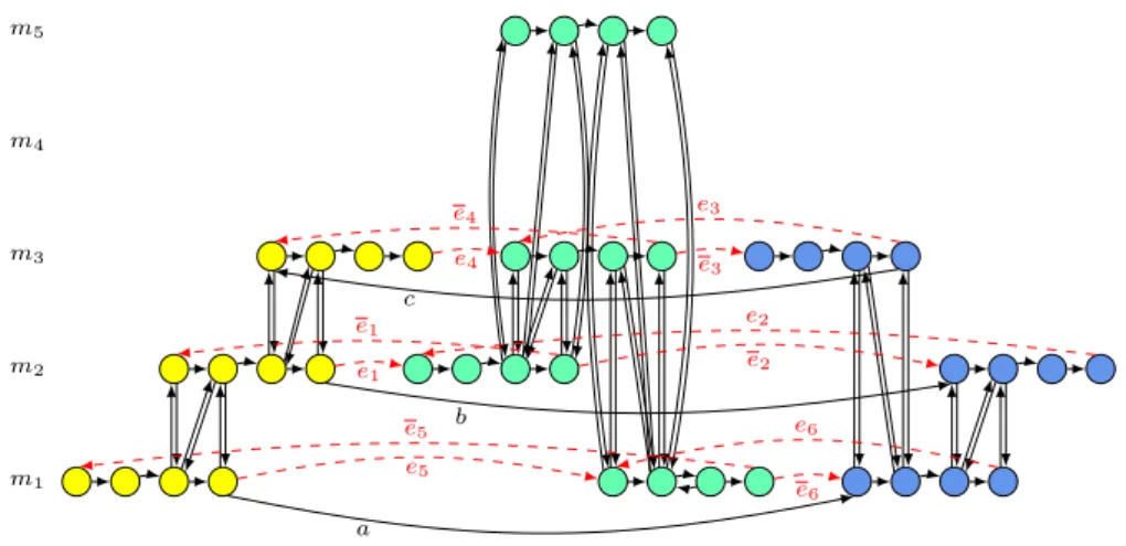
The landscape of the selected complex job shop problems is provided in Figure 1.12. The vertical axis describes features defining the coupling of two consecutive operations in a job (i.e. buffers and time lags), and the horizontal axis provides the other addressed features (i.e. setups, flexibility and transportation). Each problem is represented by a box.
In Chapter 4, an extension of the JS characterized by sequence-dependent setup times and routing flexibility, called the Flexible Job Shop with Setup Times (FJSS), is considered. The FJSS and its simpler version without setup times, called the Flexible Job Shop (FJS), are known problems in the literature.
In Chapter 5, a version of the FJSS characterized by the absence of buffers, called the Flexible Blocking Job Shop with Transfer and Setup Times (FBJSS), is treated. Literature related to the FBJSS is mainly dedicated to its simpler version without flexibility and without setup times, called the Blocking Job Shop (BJS). While the BJS has found increasing attention over the last years, we are not aware of previous literature on the BJS with flexibility and with setup times, except for publication [45]. Chapter 6 addresses instances of FJSS and FBJSS problems where jobs are pro-cessed on machines in a sequence of machining operations and are transported from one machine to the next by mobile devices, called robots, in transport operations. We assume in this chapter that the robots do not interfere with each other, and consider two versions of the problem. In the first version, called the Job Shop with Transporta-tion (JS-T), an unlimited number of buffers is available, and in the second version, called the Blocking Job Shop with Transportation (BJS-T), no buffers are available. While the JS-T is a standard problem in the literature, the BJS-T has not yet been addressed.
Building on the previous chapter, in Chapter 7 we address a version of the BJS-T with robots that interfere with each other in space, and call it the Blocking Job Shop with Rail-Bound Transportation (BJS-RT). The robots move on a single rail line along which the machines are located. The robots cannot pass each other, must maintain
F eatur es unlimited buffers w/o tim e lags w/o buffers w/o ti me lags w/o buffers with tim e lags fixed ti me lags (no-w ait) w/o set ups w/o flexibilit y with setu ps w/o flexibilit y w/o setu ps with fl exibilit y with setups with fl ex ibilit y transp orta tion w/o collisions transp orta tion on a single rail li ne CJS FBJSS FBJS BJSS BJS FJSS FJS JSS JS BJS-T JS-T BJS-R T NWJSS NWJS FNWJSS FNWJS NWJS-T (transitiv e arcs are omitted) Legend Chap. 2-3 Chap. 4 Chap. 5 Chap. 6 Chap. 7 Pub. [20] a b b can b e mo deled as an instance of a w/o: without
18 1.5. OVERVIEW OF THE THESIS
a minimum distance from each other, but can “move out of the way”. Besides a schedule of the (machining and transport) operations, also feasible trajectories of the robots, i.e. the location of each robot at any time, must be determined. Building on the BJS-T and an analysis of the feasible trajectory problem, a formulation of the BJS-RT in a disjunctive graph is derived. Efficient algorithms to determine feasible trajectories for a given schedule are also developed. To our knowledge, the BJS-RT is the first generic job shop scheduling problem considering interferences of robots.
In Figure 1.12, complex job shop problems with fixed time lags, sometimes called generalized no-wait job shop problems, are also illustrated. These problems are not addressed in this thesis. However, the version with setups, called the No-Wait Job Shop with Setup Times (NWJSS) is addressed in the publication [20] and solved by a method that is also based on job insertion, but that is different to the approach taken in the JIBLS.
Complex Job Shop Scheduling
In this part, a general model, called the Complex Job Shop (CJS) model, that cov-ers (to some extent) the practical features introduced in Section 1.4 is established and a formulation based on a disjunctive graph is given. Furthermore, a local search heuristic based on job insertion is developed. It is applicable to a large class of CJS problems, and will be called the Job Insertion Based Local Search (JIBLS).
MODELING COMPLEX JOB SHOPS
2.1. Introduction
In this chapter we develop a complex job shop model that covers the wide range of practical features discussed in the previous chapter: sequence-dependent setup times, release times and due dates, no buffers (blocking), transfers, time lags, and routing flexibility.
The chapter is organized as follows. First, standard formulations of the JS as a disjunctive program, as a mixed integer linear program and as a combinatorial optimization problem in a disjunctive graph are given in Section 2.2. Then, based on the article [42] of Gr¨oflin and Klinkert, a general disjunctive scheduling model is presented in Section 2.3. This model does not “know” jobs and machines. We adapt the model in Section 2.4 by specializing it to capture essential features of the job shop such as machines and job structure, and by extending it to include routing flexibility. The obtained model also captures the aforementioned practical features and will be called the Complex Job Shop (CJS) model.
Graphs will be needed. They will be directed, unless otherwise stated, and the following standard notation will be used. An arc e = (v, w) has a tail (node v), and a head (node w), denoted by t(e) and h(e) respectively. Also, given a graph G = (V, E), for any W ⊆ V , γ(W ) = {e ∈ E : t(e), h(e) ∈ W }, δ−(W ) = {e ∈ E : t(e) /∈ W and h(e) ∈ W }, δ+(W ) = {e ∈ E : t(e) ∈ W and h(e) /∈ W } and δ(W ) = δ−(W )∪δ+(W ). These sets are defined in G, we abstain however from a heavier notation, e.g. δ+G(W ) for δ+(W ). It will be clear from the context which underlying graph is meant. Finally, in a graph G = (V, E, d) with arc valuation d ∈ RE, a path (or cycle) in G of positive length will be called a positive path (or cycle) and a path of longest length a longest path.
22 2.2. SOME FORMULATIONS OF THE CLASSICAL JOB SHOP
2.2. Some Formulations of the Classical Job Shop
A number of formulations of the JS are given in well-known works (e.g. Manne [75], Balas [8], Adams et al. [1]) and in standard textbooks on scheduling (e.g. Blazewicz et al. [11], Brucker and Knust [17], Pinedo [96]). We recall here the disjunctive programming formulation given in Section 1.3, and derive from it standard formulations as a mixed integer linear program and as a combinatorial optimization problem in a disjunctive graph.
2.2.1. A Disjunctive Programming Formulation
Recalling that Q contains all unordered pairs {i, j} of distinct operations i, j ∈ I with mi= mj, the JS can be formulated as the following disjunctive program:
minimize ατ (2.1)
subject to:
αi− ασ ≥ 0 for all i ∈ Ifirst, (2.2)
ατ− αi ≥ di for all i ∈ Ilast, (2.3)
αj− αi ≥ di for all i, j ∈ I consecutive in some job J, (2.4) αj− αi ≥ di or αi− αj≥ dj for all {i, j} ∈ Q, (2.5)
ασ = 0. (2.6)
For explanations we refer the reader to Section 1.3.
2.2.2. A Mixed Integer Linear Programming Formulation
A mixed integer linear programming formulation can be obtained in a straightforward way using the above disjunctive program and introducing a binary variable yijfor each {i, j} ∈ Q, with the following meaning: yij is 1 if operation i is preceding j, and 0 otherwise. Letting B be a large number, the JS problem is the following MIP problem:
minimize ατ (2.7)
subject to:
αi− ασ≥ 0 for all i ∈ Ifirst, (2.8)
ατ− αi≥ di for all i ∈ Ilast, (2.9) αj− αi≥ di for all i, j ∈ I consecutive in some job J, (2.10) αj− αi+ B(1 − yij) ≥ di for all {i, j} ∈ Q, (2.11) αi− αj+ Byij ≥ dj for all {i, j} ∈ Q, (2.12) yij ∈ {0, 1} for all {i, j} ∈ Q, (2.13)
2.2.3. A Disjunctive Graph Formulation
The JS is frequently formulated as a combinatorial optimization problem in a dis-junctive graph. Each operation is represented by a node in this graph. The nodes of two consecutive operations in a job are linked by an arc representing the precedence constraint between these two operations. The nodes of two operations using a com-mon machine are linked by a pair of disjunctive arcs representing the corresponding disjunctive constraint.
Specifically, the disjunctive graph G = (I+, A, E, E , d) is constructed as follows. Each operation i ∈ I+= I ∪ {σ, τ } is represented by a node and identify a node with the operation it represents.
The set of conjunctive arcs A consists of the following arcs representing the set of constraints (2.2)-(2.4) of the disjunctive programming formulation: (i) for each i ∈ Ifirst, an initial arc (σ, i) of weight 0, (ii) for each i ∈ Ilast, a final arc (i, τ ) of weight di, and (iii) for any two consecutive operations i, j in some job J , an arc (i, j) of weight di.
The set of disjunctive arcs E representing constraints (2.5) of the disjunctive pro-gram is given as follows. For any two distinct operations i, j ∈ I with mi = mj, i.e. {i, j} ∈ Q, there are two disjunctive arcs (i, j), (j, i) with respective weights di, dj. The family E consists of all introduced pairs {(i, j), (j, i)} of disjunctive arcs. Definition 1 Any set of disjunctive arcs S ⊆ E is called a selection in G. A selection S is complete if S ∩ D 6= ∅ for all D ∈ E . Selection S is positive acyclic if subgraph G(S) = (V, A ∪ S, d) contains no positive cycle, and is positive cyclic otherwise. Selection S is feasible if it is positive acyclic and complete.
Then, the JS is the following problem:
Among all feasible selections, find a selection S minimizing the length of a longest path from σ to τ in G(S) = (V, A ∪ S, d).
The disjunctive graph formulations given in some articles and textbooks differ slightly from the above formulation.
First, a disjunctive arc pair is sometimes represented by an undirected arc (an edge), and a complete selection is defined by specifying a direction for each edge, asking |S ∩ D| = 1 for all D ∈ E (see Brucker and Knust [17]).
Second, the distinction between cycles and positive cycles is not needed in the JS, as any cycle in G is positive. Consequently, a feasible selection (sometimes called a “consistent” selection) is a complete selection S where G(S) is acyclic (see Adams et al. [1] and Brucker and Knust [17]). Nevertheless, the more general Definition 1 is given here in view of the other, more complex job shop scheduling problems addressed in the sequel.
2.2.4. An Example
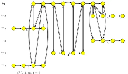
Consider the small JS example introduced in Figure 1.2. The corresponding dis-junctive graph is shown in Figure 2.1. The condis-junctive arcs are colored black, the
24 2.3. A GENERALIZED SCHEDULING MODEL σ 1.1 1.2 1.3 2.1 2.2 2.3 3.1 3.2 3.3 τ m1 m2 m3 0 0 0 6 4 4 4 2 2 6 2 4 6 2 6 2 2 2 4 4 4 4 4 4 4 2 4 6 2 6
Figure 2.1.: Disjunctive graph G of the example.
σ 0 1.1 0 1.2 6 1.3 10 2.1 0 2.2 6 2.3 8 3.1 0 3.2 6 3.3 10 τ 14 m1 m2 m3 0 0 0 6 4 4 4 2 2 6 2 4 6 6 2 4 4 4 2 6 6
Figure 2.2.: Graph G(S) of the feasible selection S corresponding to the schedule from Figure 1.2.
disjunctive arcs are drawn as dashed, red lines and the numbers depict the weights of the arcs.
The feasible selection that corresponds to the schedule from Figure 1.2 is shown in Figure 2.2. The selected disjunctive arcs are drawn as solid, red lines. The starting time of each operation i ∈ I+, i.e. the length of a longest path from σ to i in G(S), is depicted in blue.
This example contains |E | = 9 disjunctive arc pairs, so there are 29 = 512 possi-bilities for selecting exactly one arc from each pair. Only 64 of these selections are feasible. The makespans of all feasible selections are shown in the histogram of Figure 2.3. The best selection has makespan 14 and is the one displayed in Figure 2.2.
2.3. A Generalized Scheduling Model
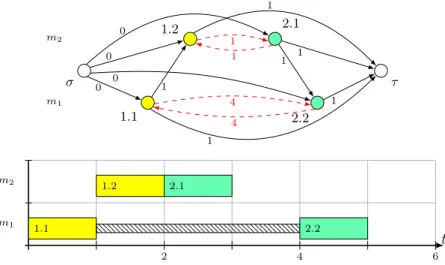
In this section we present a generalized disjunctive scheduling model that can be used to formulate various scheduling problems, among them also the JS. It is based on the article “Feasible insertions in job shop scheduling, short cycles and stable sets” by Gr¨oflin and Klinkert [42].
14 16 18 20 22 24 26 28 30 32 34 0 5 10 15 1 1 4 2 4 12 13 15 6 3 3 Makespan F requency
Figure 2.3.: Makespans of the 64 feasible selections.
2.3.1. A Disjunctive Programming Formulation
Let V be a finite set of events (e.g. starts of operations), σ, τ ∈ V a fictive start and end event, respectively, A ∪ E ⊆ V × V, A ∩ E = ∅, two distinct sets of precedence constraints, and d ∈ RA∪E a weight function. A precedence constraint (v, w) ∈ A ∪ E with weight dvw states that event v must occur at least dvw time units before event w. Precedence constraints of set A and E are called conjunctive and disjunctive precedence constraints, respectively. In contrast to the conjunctive precedence con-straints that always must hold, disjunctive concon-straints must hold if some other dis-junctive constraints in E are violated. Hence, a family of disdis-junctive sets E ⊆ 2E is defined together with E. Each disjunctive constraint is in at least one disjunc-tive set, i.e. S
D∈ED = E. Then, the generalized disjunctive scheduling problem Π = (V, A, E, E , d) is the following problem:
minimize ατ (2.15) subject to: αw− αv≥ dvw for all (v, w) ∈ A, (2.16) _ (v,w)∈D αw− αv≥ dvw for all D ∈ E , (2.17) ασ= 0. (2.18)
Any feasible solution α ∈ RV of Π, also called a schedule, specifies times α
v for all events v ∈ V so that all conjunctive precedence constraints expressed in (2.16) are satisfied and at least one disjunctive precedence constraint of each disjunctive set is satisfied, as expressed in (2.17). The makespan is minimized as expressed in (2.15).
2.3.2. A Disjunctive Graph Formulation
The scheduling problem Π is now formulated in a disjunctive graph G = (V, A, E, E, d), V denoting the node set, A the set of conjunctive arcs, E the set of disjunctive
26 2.3. A GENERALIZED SCHEDULING MODEL
arcs, and d ∈ RA∪E the weights of the arcs. Each event is represented by a node and we identify a node with the event it represents. Each precedence constraint corresponds to an arc (v, w) with weight dvw.
Denote by ΩΠ⊆ RV the solution space of Π. ΩΠcan be described as follows using (complete, positive acyclic, positive cyclic) selections as given in Definition 1.
Let S ⊆ 2E be the family of all feasible selections. Given a selection S, denote by ΩΠ
(S) ⊆ RV
the family of times α ∈ RV satisfying in G(S) = (V, A ∪ S, d):
αw− αv ≥ dvw for all arcs (v, w) ∈ A ∪ S, (2.19)
ασ = 0. (2.20)
Proposition 2 The solution space ΩΠof the scheduling problem Π is ΩΠ= [
S∈S
ΩΠ(S). (2.21)
Proof. i) Consider any S ∈ S and α ∈ ΩΠ(S). By (2.19) and (2.20), (2.16) and (2.18) obviously hold. As selection S is feasible, it is also complete and contains therefore at least one disjunctive constraint (v, w) for all disjunctive sets D ∈ E . Hence by (2.19), (2.17) is satisfied, and α ∈ ΩΠ.
ii) Let α ∈ ΩΠand let S ⊆ E be composed of all disjunctive constraints (v, w) ∈ E that are satisfied by α, i.e. αw− αv ≥ dvw. Obviously, α ∈ ΩΠ(S) for this selection S. We show that S is feasible, i.e. S ∈ S. Indeed, S is complete as α ∈ ΩΠ implies (2.17), i.e. α satisfies at least one disjunctive constraint (v, w) of each disjunctive set D ∈ E . S is also positive acyclic since α ∈ ΩΠ(S) is a feasible potential function in G(S). By a well-known result of combinatorial optimization (see e.g. Cook et al. [26], p.25), G(S) admits a feasible potential function – and hence a solution – if and only if no positive cycle exists in G(S).
Given a feasible selection S ∈ S, finding a schedule α minimizing the makespan is finding α ∈ Ω(S) minimizing ατ. As is well-known, this is easily done by longest path computations in G(S) = (V, A ∪ S, d) and letting αi be the length of a longest path from σ to i for all i ∈ V .
The scheduling problem Π can therefore be formulated as follows:
Among all feasible selections, find a selection S minimizing the length of a longest path from σ to τ in G(S) = (V, A ∪ S, d).
Some remarks concerning the structure of the sets A, E and E are in order. It is assumed that there is a path from node σ to each node v ∈ V and from each node v to node τ in the conjunctive part (V, A, d) of G according to the meaning of σ and τ . Moreover, it is assumed that (V, A, d) is positive acyclic, otherwise no feasible solution exists.
As in [42], the disjunctive sets D ∈ E of the scheduling problems treated in this thesis satisfy:
|D| = 2 for all D ∈ E, (2.22) D ∩ D0= ∅ for any distinct D, D0∈ E, (2.23) D is positive cyclic for all D ∈ E . (2.24) Thus, any disjunctive set D ∈ E is of the form D = {e, e}. Arc e is said to be the mate of e and vice versa. SinceS
D∈ED = E, the disjunctive arc set E is partitioned into |E|/2 disjunctive pairs. Any complete selection S is composed of at least one arc of each pair, and if S is feasible, then by (2.24) it chooses exactly one arc from each pair.
In the disjunctive graph of the JS, the arcs of a disjunctive pair e, e have com-mon end nodes, i.e. they are of the form (v, w), (w, v). In the disjunctive graph of the generalized scheduling problem, a disjunctive arc pair need not be of the form (v, w), (w, v) and may have distinct end nodes.
2.4. A Complex Job Shop Model (CJS)
In the generalized scheduling model, no mention of jobs or machines is made. We adapt this model by specializing it to capture essential features of the job shop such as machines and job structure and by extending it to include routing flexibility. The model includes (to some extent) the features mentioned in Section 1.4 and will be called the Complex Job Shop (CJS) model.
2.4.1. Building Blocks of the CJS Model and a Problem Statement
In the JS, a job is a sequence of operations on machines. After the processing of an operation, the job may be stored somewhere “out of the system” and “comes back” into the system for its next operation. Storage operations and buffers for storing the jobs are not modeled explicitly.
Here we will consider all “machines” used by the jobs from their start to their com-pletion. These machines are not restricted to processors executing some machining, but can also be, for example, buffers for storage operations and mobile devices for transport operations. As in the JS, we assume here that each machine can handle at most one job at any time, and each operation needs one machine for its execution.
In the CJS model, a job can therefore be described as follows. Once started and until its completion, a job is on a machine. After completing an operation, a job might wait on the machine – thus blocking it – until it is transferred to its next machine. While transferring a job, both involved machines are occupied simultaneously.
An operation can be described by the following four steps: i) a take-over step, where the job is taken over from the previous machine, ii) a processing step (e.g. machining, transport or storage), iii) a possible waiting time on the machine, and iv) a hand-over step where the job is handed over to the next machine. The take-over step of an operation must occur simultaneously with the hand-over step of its predecessor
28 2.4. A COMPLEX JOB SHOP MODEL
operation, i.e. the starting time of these steps as well as their duration are the same. Take-over and hand-over steps will be sometimes referred to as transfer steps.
The duration of the processing step and transfer steps are given. The waiting time in step iii) is unknown, but can be limited by specifying a maximum sojourn time allowed on the machine. These times are also called maximum time lags.
We allow for routing flexibility. Each operation needs a machine for its execution. However, this machine is not fixed, but can be chosen from a subset of alternative machines.
We also allow for sequence-dependent setup times between two consecutive opera-tions on a machine, and an initial setup time and a final setup time might be present for each transfer step. The initial setup times, also called release times, specify ear-liest starting times of the transfer steps and the final setup times, also called tails, define minimum times elapsing between the end of the transfer steps and the overall finish time (makespan).
As in the JS, any pair of operations using the same machine must be sequenced, i.e. they cannot be executed simultaneously as a machine can handle at most one job at any time. In addition, we also allow to sequence pairs of transfer steps. The involved machines may not be the same. Such sequencing decisions are for instance needed to model collision avoidance of robots (cf. Chapter 7).
Informally, the CJS problem can be stated as follows. A schedule consists of an assignment of a machine and a starting time of the hand-over, processing and take-over step for each operation so that all constraints described above are satisfied. The objective is to find a schedule with minimal makespan.
2.4.2. Notation and Data
As in the JS, M denotes the set of machines, I the set of operations and J the set of jobs. For each operation i ∈ I, the following notation and data is given.
• i needs a machine for its execution, which can be chosen from a (possibly operation-dependent) subset of alternative machines Mi⊆ M .
• The durations of the take-over, processing and hand-over steps of i are the following. Let h be the job predecessor operation of i and j its job successor operation. For any m ∈ Mi, p ∈ Mh, q ∈ Mj, the duration of the take-over, processing and hand-over step of i is dt(h, p; i, m), dp(i, m) and dt(i, m; j, q), respectively. If i is the first operation of job J , its take-over step is called more appropriately a loading step of duration dld(i, m), and similarly, if i is the last operation of job J , its hand-over step is called an unloading step of duration dul(i, m).
• The maximum sojourn time of i on m ∈ Mi is dlg(i, m). (lg stands for time lag.)
• Let oi be the take-over step and oi the hand-over step of i. Denote by O = {oj, oj: j ∈ I} the set of all transfer steps.
• An initial setup time ds(σ; o, m) and a final setup time ds(o, m; τ ) is given for each transfer step o ∈ {oi, oi} of i.
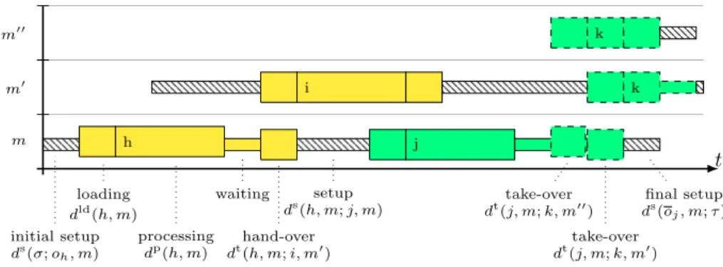
t m m0 m00 h i j k k loading dld(h, m) processing dp(h, m) waiting hand-over dt(h, m; i, m0) initial setup ds(σ; o h, m) setup ds(h, m; j, m) final setup ds(o j, m; τ ) take-over dt(j, m; k, m00) take-over dt(j, m; k, m0)
Figure 2.4.: An illustration of the job structure and our notation.
For any two distinct operations i, j ∈ I and any common machine m ∈ Mi∩ Mj, if j immediately follows i on m, a setup of duration ds(i, m; j, m) occurs on m between the hand-over step oi of i and the take-over step oj of j.
Additionally, let V be the set of pairs of transfer steps that must be sequenced. An element of V has the form {(o, m), (o0, m0)}, o, o0 ∈ O, m, m0 ∈ M, and setup times ds(o, m; o0, m0) and ds(o0, m0; o, m) are given with the following meaning. If transfer step o is executed on machine m and o0 on m0 then they cannot occur simultane-ously, and a minimum time must elapse between them, i.e. o has to end at least ds(o, m; o0, m0) before o0starts, or o0has to end at least ds(o0, m0; o, m) before o starts. We sometimes call V the set of conflicting transfer steps.
In this thesis, set V will be used to model collision avoidance in a job shop setting with multiple mobile devices that move on a common rail (see Chapter 7). If not otherwise stated, we assume V = ∅.
Figure 2.4 illustrates the described structure of the jobs and our notation in a Gantt chart. Four operations h, i, j and k are depicted. Operations h and i are consecutive in one job, and j and k are consecutive in another job. The operations can be executed on the following machines: Mh = Mj = {m}, Mi= {m0}, Mk = {m, m0}. Operation k as well as all involved transfer steps are depicted by dashed lines to indicate the open choice of the machine for k.
Some standard assumptions on the durations are made. All durations are non-negative. For each operation i ∈ I and machine m ∈ Mi, dlg(i, m) ≥ dp(i, m). The difference dlg(i, m) − dp(i, m) is the maximum time the job can stay on machine m after completion of operation i.
Setup times satisfy the following so-called weak triangle inequality (cf. Brucker and Knust [17], p. 11-12). For any operations i, j, k on a common machine m, ds(i, m; j, m) + dp(j, m) + ds(j, m; k, m) ≥ ds(i, m; k, m). The triangle inequality en-sures that setup times between non-consecutive operations on a machine do not be-come active in the disjunctive graph formulation.
It is possible that two operations i, j that are consecutive in a job are on a same machine m ∈ Mi∩ Mj. In this case, both transfer time dt(i, m; j, m) and setup time