• Aucun résultat trouvé

Quantum theory of intersubband polarons

N/A
N/A
Protected

Academic year: 2021

Partager "Quantum theory of intersubband polarons"

Copied!
12
0
0

Texte intégral

(1)

HAL Id: hal-00644634

https://hal.archives-ouvertes.fr/hal-00644634

Preprint submitted on 24 Nov 2011

HAL is a multi-disciplinary open access

archive for the deposit and dissemination of

sci-entific research documents, whether they are

pub-lished or not. The documents may come from

teaching and research institutions in France or

abroad, or from public or private research centers.

L’archive ouverte pluridisciplinaire HAL, est

destinée au dépôt et à la diffusion de documents

scientifiques de niveau recherche, publiés ou non,

émanant des établissements d’enseignement et de

recherche français ou étrangers, des laboratoires

publics ou privés.

Simone de Liberato, Cristiano Ciuti

To cite this version:

(2)

Simone De Liberato and Cristiano Ciuti

Laboratoire Mat´eriaux et Ph´enom`enes Quantiques,

Universit´e Paris Diderot-Paris 7 and CNRS, UMR 7162, 75013 Paris, France

We present a microscopic quantum theory of intersubband polarons, quasiparticles originated from the coupling between intersubband transitions and longitudinal optical phonons. To this aim we develop a second quantized theory taking into account the Fr¨ohlich interaction between phonons and intersubband transitions and the Coulomb interaction between the intersubband transitions themselves. Our results show that the coupling between the phonons and the intersubband transi-tions is extremely intense, thanks both to the collective nature of the intersubband excitation and to the natural tight confinement of optical phonons. Not only the coupling is strong enough to spectroscopically resolve the resonant splitting between the modes (strong coupling regime), but it can become comparable to the bare frequency of the excitations (ultrastrong coupling regime). We thus predict the possibility to exploit intersubband polarons both for applied optoelectronic re-search, where a precise control of the phonon resonances is needed, and also to observe fundamental quantum vacuum physics, typical of the ultrastrong coupling regime.

I. INTRODUCTION

The theory of polarons, the quasiparticles describing electrons moving in a polarizable medium, dates back to the early days of quantum theory1, and it has been an active field of research ever since2. Polarons have been

studied both for three3 and two4,5 dimensional electron

gases, leading to a number of very precise estimates of the quasiparticle mass and energy.

In this paper we will talk of strongly and

ultra-strongly coupled polarons. In polaron theory it is

customary to distinguish between weak coupling6 and

strong coupling7polarons, accordingly to the value of the

Fr¨ohlich coupling constant, that quantifies the strength of the electron-phonon coupling, and that is used as de-velopment parameter in perturbative calculations8. In

this paper anyway we will use the terms strong and ul-trastrong coupling in a different, even if closely related, meaning.

The term strong coupling is commonly used in mod-ern atomic and solid state physics with a rather precise meaning: two systems are strongly coupled if it is possi-ble to resolve, at resonance, the anticrossing due to the coupling. Strong coupling in this latter sense has been predicted9,10 and observed11,12 very early for polaritons coupled to three dimensional plasmons.

The figure of merit of the strong coupling regime is the ratio between the coupling strength, quantified by the so-called vacuum Rabi frequency Ω, and the width of the resonance Γ. If ΩΓ is bigger than one, the two reso-nances are spectroscopically resolved, and the system is in the strong coupling regime. An interesting point to be made is that the fact of whether a system is in the strong coupling regime or not, does not depend on the intrinsic strength of the coupling, but only on the ratio between the coupling and the linewidth; the first observations of the strong coupling regime in atomic systems were made with Rydberg atoms in superconducting cavities, where the strength of the coupling is negligible when compared to the bare frequency of the involved transitions ω, but

where the astounding quality factor of the superconduct-ing cavities allows to resolve the resonant splittsuperconduct-ing13.

It is easy to prove that the value of the ratio Ωω for atomic systems is always much smaller than one, its smallness being linked with the value of the fine struc-ture constant14. Still this severe limitation is valid only

for single particle effects, while collective excitations can beat it thanks to their coherent nature. In a phenomenon reminiscent of the Dicke superradiance15, the strength of the coupling scales as the square root of the number of particles involved, leading to the possibility to obtain val-ues of Ω

ω of the order of one.

This observation has prompted the development of the theory of the so-called ultrastrong coupling regime, that is the regime in which the coupling between two sys-tems is of the same order of their bare frequencies. Such theory was initially developed16,17 in the case of

inter-subband polaritons18 in semiconductor quantum wells,

where it was also observed for the first time19–21. The

ultrastrong coupling regime has since been studied in a lot of different systems, ranging from circuit quan-tum electrodynamics22,23, to organic semiconductors24,

to high mobility electron gases in presence of a perpen-dicular magnetic field25,26.

The interest in such ultrastrong coupling regime is mo-tivated by a whole range of new physics that can be ob-served: from spectral deformations20, to quantum

vac-uum emission phenomena27–29 and even quantum phase

transitions30,31.

This started a race to get the system with the highest value of the light-matter coupling ratio Ωω, with actual record values of 0.12 in superconducting circuits23, 0.16

in organic molecules24, 0.24 in semiconductor quantum wells21 and 0.36 for two dimensional electron gases in

presence of an applied magnetic field26(all coupled to a

confined electromagnetic field).

It is natural at this point to ask how strong the cou-pling of polarons really is. It turns out that, in the case of coupling to collective excitations, it is quite big. Already for the first observation of three dimensional

(3)

plasmon-polaritons11,12we have

ω ≃ 0.2 and values only

marginally smaller were observed for polarons in quan-tum dots32,33.

In this paper we will develop a microscopic theory of the ultrastrong coupling between intersubband tran-sitions and longitudinal optical (LO) phonons in semi-conductor quantum wells, that is the theory of ultra-strongly coupled intersubband polarons. The coupling between intersubband transitions and LO-phonons is rel-evant for a number of optoelectronic applications, as it determines the lifetime of carriers in excited subbands34.

In particular a precise knowledge of LO-phonons inter-subband scattering rates is important in the engineering of heterostructures for quantum cascade lasers35.

Nor-mally optoelectronic devices are designed to avoid being in resonance with optical phonon transitions, due to the high absorption between transverse and longitudinal op-tical phonon frequencies (Restrahlen band). A notable exception is provided by quantum cascade lasers operat-ing near such optical resonances36,37in which instead the

transitions between different subbands are almost reso-nant with LO-phonon modes.

Even if the coupling between intersubband transitions and LO-phonons in semiconductor quantum wells has in-deed received some attention38–40 and intersubband

po-laron resonances have been clearly and unambiguously observed41, the fact that such mixed excitations can be

extremely easily in the strong (or even ultrastrong) cou-pling regime seems overlooked by the community working on intersubband optoelectronic devices. Moreover, to the best of our knowledge, there is no microscopic theory of such excitations, as the spectra of intersubband polarons are normally calculated in an indirect way.

In the Sec. II we explain how our microscopic the-ory differs from the dielectric function approach normally employed to calculate the spectra of intersubband po-larons. In order to build such microscopic theory, we will need to develop an exactly solvable Hamiltonian theory of electron-phonon and electron-electron interactions, heav-ily relying on the concept of superradiant, or coherent, excitation. In Sec. III, we will explain the general con-cept of superradiant excitations, that will then be exten-sively used in Sec. IV to construct the actual theory. In Sec. V we will apply the theory to the case of GaAs quan-tum wells, showing how the ultrastrong coupling regime can be reached even with such relatively weakly polar material. Finally a few considerations on the impact of our results and on possible future developments will be drawn in Sec. VI.

II. LONGITUDINAL EXCITATIONS

Electromagnetism in condensed matter physics is usu-ally studied in the Coulomb gauge. This gauge, while not adapted to high energy physics due to its non-manifestly-covariant form, is particularly well suited to study low energy phenomena, thanks to a natural separation of

dy-namical and instantaneous degrees of freedom. In such gauge we have that, in absence of charges,

div[E(ω)] = 0, (1)

i.e., all propagating waves are transverse. When we con-sider the propagation of an electromagnetic wave in a dispersive medium, Eq. (1) becomes

div[D(ω)] = div[ǫ(ω)E(ω)] = 0, (2)

that is, in a dispersive medium, it is possible to have propagating longitudinal waves at the frequencies for which

ℜ[ǫ(ω)] = 0, (3)

where ℜ indicates the real part. In order to find the frequencies of longitudinal modes it is thus customary to solve Eq. (3) for ω.

If we consider light propagating in a polar material, we can write the equation of the electromagnetic field cou-pled to the transverse optical (TO) phonons and from there we can calculate the dielectric function and finally use it in Eq. (3) to find the frequency of the LO-phonons. An interesting consequence of this approach is that we are calculating the frequency of the LO-phonon mode, con-sidering the coupling of two fields that are not even pled to it, as the propagating electromagnetic field cou-ples to the TO-phonons, not to the LO-phonons. Micro-scopically this stems from the fact that LO-phonons cou-ple to local charges through Coulomb interaction, that is physically the same quantity to which propagating elec-tromagnetic waves couple. Only the particular choice of the Coulomb gauge makes them appear as distinct cou-pling mechanisms.

Polarons are also longitudinal excitations, being par-tially formed of LO-phonons, and as such their energies can be calculated with a simple dielectric function ap-proach as the one sketched just above, if we take into account also the electronic component in the dielectric function. This approach is used, e.g., in Ref. [41]and it indeed gives the right results, also allowing to calculate all the optical observables of the system directly from the dielectric function.

Still physically such approach may appear rather un-satisfactory because, while allowing to calculate a num-ber of physical observables, it completely neglects the microscopic nature of the coupling that creates the po-larons. The polarons are due to the coupling of LO-phonons and electrons (Fr¨ohlich interaction) and in the dielectric function approach, neither the LO-phonons, nor the Fr¨ohlich interaction, are taken explicitly into ac-count.

Apart from this rather formal considerations, missing a microscopic approach makes it difficult, or altogether im-possible, to study what happens in more complex situa-tions, as for example in inhomogeneous samples or when, due to the strength of the coupling, it could become pos-sible to observe exotic phenomena as quantum vacuum effects or quantum phase transitions.

(4)

In the following sections we will develop a detailed mi-croscopic theory for the intersubband transitions coupled to LO-phonons, in the Appendix we will compare the de-veloped theory with the results of the standard dielectric function approach.

III. SUPERRADIANT EXCITATIONS

In 1954 Dicke15noticed that a set of coherently excited

identical dipoles relaxes radiatively much faster than a single, isolated dipole. This is due to the phenomenon of superradiance: N identical dipoles behave as a single collective dipole√N times bigger.

The reason of such collective enhancement can be un-derstood considering that, being all the dipoles identi-cal, all the transitions are degenerate and a simple basis change allows us to describe the system of N dipoles as a single superdipole coupled to the electromagnetic field and N − 1 other modes that are not coupled to the field. The particular superposition that couples to the field (usually called bright mode) thus concentrates all the oscillator strength and has a dipole √N times big-ger.

The concept of superradiance has been thoroughly ap-plied to the study of intersubband polaritons18,42–44 in

microcavity embedded doped quantum wells. In quan-tum wells the confinement of electrons along the growth direction splits the electron bands, giving rise to multiple parallel subbands. Being the subbands parallel, and be-ing the electromagnetically induced transitions between them almost vertical (the wavevectors of the photons are negligible compared to the ones of the electrons), the sit-uation is very similar to the one considered initially by Dicke. The N electrons that populate the lower con-duction subband can jump vertically in the excited one and indeed can be considered as N independent dipoles. As expected16,17, in these systems the strength of the

coupling between light and matter is proportional to the square root of the number of electrons in the quantum well.

In this paper we will not consider the coupling of inter-subband transitions with light, but we will study instead their coupling with longitudinal optical phonons, consid-ering also the role of Coulomb electron-electron interac-tion. Such couplings are extremely rich and, in order to limit the complexity of our investigation, we will need to determine which scattering channels are dominant and which are negligible. Given that, in general, if N elec-trons undergo a certain transition in a coherent way the

strength of the coupling is enhanced by a factor √N,

transitions involving a macroscopic number of electrons will be treated exactly, while the others (involving only few electrons ) will be treated perturbatively (or ignored altogether).

The degree of collective enhancement of a scattering process will be evaluated looking at the number of elec-trons that can participate to the process given fixed

FIG. 1: a) An example of collective transition: an intersub-band transition with small transferred momentum. b) An ex-ample of non-collective transition: an intrasubband transition with small transferred momentum in which most of the single particle transitions are Pauli blocked. c) An example of non-collective transition: an intrasubband transition with large transferred momentum. The extrema of the energy spread of single particle transitions are shown explicitly.

amounts of transferred impulsion and energy. In Fig. 1 we show a few illustrative examples. Panel (a) repre-sents a transition from the first to the second subband, with a negligible amount of transferred momentum. All electrons can undergo this transition approximately at the same energy. This process will thus benefit from a large superradiant enhancement factor, proportional to the square root of the total number of the electrons in the gas. Panel (b) and (c) represent two possible transitions within the first subband. In panel (b) the transferred momentum is much smaller than the Fermi momentum ~kF and the majority of electrons, being Pauli blocked, do not participate to the process. In panel (c) the trans-ferred momentum is of the order of 2~kF, the minimum

to allow all the electrons to undergo a transition avoiding Pauli blocking. Anyway there is a large energy spread be-tween the different single electron transitions. Electrons on the two opposite borders of the Fermi sea, with initial

momenta ±~kF parallel to the transferred momentum,

have initially the same energy ~2k2F

2m∗ = EF, where m ∗ is

the electron effective mass and EF the Fermi energy.

Af-ter the transition they will end up with final momenta of ~kF and 3~kF, corresponding to final energies

~2k2 F 2m∗ = EF

and 9~2k2F

2m∗ = 9EF respectively. This implies that, even if

the transition is not blocked, only a small fraction of the single electron transitions can be resonant at the same time. In both cases, given that only few electrons can participate to the collective transitions, the superradiant

(5)

enhancement factor will be small.

IV. THEORETICAL FRAMEWORK A. Free fields

We will consider a symmetric quantum well of length LQW in a bulk of height LBK, S will be the surface of the

sample. For the moment, we will limit ourselves to the case of a single quantum well, the general case of multiple quantum wells will be addressed later in this Section.

The quantum well is supposed to be doped in such a way that its Fermi level is between the first and the second conduction subbands, separated between them by the intersubband gap energy ~ω12.

We will develop our theory using a zero temperature formalism (T = 0), anyway our results will remain quan-titatively accurate while the thermal population of the second subband remains negligeable. Depending on ma-terial parameters and doping level, this could imply the necessity to perform experiments in different kinds of cryogenic environments.

Electron states will be indexed by the subband index j and by the value of the in-plane wavevector k. Their wavefunctions will be given by

ψj,k(ρ, z) = χj(z)

eikρ

S, j= 1, 2, (4)

where, for simplicity, we will choose χj(z) to be real and,

due to the symmetry of the quantum well, the χj(z) have

well defined and opposite symmetry. Wavefunctions in Eq. (4) are chosen as basis for second quantization, the creation operator for an electron in the state described by Eq. (4) will be denoted as c†j,k. The free Hamiltonian of electron gas in the two considered subbands thus reads

Hel= X j={1,2},k ~ωj(k)c† j,kcj,k, (5) where ω1(k) = ~2k2 2m∗ and ω2(k) = ω1(k)+ω12. In Eq. (5),

as well as in the rest of this paper, we will omit the elec-tron spin index. This is justified by the fact that all inter-actions we consider are spin conserving. Given that we will consider only in-plane wavevector exchanges q much smaller than the typical electron wavevector k, we can make the approximation ωj(k + q) ≃ ωj(k), and

intro-duce the operators describing intersubband transitions with a well defined and dispersionless energy ~ω1216,17

b†q = 1 √ N X k c†2,k+qc1,k, (6) bq = 1 √ N X k c†1,kc2,k+q,

where N is the number of electrons in the quantum well. The b†

qoperators are bosonic in the dilute regime45, that

is, if there are n of such excitations in the system [bq, b

q′] = δq,q′+ O(

n

N) ≃ δq,q′. (7)

Using Eq. (6) we can rewrite the Hamiltonian of the free electron gas in Eq. (5) in terms of bosonic intersub-band excitations

Hel=

X

q

~ω12bqbq. (8)

In this work we are interested in the resonant case in which ω12 is equal, or close, to the LO-phonon

fre-quency ωLO. We can thus neglect confinement

ef-fects on the phonons and consider bulk values for their frequencies46,47. We will thus describe LO-phonons by means of the three dimensional boson operators dq,qz

[dq,qz, d †

q′,qz] = δq,q′δqz,qz′, (9)

indexed by their in-plane and out-of-plane wavevectors. While we know that LO-phonon modes are confined in-side the quantum well, we do not need to impose this constraint in the mode definition because, as we will see, intersubband transitions end up coupling with linear su-perpositions of phonon modes that are anyway confined inside the quantum well. We will consider only the case of one single longitudinal optical branch, the expansion to the case of multiple branches not presenting any fun-damental difficulty.

Moreover, we are interested only in phonons with small plane wavevectors (in order to couple with coherent in-tersubband excitations), we can thus ignore phonon dis-persion and write the free phonon Hamiltonian as

Hph =

X

q,qz

~ωLOd†q,qzdq,qz. (10)

B. Electron phonon interaction

Interaction between electrons and LO-phonons can be described using the Fr¨ohlich Hamiltonian3

HF r= s ~ωLOe2 2ǫ0ǫρSLBK X q,qz e−i(qρ+qzz) pq2+ q2 z d†q,qz + h.c., (11) where 1 ǫρ = 1 ǫ∞ − 1 ǫs , (12)

and ǫs and ǫ∞ are respectively the static and high

fre-quency dielectric constants47.

The Hamiltonian in Eq. (11) can be written in sec-ond quantization (neglecting incoherent intrasubband scattering34) as HF r = s ~ωLOe2 2ǫ0ǫρSLBK X q,qz F(qz) pq2+ q2 z (13) (d†q,qz+ d−q,−qz)(c † 1,kc2,k+q+ c † 2,k−qc1,k),

(6)

where we have defined F(q) =

Z

dzχ1(z)χ2(z)e−iqz. (14)

From Eq. (13) we see that, due to the three dimen-sional character of the LO-phonons47, each electronic

transition couples to multiple phonon modes, indexed by different values of the wavevector along the growth direc-tion. It is thus convenient to introduce second quantized operators corresponding to the particular linear super-position of phonon modes that are coupled to electronic transitions rq† = √1 A X qz F(qz)d†q,qz pq2+ q2 z , rq = 1 √ A X qz ¯ F(qz)dq,qz pq2+ q2 z , (15)

whose spatial wavefunctions along the z axis is ϕq(z) = 1 √ ALBK X qz F(qz)eiqzz pq2+ q2 z . (16)

From Eqs. (16) and (14) we see that the intersubband transitions naturally couple to phonon modes localized inside the quantum well (it is easy to verify that ϕq(z)

vanishes to the first order in q if z is outside the common support of χ1and χ2).

The normalization factor A can be fixed imposing bosonic commutation relations to the r†

q operators [rq, rq†′] = 1 A X qz,q′z F(qz)F (−q′z) q (q2+ q2 z)(q′2+ qz′ 2)[dq,qz, d † q′,qz′] = δq,q′LBKI(q) 2Aq , (17) and thus A = LBK 2 I(q) q , (18)

where we have defined I(q) =

Z

dzdz′χ1(z)χ2(z)χ2(z′)χ1(z′)e−q|z−z ′|

. (19) We can thus write Hamiltonians in Eq. (10) and Eq. (13) in term of coherent r† q and b†q operators as Hph = X q ~ωLOr†qrq, (20) and HF r = X q s N2DEG~ωLO e2 4ǫ0ǫρ I(q) q (b † q+ b−q)(rq+ r†−q),

FIG. 2: a) Graphical representation of the scattering channel Vimnj

q . Two electrons in subbands j and n, with momenta k

and k′

are scattered into subbands i and m, with momenta k+ q and k′− q respectively.

where

N2DEG=

N

S, (21)

is the density of the two dimensional electron gas inside the quantum well. In order to pass from Eq. (10) to Eq. (20), we are neglecting higher order phonon modes confined inside the quantum well. This is justified by the fact that we limit ourselves to long-wavelength modes.

C. Resonant Electron-Electron interaction

In order to treat the Coulomb electron-electron in-teraction we start by the second quantized form of the Hamiltonian describing the Coulomb interaction48 (see

Fig. 2 (a) for a graphical representation of the interac-tion coefficients) Hc= 1 2 X i,j,m,n=1,2 X q,k,k′ Vimnj q c † i,k+qc † m,k′−qcn,k′cj,k, (22) where Vqimnj = e 2 2ǫ0ǫ∞q Z dzdz′χi(z)χj(z)χm(z′)χn(z′)e−q|z−z ′| , (23) is the two dimensional Coulomb matrix element. It is important to notice that in Eq. (23) we used the high

(7)

frequency dielectric constant ǫ∞instead of the static one.

This is due to the fact that ǫs includes the effect of the

coupling to LO-phonons, that is already treated exactly in the Hamiltonian.

Due to the symmetry of the wavefunctions, a certain number of matrix elements in Eq. (23) can be seen to be zero, in particular all the matrix elements with an odd number of 1 and 2 indices

Vq1112 = V1121

q = Vq1211= Vq2111= 0, (24)

Vq2111 = Vq2212= Vq2122= Vq1222= 0. The other elements can be evaluated as

Vq1122 = Vq1212= Vq2121= Vq2211= e2I(q) 2ǫ0ǫ∞q , (25) Vq1221 = V2112 q = e2 2ǫ0ǫ∞q Z dzdz′χ21(z)χ22(z′)e−q|z−z ′| , Vq1111 = e 2 2ǫ0ǫ∞q Z dzdz′χ21(z)χ21(z′)e−q|z−z ′| , Vq2222 = e 2 2ǫ0ǫ∞q Z dzdz′χ22(z)χ22(z′)e−q|z−z ′| ,

where I(q), defined in Eq. (19), is same integral we en-countered studying the electron-phonon Fr¨ohlich interac-tion.

The four distinct nonzero possible values of the matrix elements correspond to different kinds of scattering pro-cesses. In Fig. 2 (b) a graphical representation for each of these processes is shown.

It is important at this point to notice a major differ-ence between the elements in the first line of Eq. (25) and the others. The elements in the first line (upper left subpanel in Fig. 2 (b)) represent intersubband exci-tations: each electron is scattered from one subband to the other. Such processes, responsible for the depolariza-tion shift48, describe a superradiant process in the sense

defined in Sec. III, that is, at least for small values of q, a great number of electrons can coherently undergo the same transition, approximately at the same energy. This is not the case for the interactions described in the other lines of Eq. (25), that instead describe intrasub-band excitations that, either due to Pauli blocking or to the non-flat energy dispersion, involve only few electrons (see Fig. 1).

The discussion in Sec. III thus implies that the

strength of the terms in the first line of Eq. (25) strongly dominates over the others due to the superradiant en-hancement. For this reason we have to treat them ex-actly in an Hamiltonian formalism, while we can limit ourselves to treat the others within a perturbative ap-proach.

Here we will thus construct an exact, Hamiltonian ap-proach, to treat the effect of the depolarization shift terms, neglecting the others. We will analyze later the effect of the intrasubband terms.

Le us start to rewrite the depolarization shift part of Eq. (22) in a more useful form

Hc = X q,k,k′ e2I(q) 4ǫ0ǫ∞q  c†1,k+qc†1,k′−qc2,k′c2,k+ c†1,k+qc † 2,k′−qc1,k′c2,k+ c†2,k+qc † 1,k′−qc2,k′c1,k+ c†2,k+qc † 2,k′−qc1,k′c1,k  = X q,k,k′ e2I(q) 4ǫ0ǫ∞q  c†1,k+qc2,kc†1,k′−qc2,k′+ c†1,k+qc2,kc†2,k−qc1,k′+ c†2,k+qc1,kc†1,k−qc2,k′+ c†2,k+qc1,kc†2,k−qc1,k′  +X q N e2I(q) 4ǫ0ǫ∞q . (26)

We see from Eq. (26) that, thanks to its collective, super-radiant nature, the depolarization shift can be naturally written in terms of the bosonic intersubband excitations defined in Eq. (6) as Hc= X q N2DEG e2 4ǫ0ǫ∞ I(q) q (b † q+ b−q)(b † −q+ bq), (27)

where we have neglected the last constant term, that sim-ply shifts the ground state energy.

D. Residual Electron-Electron interaction

We showed how it is possible to treat exactly the depo-larization shift effect in a bosonic excitation formalism. It remains to study the effect of the residual Coulomb contributions due to the intrasubband terms in the last three lines of Eq. (25) (schematized in the last three panels of Fig. 2 (b)).

An important result due to Lee and Galbraith49,50, is

that such intrasubband terms do not contribute to the screening of the intersubband ones at the level of the random phase approximation (RPA). This can be seen

(8)

writing the Dyson equation for the dynamically screened Coulomb potential51 Vq(ω) Vqimnj(ω) = Vqimnj+ X rs VqirsjΠsr q (ω)Vqsmnr(ω), (28)

where Πsr(q, ω) is the RPA polarization function. In the

case of an intersubband contribution (e.g. V1122

q ), Eqs.

(24) and (25) imply that Vq1122(ω) = Vq1122+ X rs Vq1rs2Πsrq (ω)Vqs12r(ω) (29) = Vq1122+X r6=s Vq1rs2Πsr q (ω)V s12r q (ω) = V1122 q + Vq1122(Π12q (ω) + Π21q (ω))Vq1122(ω). We have thus Vq1122(ω) = Vq1122 1 − V1122 q (Π12q (ω) + Π21q (ω)) , (30)

from which we see that the intrasubband Coulomb terms (V1111

q ,Vq2222, Vq1221 and Vq2112) do not intervene in the

renormalization of the intersubband terms.

An analogous reasoning can be done for the phonon-electron interaction. Calling Mq,qz and Mq,qz(ω) the

bare and screened version of the potential defined in Eq. (13), we have the Dyson equation

Mq,qz(ω) = Mq,qz+ X rs Vq1mn2Πsr q (ω)Mq,qz(ω) (31) = Mq,qz+ V 1122 q (Π 12 q (ω) + Π 21 q (ω))Mq,qz(ω),

and we have thus the formula for the screened potential Mq,qz(ω) =

Mq,qz

1 − V1122

q (Π12q (ω) + Π21q (ω))

. (32)

Being the RPA screening only due to terms that are ex-actly treated in the Hamiltonian, we can thus neglect the screening due to the two dimensional electron gas.

E. Hopfield-Bogoliubov Hamiltonian

Putting together Eqs. (8), (21) and (27) we arrive to the full Hamiltonian for the intersubband transitions-LO-phonons system H = X q ~ω12bqbq+ ~ωLOrqrq (33) + s N2DEG~ωLO e2 4ǫ0ǫρ I(q) q (b † q+ b−q)(r † −q+ rq) +N2DEG e2 4ǫ0ǫ∞ I(q) q (b † q+ b−q)(b † −q+ bq).

The Hamiltonian in Eq. (33) can be rewritten in a

more compact form by introducing the intersubband

transitions-LO-phonons coupling constant Ω and the de-polarization shift constant D

Ω = s N2DEGωLO e2 4ǫ0ǫρ~ I(q) q , (34) D = N2DEG e2 4ǫ0ǫ∞ I(q) q ,

where we have dropped the dependences over the wavevector as we are interested in the long wavelength limit (from Eq. (19) we can verify that limq→0I(q)q tends

to a constant value).

Using Eq. (34), Eq. (33) can be written as

H = ~X q ω12b†qbq+ ωLOr†qrq+ Ω(b†q+ b−q)(r † −q+ rq) +D(b†q+ b−q)(b † −q+ bq), (35)

that can be cast in matrix form as

H =~ 2 X q ˆ v†qη Mqvˆq, (36)

where the column vector of operators ˆvq is defined as

ˆ

vq= [bq, rq, b†−q, r †

−q]T, (37)

η is the diagonal metric

η= diag[1, 1, −1, −1], (38)

and the Hopfield-Bogoliubov52 matrix M

q is defined as Mq=    ω12+ 2D Ω 2D Ω Ω ωLO Ω 0 −2D −Ω −ω12− 2D −Ω −Ω 0 −Ω −ωLO   . (39)

Diagonalizing the matrix in Eq. (39) will yield the frequencies of the normal modes of the system ω±, that

are usually called polarons32,33. In our case we will name

them more properly intersubband polarons, because the electronic part of the mixed excitation is given by an intersubband transition.

It is interesting to notice that, from Eq. (34), we can write the Coulomb coefficient D as

D = Ω 2 ωLO ǫρ ǫ∞ ≥ Ω2 ωLO . (40)

As it has recently been shown in Ref. [53], Eq. (40) implies that it is impossible to observe a Dicke phase transition in the system we are considering, regardless of the strength of the coupling.

F. Multiple Quantum Wells

Until now we considered the case of a single quantum well. This choice has been motivated by the fact that,

(9)

as we will show, the presence of multiple quantum wells does not modify our results.

Given that we are considering rather large quantum wells (in order for the transition to be resonant with the LO-phonon mode), the optical phonon spectrum is not modified47and the optical phonon modes we consider are

confined in each quantum well.

This is a rather important difference between the inter-subband polaron case we consider in this paper and the physics of intersubband polaritons. For intersubband po-laritons, the electromagnetic mode coupled to the inter-subband transitions extends over all the quantum wells in the structure. It thus couples to all the electrons, regard-less of the quantum well they are in. This means that the only meaningful parameter for intersubband polari-tons is the total density of electrons, and the light-matter coupling thus scales aspnQWN2DEG, where nQW is the

number of quantum wells inside the microcavity. In the present case instead, being the phonon modes confined inside each quantum well, electrons in different quantum wells are completely decoupled. This can also be inferred from the coupling integral in Eq. (23). This integral does vanish, at least in the long wavelength limit (first order in q), if the wavefunctions for the two integra-tion variables z and z′ do not have a common support,

i.e., if the two interacting electrons are in different quan-tum wells.

This means that, contrary to the intersubband polari-ton case, the intersubband polaron interaction scales only

as √N2DEG and growing multiple quantum wells in the

same sample will not increase the coupling.

V. RESULTS

In order to obtain some numerical predictions from Hamiltonian in Eq. (35), we need to fix a few parameters concerning the material and the quantum well.

For sake of simplicity we will consider the quantum well to be correctly approximated by a rectangular, infinite potential well of length LQW. We thus have

~ω12 = 3~

2π2

2m∗L2 QW

, (41)

and the electronic and phononic modes profiles are given by χ1(z) = s 2 LQW sin( πz LQW ), (42) χ2(z) = s 2 LQW sin( 2πz LQW ), ϕ0(z) = s 16 5LQW sin3( πz LQW ), (43)

inside the quantum well and zero outside. As explained in Sec. IV, we see here explicitly that the intersubband transitions couple to a linear superposition of phonon modes that is localized inside the quantum well (the cubic sinus in the third line of Eq. (42) comes from the integral of the two first two, as can be verified performing the integral in Eq. (16)).

Inserting Eq. (42) into Eq. (19) and performing the integral we have

lim

q→0I(q) →

10

9π2qLQW. (44)

In Fig. 3 we plot the normalized coupling ωΩLO as a

function of the two dimensional electron gas, for a GaAs quantum well. In the inset of Fig. 3 we instead present

a comparison of the values of Ω

ωLO, at room

tempera-ture, for different semiconductors of the III-V and II-VI groups54, as a function of the respective LO-phonon

en-ergies, for a reference doping N2DEG= 1012cm−2.

In Fig. 4 there is a plot of the intersubband polaron fre-quencies ω± as a function of the intersubband frequency

ω12, in GaAs, for N2DEG= 1012cm−2. Notice that, due

to the effect of Coulomb interaction, the resonant anti-crossing is not at ω12 = ωLO but at a lower frequency.

In the inset of the same figure we plot the same quan-tity as a function of the electron density. The quantum well length LQW has been chosen in this case to have the

two uncoupled modes at resonance (ω12 = ωLO, that is

LQW ≃ 23nm).

It is clear from the figure that intersubband polarons are not only strongly coupled, having coupling constants much larger than their linewidth (usual linewidths be-ing not bigger than a few meV), but they are indeed in the ultrastrong coupling regime, with values of the renor-malized couplingωΩLO comparable or larger than the best

ones reported in the literature21. For physically

realiz-able levels of doping, coupling values of a few tenths of the bare frequency of the excitation ωLO are predicted

in GaAs, and it seems that values much larger can be obtained using more polar materials. The reason of such large coupling can be found in the superradiant nature of intersubband excitations and in the natural confine-ment of the phonons inside the quantum well, that gives an extremely small mode volume, when compared with what can be obtained with photonic microcavities.

The consequences of our results can be multiple, both for fundamental and applied research. On the fundamen-tal side, intersubband polarons could become a new labo-ratory to test quantum vacuum physics, typical of the ul-trastrong coupling regime28. On the applied side our

the-ory can be naturally exploited in the study of quantum cascade lasers working in or near the Restrahlen band. It can, for example, help explaining the anticrossing ob-served in Ref. 36, near the LO-phonon frequency. More-over the capability to strongly modify the LO-phonon spectrum could have an impact on the performances of optoelectronic devices, as the electron-LO-phonon scat-tering rate determines the lifetime of carriers in excited

(10)

0 0.2 0.4 0.6 0.8 1 0 0.05 0.1 0.15 0.2 20 30 5040 0.1 0.2 0.3 0.4 0.5 ZnSe CdTe GaAs InP InAs InSb

N

2DEG

(×10

12

cm

−2

)

ωLO(meV )

/

ω

L O Ω / ωL O

FIG. 3: Normalized coupling Ω

ωLO in GaAs as a function of the

doping density N2DEG. Inset: the same quantity as a function

of the LO-phonon frequency ωLO for different materials, for

N2DEG= 1012cm−2. 0 0.2 0.4 0.6 0.8 1 0 0.2 0.4 0.6 0.8 1 1.2 1.4 1.6 0 10.5 0.8 1 1.2 1.4 1.6

ω

12

LO N2DEG(×1012cm −2 )

ω

±

/

ω

L O ω± / ωL O

FIG. 4: Intersubband polaron frequencies ω± as a function

of the intersubband frequency ω12for GaAs. Inset: the same

quantity as a function of the doping for ω12= ωLO.

subbands34.

VI. CONCLUSIONS

In this paper we have developed a microscopic the-ory of intersubband polarons, mixed excitations result-ing from the couplresult-ing between intersubband transitions in doped quantum wells and LO-phonons. We took into account the electron-electron Coulomb interaction and we were able to treat exactly the resulting depolarization

shift. We proved that intersubband polarons can be in the ultrastrong coupling regime, reaching extremely high values of the coupling constant. We critically discussed the relevance of our result both for fundamental and ap-plied research.

VII. ACKNOWLEDGMENTS

We would like to thanks D. Hagenm¨uller, M. Zaluzny, P. Nataf, L. Nguyen, J. Restrepo, C. Sirtori and Y. Todorov for useful discussions and comments.

Appendix: Comparison with dielectric function theory

As explained in Sec. II, the dispersion of intersubband polarons can be calculated by solving Eq. (3) for the dielectric function of the coupled quantum well-lattice system. In order to test our theory we will compare this approach, following what done in Ref. [41], with the microscopic one we developed in this manuscript.

The total dielectric function of the system is given by21,41 ǫ(ω) = ǫ∞ ω2− ω2LO ω2− ω2 T O+ iω0+ − ǫ∞ ω2P ω2− ω2 12+ iω0+ , (45) where ω2P =2ω12d 2 12N2DEG ~ǫ0ǫ∞LQW , (46)

is the plasma frequency of the two dimensional electron gas and d12 is the intersubband dipole

d12= e Z dzχ1(z)zχ2(z). (47) The equation ℜ[ǫ(ω)] = 0, (48) thus reads ω4− ω2(ω2 LO+ ω122 + ωP2) + ω2LOω122 + ω2T Oω2P = 0. (49) Note that Eq. (45) refers to the dipolar function along the z direction. In order to recover the same result from our microscopic approach, we will thus have to consider only q = 0 phonons. Moreover, the use of a simple di-electric function theory, requires to have an homogeneous medium. This is equivalent to consider only the mode with qz→ 0, that is, from Eqs. (14) and (47)

F(qz)

pq2+ q2 z

(11)

Following exactly the same procedure done in Sec. IV, but with the F (q) defined in Eq. (50) and considering only the qz→ 0 mode, we get

Ω = s

N2DEGωLOd212

2ǫ0ǫρLQW~

, (51)

and thus, from Eq. (40)

D = N2DEGd

2 12

2ǫ0ǫ∞LQW~

. (52)

In order to obtain the polaronic eigenfrequencies we have to diagonalize the matrix in Eq. (39) using the coupling coefficients for the homogeneous limit defined in Eqs. (51) and (52). We thus obtain the secular equation

ω4− ω2(ω2

LO+ ω122 + 4Dω12) (53)

LO2 ω212+ 4Dω12ωLO2 − 4Ω2ω12ωLO= 0,

that, using Eqs. (52) and (46) can be put into the form ω4− ω2(ωLO2 + ω212+ ωP2) + ω 2 LOω 2 12+ ωP2ω 2 LO ǫ∞ ǫs = 0. (54) Equating the coefficients of Eqs. (49) and (54), we obtain

ω2T O = ωLO2

ǫ∞

ǫs

, (55)

that is the well known Lyddane-Sachs-Teller relation47.

We have thus proved that the homogeneous version of our theory gives the same results as the homogeneous dielectric function approach.

It is anyway important to notice that the homoge-neous limit in not exact, as a quantum well is, by defi-nition, non-homogeneous. Ignoring the higher qz modes

leads to underestimate the intersubband dipole of a fac-tor roughly equal to√2.

1

L. D. Landau, Phys. Z. Sovjet 3, 664 (1933).

2

J. T. Devreese, Encyclopedia of Applied Physics 14, 383 (1996).

3

H. Fr¨ohlich, Adv. Phys. 3, 325 (1954).

4

X. G. Wu, F. M. Peeters and J. T. Devreese, Phys. Rev. B 34, 2621 (1986).

5

F. M. Peeters and J. T. Devreese, Phys. Rev. B 36, 4442 (1987).

6 R. P. Feynman, Phys. Rev. 97, 660 (1955). 7

S. J. Miyake, J. Phys. Soc. Japan 38,181 (1975).

8

G. D. Mahan, Many Particle Physics, Springer (2000).

9

B. B.Varga, Phys. Rev. D7, A1896 (1965).

10

K. S. Singwi and M. P. Tosi, Phys. Rev. 147, 658 (1966).

11

A. Mooradian and A. L. McWhorter, Phys. Rev. Lett. 19, 849 (1967).

12

C. G. Olson and D. W. Lynch, Phys. Rev. 177, 1231 (1968).

13

S. Haroche and J.-M. Raimond, Exploring the Quantum: Atoms, Cavities, and Photons, Oxford University Press (2006).

14

M. Devoret, S. Girvin, R. Schoelkopf, Ann. Phys. (Leipzig) 16, 767 (2007).

15

R. H. Dicke, Phys. Rev. 93, 99 (1954).

16

C. Ciuti, G. Bastard and I. Carusotto, Phys. Rev. B 72, 115303 (2005).

17

C. Ciuti and I. Carusotto, Phys. Rev. A 74, 033811 (2006).

18

D. Dini, R. Kohler, A. Tredicucci, G. Biasiol and L. Sorba, Phys. Rev. Lett. 90, 116401 (2003).

19

G. G¨unter, A. A. Anappara, J. Hees, A. Sell, G. Biasiol, L. Sorba, S. De Liberato, C. Ciuti, A. Tredicucci, A. Leiten-storfer and R. Huber, Nature (London) 458, 178 (2009).

20 A. A. Anappara, S. De Liberato, A. Tredicucci, C. Ciuti,

G. Biasiol, L. Sorba and F. Beltram, Phys. Rev. B 79, 201303 (2009).

21

Y. Todorov, A. M. Andrews, R. Colombelli, S. De Liberato, C. Ciuti, P. Klang, G. Strasser and C. Sirtori, Phys. Rev. Lett. 105, 196402 (2010).

22

J. Bourassa, J. M. Gambetta, A. A. Abdumalikov, Jr., O.

Astafiev, Y. Nakamura and A. Blais, Phys. Rev. A 80, 032109 (2009).

23 T. Niemczyk, F. Deppe, H. Huebl, E. P. Menzel, F. Hocke,

M. J. Schwarz, J. J. Garcia-Ripoll, D. Zueco, T. H¨ummer, E. Solano, A. Marx and R. Gross, Nat. Phys. 6, 772 (2010).

24

T. Schwartz, J. A. Hutchison, C. Genet and T. W. Ebbe-sen, Phys. Rev. Lett. 106, 196405 (2011).

25

D. Hagenm¨uller, S. De Liberato and C. Ciuti, Phys. Rev. B 81, 235303 (2010).

26

G. Scalari, C. Maissen, D. Turcinkov´a, D. Hagenm¨uller, S. De Liberato, C. Ciuti, D. Schuh, C. Reichl, W. Wegschei-der, M. Beck and J. Faist, arXiv:1111.2486.

27

M. Kardar and R. Golestanian, Rev. Mod. Phys. 71, 1233 (1999).

28

S. De Liberato, C. Ciuti and I. Carusotto, Phys. Rev. Lett. 98, 103602 (2007).

29

S. De Liberato, D. Gerace, I. Carusotto and C. Ciuti, Phys. Rev. A 80, 053810 (2009).

30

C. Emary and T. Brandes, Phys. Rev. Lett. 90, 044101 (2003).

31

N. Lambert, C. Emary and T. Brandes, Phys. Rev. Lett. 92, 073602 (2004).

32

O. Verzelen, R. Ferreira and G. Bastard, Phys. Rev. Lett. 88, 146803 (2002).

33

S. Hameau, Y. Guldner, O. Verzelen, R. Ferreira, G. Bas-tard, J. Zeman, A. Lemaˆıtre and J. M. G´erard, Phys. Rev. Lett. 83, 4152 (1999).

34

R. Ferreira and G. Bastard, Phys. Rev. B 40, 1074 (1989).

35

J. Faist, F. Capasso, D. L. Sivco, C. Sirtori, A. L. Hutchin-son and A. Y. Cho, Science 264, 5158 (1994).

36

F. Castellano, A. Bismuto, M. I. Amanti, R. Terazzi, M. Beck, S. Blaser, A. B¨achle and J. Faist, J. App. Phys. 109, 102407 (2011).

37

R. Colombelli, F. Capasso, C. Gmachl, A. L. Hutchinson, D. L. Sivco, A. Tredicucci, M. C. Wanke, A. M. Sergent and A. Y. Cho, Appl. Phys. Lett., 78, 2620 (2001).

38

S. Butscher, J. Forstner, I. Waldmuller and A. Knorr, Phys. Stat. Sol. B 241, 11 (2004).

(12)

39

S. Butscher and A. Knorr, Phys. Rev. Lett. 97, 197401 (2006).

40 J. C. Cao, Y. L. Chen and H. C. Liu, Superlattices and

Microstructures 40, 119 (2006).

41

H. C. Liu, C. Y. Song, Z. R.Wasilewski, A. J. SpringTh-orpe, J. C. Cao, C. Dharma-wardana, G. C. Aers, J. Lock-wood and J. A. Gupta, Phys. Rev. Lett. 90, 077402 (2003).

42

A. Anappara, A. Tredicucci, F. Beltram, G. Biasiol, L. Sorba, S. De Liberato and C. Ciuti, App. Phys. Lett. 91, 231118 (2007).

43

L. Sapienza, A. Vasanelli, C. Ciuti, C. Manquest, C. Sir-tori, R. Colombelli and U. Gennser, App. Phys. Lett. 90, 201101 (2007).

44

L. Sapienza, A. Vasanelli, R. Colombelli, C. Ciuti, Y. Chas-sagneux, C. Manquest, U. Gennser and C. Sirtori, Phys. Rev. Lett. 100, 136806 (2008).

45

S. De Liberato and C. Ciuti, Phys. Rev. Lett. 102, 136403 (2009).

46

A. K. Arora, E.-K. Suh, A. K. Ramdas, F. A. Chambers

and A. L. Moretti, Phys. Rev. B 36, 6142 (1987).

47

M. A. Stroscio and M. Dutta, Phonons in Nanostructures, Cambridge University Press, (2001).

48

D. E. Nikonov, A. Imamo˘glu, L. V. Butov and H. Schmidt, Phys. Rev. Lett. 79, 4633 (1997).

49

S.-C. Lee and I. Galbraith, Phys. Rev. B 59, 15796 (1999).

50

S.-C. Lee and I. Galbraith, Phys. Rev. B 62, 15327 (2000).

51

P. Sotirelis, P. von Allmen and K. Hess, Phys. Rev. B 47, 12744 (1993).

52

J. J. Hopfield, Phys. Rev. 112, 1555 (1958).

53

P. Nataf and C. Ciuti, Nat. Comm. 1, 72 (2010).

54

Parameter for the III-V group were taken from: www.ioffe.ru/SVA/NSM/Semicond. For ZnSe we used data presented in: S. Adachi and T. Taguchi, Phys. Rev. B 43, 9569 (1991). For CdTe we used instead: A. Manabe, A. Mitsuishi and H. Yoshinaga, Jpn. J. Appl. Phys. 6, 593 (1967) and D. T. F. Marple, Phys. Rev. 129, 2466 (1963).

Figure

FIG. 1: a) An example of collective transition: an intersub- intersub-band transition with small transferred momentum
FIG. 2: a) Graphical representation of the scattering channel V q imnj . Two electrons in subbands j and n, with momenta k and k ′ are scattered into subbands i and m, with momenta k + q and k ′ − q respectively.
FIG. 3: Normalized coupling ω Ω

Références

Documents relatifs

(c) Raman wavenumbers of the 1-LO peak as a function of the laser power for the 5.5-nm PbSe nanocrystal film and a bulk PbSe sample.. (d) Raman wavenumbers of the 1-LO phonon mode as

The standard model of partile physis is a quantum eld theory of gauge elds and.. matter in

A blue shift of the exciton line and a reduction of the oscillator strength are simultaneously observed in multiple-quantum-well-structures for the two following

The authors have applied modulation spectroscopy to study intersubband (IS) and interband (IB) transitions in InGaN/AlInN multi quantum well (QW) structures with the QW width

L’archive ouverte pluridisciplinaire HAL, est destinée au dépôt et à la diffusion de documents scientifiques de niveau recherche, publiés ou non, émanant des

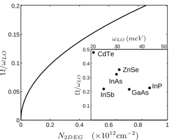
absorption in the conventional system of Zhu. Furthermore, this coupling strength is found little dependent on the electron density in the range of10~° cm~~, showing the secondary

Inspired by the injection locking technique used with optical lasers, we show that field emitted at frequency ω e from both non-degenerate modes a and b of the Josephson mixer can

(35) As the polariton annihilation operators are linear su- perpositions of annihilation and creation operators for the photon and the intersubband excitation modes, the ground state