HAL Id: hal-02988886
https://hal.archives-ouvertes.fr/hal-02988886
Submitted on 4 Nov 2020
HAL is a multi-disciplinary open access
archive for the deposit and dissemination of
sci-entific research documents, whether they are
pub-lished or not. The documents may come from
teaching and research institutions in France or
abroad, or from public or private research centers.
L’archive ouverte pluridisciplinaire HAL, est
destinée au dépôt et à la diffusion de documents
scientifiques de niveau recherche, publiés ou non,
émanant des établissements d’enseignement et de
recherche français ou étrangers, des laboratoires
publics ou privés.
Consensus modes, a robust description of protein
collective motions from multiple-minima normal mode
analysis-application to the HIV-1 protease
Paulo Batista, Charles Robert, Jean-Didier Maréchal, Meriam Hamida-Rebaï,
Pedro Pascutti, Paulo Bisch, David Perahia
To cite this version:
Paulo Batista, Charles Robert, Jean-Didier Maréchal, Meriam Hamida-Rebaï, Pedro Pascutti, et
al.. Consensus modes, a robust description of protein collective motions from multiple-minima normal
mode analysis-application to the HIV-1 protease. Physical Chemistry Chemical Physics, Royal Society
of Chemistry, 2010, 12 (12), pp.2850. �10.1039/b919148h�. �hal-02988886�
Consensus modes, a robust description of protein collective motions
from multiple-minima normal mode analysis—application to the HIV-1
protease
w
Paulo Ricardo Batista,
abCharles Herbert Robert,
bdJean-Didier Mare´chal,
cMeriam Ben Hamida-Rebaı¨,
bPedro Geraldo Pascutti,
aPaulo Mascarello Bisch
aand David Perahia*
bReceived 16th September 2009, Accepted 23rd December 2009 First published as an Advance Article on the web 1st February 2010 DOI: 10.1039/b919148h
Protein flexibility is essential for enzymatic function, ligand binding, and protein–protein or protein–nucleic acid interactions. Normal mode analysis has increasingly been shown to be well suited for studying such flexibility, as it can be used to identify favorable structural deformations that correspond to functional motions. However, normal modes are strictly relevant to a single structure, reflecting a particular minimum on a complex energy surface, and are thus susceptible to artifacts. We describe a new theoretical framework for determining ‘‘consensus’’ normal modes from a set of related structures, such as those issuing from a short molecular dynamics
simulation. This approach is more robust than standard normal mode analysis, and provides higher collectivity and symmetry properties. In an application to HIV-1 protease, the low-frequency consensus modes describe biologically relevant motions including flap opening and closing that can be used in interpreting structural changes accompanying the binding of widely differing inhibitors.
Introduction
The structural biology revolution has led to rapid growth in the number of known protein sequences and 3D structures,1,2
increasingly making clear the relationship between structure and function. But proteins are not static entities. They have to be flexible to interact with other molecules and perform their functions.3Even in crystal structures, significant flexibility can be inferred from values of the thermal B-factors,4,5 while
NMR structure determination results in families of dozens of structures, directly reflecting protein dynamics.6 This
dynamical aspect increasingly extends the dual concept of ‘‘structure and function’’ into the triplet structure/dynamics/ function.7–9
Complementing experimental methods for structure determination is the use of computational methods to investigate
dynamics, such as molecular dynamics (MD) simulations. MD calculations employ empirical force-fields and allow exploration of different regions of the vast conformational space, generating a trajectory reflecting macromolecular dynamics on different time scales.10–13 MD simulations have been successfully applied to describe diverse types of motions in different protein systems; e.g. active-site cleft opening/closing,14 peptide folding15 and ion-channel gating mechanisms.16
However, for large systems with precise representations (e.g. all-atom, explicit-solvent simulations) attainment of biologically interesting time scales can be prohibitively time consuming. Further, certain large-amplitude motions occur only rarely in MD simulations: some subunit, domain or loop motions take place on the millisecond time scale or longer.17–19
The correct description of such long-timescale motions thus remains a significant challenge.
Normal mode (NM) analysis is well suited for studying internal protein collective motions.20–25 It has proved especially useful for studying conformational changes since the observation that the lowest frequency modes compare well with crystallographically observed conformational changes.26–28Furthermore, such analyses can suggest motions of functional importance not yet observed in structural studies.29,30One advantage of NM analysis lies in its capturing
of the directions of lowest curvature of the potential energy surface, which correspond to large-scale internal motions of the protein. However, as with all methodologies, NM analysis has its own limitations.
One shortcoming of traditional NM analysis is its strict validity for small amplitude motions around a structure
aInstituto de Biofı´sica Carlos Chagas Filho, Universidade Federal do
Rio de Janeiro, 21941-902, Rio de Janeiro, Brasil
b
Institut de Biochimie et Biophysique Mole´culaire et Cellulaire, UMR8619, Universite´ Paris-Sud 11, 91405 Orsay, France. E-mail: [email protected]; Fax: +33-(0)1-69 85 37 15; Tel: +33-(0)1-69 15 63 20
cUnitat de Quı´mica Fı´sica, Departament de Quı´mica,
Universitat Auto`noma de Barcelona, Campus de Bellaterra, Cerdanyola del Valle`s, 08193, Catalonia, Spain
dLaboratoire de Biochimie The´orique, Institut de Biologie Physico
Chimique, 13 rue Pierre et Marie Curie, 75005 Paris, France w Electronic supplementary information (ESI) available: S1 Summary of equilibration procedure. S2 A list of the PDB identifiers (A) and the RMSD for the crystal (B) and NMR (C) structure data sets. S3 Pseudocode describing the routine used to calculate the CM from the QHM analysis of modes trajectory. See DOI: 10.1039/b919148h
localized in a particular minimum of the potential energy, while the potential energy surface of a protein contains a huge number of such minima. By considering a manageable number of minima around a given state, which represent ‘inherent structures’,31 it is in general possible to estimate
thermo-dynamic and kinetic properties of a protein.32–34 However,
vibrational analysis is often performed only for a single energy minimum, usually that corresponding to the energy-minimized crystal structure and taken to be representative, without formal acknowledgment of the fact that the true biological ‘‘structure’’ consists of an ensemble of closely related conformations. The significance and generality of NM pertaining to a given particular structure has thus been questioned.35
Nevertheless, several approaches have been taken to accommodate the multiple-minima nature of the potential energy surface. van Vlijmen and Karplus35 explicitly calculated NM for several energy-minimized protein structures sampled from MD simulations and compared them, and showed that by averaging certain properties calculated from the individual NM analyses, a better agreement with experimental and MD simulation results was obtained. Kitao and co-worker’s ‘‘jumping among minima’’ (JAM) model34 describes multiple energy basins (substates) separated by barriers that can nevertheless be crossed on the timescale of MD simulations. Protein conformational fluctuations are then decomposed in terms of intra- and inter-substate motions, the former well-described by NM analysis and the latter, including anharmonic movements, associated with the remaining fluctuations in the protein dynamic trajectories. Such approaches are very useful in better defining the behavior of a macromolecule using MD studies.
In this article we focus on synthesizing the harmonic information present in the multiple minima of the potential energy surface of a protein. We describe a new theoretical framework for defining normal modes consistently from a set of related structures, which we call ‘consensus modes’ (CM). The different structures correspond to different minimum energy points on the potential energy surface, obtained from MD sampling or from experimentally determined structures. A basic principle of the CM calculation is the assumption that the shape of the potential energy surface can be better exploited when multiple-minima topological information is considered. The use of multiple minima reduces bias caused by local features of the surface having relevance only to a particular minimum, as was highlighted by ref. 35. The atom fluctuations calculated by the CM can be directly compared to those obtained by averaging the results obtained in the individual NM determinations, but other features show novel properties. We show in particular that CM calculated over a set of structures issuing from an MD simulation furnish an improved description of protein internal motions, being able to provide more robust, statistically-representative directions of protein motions. Consensus modes provide a new way to study large-scale protein flexibility, and may have implications in protein folding and function including protein–protein and protein–ligand interactions (docking predictions).36
HIV-1 protease as an application system. We adopted here the apo form of the protease of HIV-1 to demonstrate
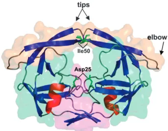
the CM approach. The aspartic HIV-1 protease (PR) functions as a homodimer (99 amino acids/chain) and plays a critical role in the HIV-1 life cycle;37,38it is considered one of the major targets of anti-AIDS drugs.39 PR can be divided into three principal regions (Fig. 1): the core domain, situated at the interface between the monomers and which contains the active site (the pair of catalytic triads Asp–Thr–Gly); the terminal domain containing both N and C terminals, which is important for dimerization; and the flap domain, which consists of two flexible hairpins at the entrance of the hydrophobic active-site cleft and which needs to open (close) to allow ligand entrance (stabilization).40
The flap domain is the most flexible region of PR, exhibiting major structural differences between the bound and free states,41,42 with transitions occurring on the ms–ms time scale.43,44
PR is an intensively studied protein, both experimentally and theoretically,45–51 with more than 270 solved
structures—NMR and crystallographic, unbound and complexed with different inhibitors—available in the PDB.2 These structures provide a rich source of data for comparison with computational results. For example, in a study of multiple PR structures from the PDB, Yang et al. showed close correspondence between the motions obtained from principal component analysis (PCA) and from a simplified NM approach (the elastic network model), suggesting that NM, even with a simplified potential, can explain the overall features of the structural differences arising from sequence variation and binding of different ligands.52
But a complete description of PR flexibility requires a correspondingly detailed description of the potential energy surface. The consensus modes approach allows one to better incorporate such detail from multiple, related PR structures while retaining the simplicity of a NM description.
Fig. 1 HIV-1 protease (PR) structure. Cartoon representation of PR colored by secondary structure: blue (b-sheets), red (a-helix) and gray (coil and loop). The solvent accessible surface (transparent) was colored in order to represent the principal PR domains: orange (flaps domain), light green (core domain) and magenta (dimerization domain—N and C terminals). The flap elbows, tips (Ile50), and catalytic residues (Asp25) are highlighted.
Theory
NM analysis is generally applied to a single structure that corresponds to a minimum in the 3N dimensional potential energy surface, N being the number of atoms of the system considered. In the neighborhood of this minimum, the surface is taken to be quadratic and is described by the Hessian matrix, F, whose elements are the second derivatives of the potential energy function with respect to the mass-weighted atomic coordinates (qi). Diagonalization of the Hessian then
provides the NM vectors and frequencies.22
At a given temperature, the Hessian, F, is related to the inverse of the covariance matrix of atomic displacements, r, by:
F = kBTr"1, (1)
where kB is the Boltzmann constant and T the absolute
temperature, and each element of r is defined as rij=hqi" hqiii
hqj" hqjii.53,54Each element of the covariance matrix within the
normal mode theory is given by:
sNM ij ¼ kBT X 3N"6 l¼1 ailajl o2 l ; ð2Þ
whereailis the ith component of the lth normal mode vector, and
olis the frequency of lth normal mode, and the sum is over the
3N" 6 internal normal modes.54
In the CM approach, the NM analysis is performed for each of a set of Ns different energy-minimized structures, taking
care that each structure has the same orientation (obtained by least-squares superposition). The different structures considered in the calculation of the CM in this study were obtained from MD simulation (see Experimental procedures). A new covariance matrix, sCM, is then defined as the mean
over the Nsindividual covariance matrices as defined above,
and expressed as: sCM ¼N1 s XNs s¼1 sNM s : ð3Þ
This matrix is termed the ‘consensus covariance matrix’. The influences of similar vibrational modes are reinforced in the averaging procedure, while local biases are reduced. The eigenvectors and eigenvalues of this matrix determine the consensus modes and their frequencies. The procedure is represented schematically in Fig. 2.
It should be pointed out that CM are distinct from quasi-harmonic modes (QHM) which are obtained directly from the mass-weighted covariance matrix calculated from MD trajectories.53–55The CM covariance matrix, however, is constructed using an analytical formulation of the shape of the energy surface in the region of each sampled minimum, while the QHM analysis uses only the sampled coordinates themselves. In particular, we note that QHM provide little information concerning timescales longer than that of the MD simulation itself.56 In contrast, the CM directly incorporate topological information about the potential energy surface, and can thus contain longer timescale information, albeit within potential energy wells.
Results and discussion
Experimental validation of MD from NMR data
MD simulations were carried out on the HIV apo-PR structure (PDB code 1 hhp)57in order to obtain the various conformations for NM analyses and subsequent CM determination. The system was extensively equilibrated so that the derived modes reflect the dynamics of structures belonging to a stable stationary stage of the simulation, thus reducing artifacts
Fig. 2 Schematic view of the consensus mode calculation for a series of sampled minima of the potential energy surface, each associated with a distinct normal mode description (different sets of colored arrows). The sum of covariance matrices calculated for the different minima corresponds to a superposition of their individual normal mode solutions, for which the corresponding motion is captured in the calculation of the consensus modes.
due to differences between the periodic water box (MD) and the crystal environments.58 We conducted this equilibration
procedure very carefully (as summarized in Fig. S1;w see details in Experimental procedures) to avoid problems in solvation, as discussed by Meagher et al.59 who have shown that poor solvent equilibration in the active site region leads to unexpected high amplitude fast flap motions (collapse/destabilization in a few hundred ps). We also verified that the number of water molecules within the active site was close to the number found in that study (data not shown). We also calculated the S2 N–H order parameters from the 10 ns of MD production, which showed very good agreement with NMR results45(Fig. 3). This confirms that our MD simulation
reproduced at least the sub-ns/ns dynamics of PR. Sampled conformations for CM calculations
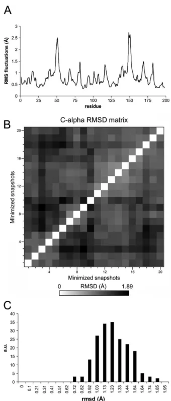
The structural variability of a protein in a stable state reflects the breadth of the corresponding free-energy minimum. The CM calculation allows such variability to be taken into account. In this study, structures were sampled every 50 ps throughout the initial 1 ns of the production MD simulation. This timescale was shown to be sufficient for convergence of the subspace including the so-called singly and multiply-hierarchical motions in the study of Kitao et al. for a protein of similar size.34 It is also possible that other sampling strategies could potentially be applied to better exploit different regions of the potential energy surface, e.g. a clustering analysis based on root mean square distance (RMSD) could initially be performed, or a larger sample set could be used. However, we found that the current procedure provided satisfactory results. The structural differences between sampled structure pairs, as measured by the Ca RMSD,
averaged 1.22 & 0.22 A˚ (Fig. 4B and C). This is somewhat larger than the variability seen in the PR crystal structures studied by Zoete et al.50but consistent with MD sampling in other systems (e.g. ref. 35). The Cafluctuations among the
20 minimized snapshots (Fig. 4A) followed the same pattern as seen in the literature for apo PR MD simulations:14,48,59high
deviations in the flap region (around residue 50/149) and small deviations in the active site (around residues 25/124). Consensus modes reflect the mean fluctuation behavior of the protein in the sampled minima
The Ca-fluctuations obtained with consensus modes and
those obtained by normal mode analysis of the individual
sampled structures are shown in Fig. 5. The CM fluctuations (bold black line) correspond to the average of the NM fluctuations as seen from eqn (3). The observed variability in the individual NM analyses arises from variations in atomic positions in the different sampled structures corresponding to different regions of the potential energy
Fig. 3 N–H S2 order parameter calculated from the 10 ns MD simulation compared to the experimental results from ref. 45.
Fig. 4 The structural variability of sampled structures used in the CM calculation. (A) Cafluctuations calculated from the 20
energy-minimized snapshots. (B) The Ca RMSD structural differences
between sample pairs. (C) Distribution of pairwise RMSD distances shown in (B).
surface. This effect clearly appears in the variety of individual NM fluctuation profiles (thin colored lines), which show peaks that are not present in the CM. Such extraneous peaks reflect fluctuations that are specific to a given particular structure but which have little effect on the average behavior of the molecule. CM has thus filtered out such unusual fluctuations, and this is one of the reasons for calling them ‘‘consensus modes’’.
The fluctuations obtained with our consensus approach are in good agreement with those obtained from crystallo-graphic B-factors (bold red line in Fig. 5), the Pearson correlation coefficient, R, between them being 0.69. It can also be noted that the CM fluctuations show high symmetry between the two chains (R = 0.87). This is in contrast with the results obtained from individual NM analysis fluctuation profiles, for which the interchain correlation was found to be 0.42& 0.1.
Consensus modes define a more complete conformational space for describing large amplitude motions
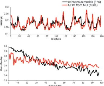
The full MD simulation was used to calculate the QHM, which are related to the principal components or the essential modes of the system. The atomic fluctuations from the 10 ns MD QHM presented in Fig. 6A are similar to those obtained from the CM. However, atom fluctuations alone provide only limited information when comparing two different sets of collective movements. In order to address how the large amplitude space described by the CM differs from that described by the QHM, we analyzed to what extent each of the QHM can be represented within the subspace defined by the 97 lowest-frequency CM, and vice versa, using a cumulative projection analysis (see Experimental procedures). Each of the first 20 lowest frequency QHM vectors derived from the 10 ns MD can be represented in the low-frequency CM vector space with a cumulative overlap (CO) greater than 0.8 (Fig. 6B, black line), with the first three lowest frequency vectors displaying CO values very close to 1. That is, the large-scale QHM movements are largely accounted for in the vector space spanned by the low-frequency CM. In contrast, the corresponding lowest-frequency CM movements are less well accounted for in the QHM space (red line in Fig. 6B). These results indicate that the low-frequency CM space is more complete than that of the QHM, despite the fact that the QHM were calculated from a simulation that was 10 times longer than the sampling period used for the CM calculation. As mentioned above, this is due to information present in the CM concerning the shape of the potential energy surface, which comes from the individual NM analyses used for their calculation.
Consensus modes from 1 ns MD present more collectivity than quasi-harmonic modes from 10 ns MD
Normal modes correspond to collective degrees of freedom, but a certain number of them can correspond to localized motions, whereas others can involve a large set of atoms moving together. We considered here a definition of the collectivity in terms of the breadth of the distribution of the
Fig. 5 Root mean square fluctuations (RMSF) calculated for Ca
atoms derived from the NM for each of the 20 MD snapshots (colored thin lines) and from the CM (bold black line). Also shown are the fluctuations derived from the normalized crystallographic temperature factors from the 1hhp crystal structure (bold red line). Protein residues are numbered from 1–99 for chain A and 100–198 for chain B.
Fig. 6 Correspondence between low frequency CM (1 ns) and QHM from 10 ns MD. (A) Comparison of CaRMSF derived from the CM
(black) and from the QHM calculated from 10 ns of MD (red). (B) Cumulative overlap of each QHM with the 97 lowest frequency CM (black) and of each CM with the 97 lowest frequency QHM (red). Modes are numbered in increasing frequency.
Fig. 7 Degree of collectivity of PR motions. The collectivity index,k, was calculated as described in Experimental procedures for each CM derived from the first ns of MD production (black) and for each QHM calculated from the full 10 ns MD (red). The mean collectivity along with the standard deviation over the NM of the 20 MD snapshots was also calculated (green). Modes are numbered in increasing frequency.
amplitudes of atom movements in a given mode. Collective (global) motions have been shown to be related to important biological conformational changes.25,29,60,61Fig. 7 shows that low frequency CM from the 1 ns MD simulation (black line) present higher collectivity than the corresponding QHM from the 10 ns simulation (red line). Further, in the CM, the high collectivity is concentrated in the lowest frequency modes, while in the QHM we see no dependence on the frequency. Interestingly, the mean NM collectivity values (green line), calculated over the same 20 MD snapshots, are significantly lower than those of the CM, although they are slightly larger than the QHM collectivities. Indeed, while the CM fluctuation profile can be seen from eqn (3) to be the average of the individual NM fluctuation profiles, there is no such simple relation to the individual NM collectivities. The higher collectivity is an additional property of the CM, which syn-thesize the characteristics of the different minima on the potential energy surface.
Versatility for computing consensus modes for different subsets of atoms
In the CM calculations, energy minimization and NM analysis are first performed for a series of structures, here protein-plus-water-layer systems issuing from molecular dynamics simulations. Thereafter, the mass-weighted consensus covariance matrix (rCM) can be calculated for any desired
subset of atoms (e.g. protein-only, backbone only, Ca, etc.),
and diagonalized, resulting in CM directions and frequencies for the considered selection of atoms. The results presented in the previous sections correspond to a reduction of the protein–water system to protein only, and thus they implicitly take into account the influence of the different water configurations. The CM frequencies calculated in this manner were slightly larger than those of the individual NM by a few cm"1due to the system reduction (data not shown).
In what follows, a further reduction is achieved, in which only the subset of Caatoms of our system is retained. We
will refer to the CM recalculated for the subset of Caatoms as
Ca-CM. The advantage of computing on Cais that redundant
motions of the backbone are eliminated. Such a reduction can also lead to better-averaged vectors integrating the mean effects of specific side-chain couplings with the backbone. This allows the filtering off of local motions and leads to a better representation of the global motions. Finally, using only Caatoms also permits the comparison of dynamics of proteins
of similar lengths but with different sequences, or of conserved domains in a protein family, making homology studies possible. We note that the CM approach can also be adapted to modes calculated from elastic network models on multiple structures.
Use of Ca-CM to compare theoretical and experimental motions
By reducing the protein representation to Ca atoms we used the consensus mode approach to identify collective motions inferred from X-ray and NMR structures of HIV-1 proteases with different sequences. We also performed principal component analysis (PCA) over these two different experimental datasets, as described in Experimental procedures.
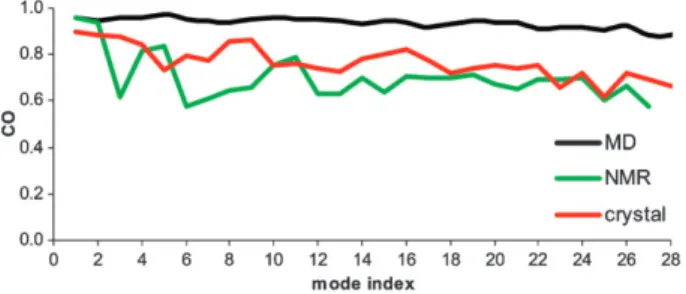
Fig. 8 shows the cumulative overlap values of the PCA components with the low frequency Ca-CM subspace. The
Ca-CM subspace describes to a large extent the PCA results
for both structural datasets, with cumulative overlap values ranging from 0.58 to 0.97. This figure also shows that the CO of the QHM, obtained from the 10 ns MD, in the Ca-CM
space was even higher (above 0.9). The latter comparison shows that the fundamental backbone movements are better represented using Ca-CM than all-atom CM, which gave CO
values between 0.75 and 0.90 for the same number of modes (Fig. 6B). This improvement is due to the averaging effect discussed above.
The values of the cumulative overlap of the 97 lowest-frequency Ca-CM with the PCA modes from the X-ray or
NMR PR datasets, although still high, are inferior to those of the QHM from the MD simulations. This is partly due to the fact that the experimental PR structures are almost all of the bound form, containing either inhibitors or substrates, and thus with the flaps in a closed conformation, while the MD simulations were performed starting with the unbound form of the protein, with flaps in a semi-open conformation.
Biological relevance of consensus mode analysis
Low-frequency/large-amplitude collective motions are important in describing long-timescale dynamics of proteins, consisting in many cases of domain motions that are related to biological function. One of the important aspects emerging from our results is that CM allow the characterization of more collective motions than can be obtained directly from longer MD simulations via quasiharmonic (or PCA) analysis or from individual NM determinations. In our analysis of PR using the CM, the lowest frequency modes are seen to be related to expansion or deformation of the active-site, including translational or rotational motions between the monomers and movements in the flap domains. As shown in Fig. 9, all these types of movements can be important for substrate or ligand binding. Such movements are only observed in very long MD simulations.44,49,62Flap dynamics
have been investigated by NMR showing that motions on two different timescales occur in the flap region of the free PR, one on the nanosecond45and the other on the micro to millisecond timescale,43 as suggested by a course-grained MD study of
apo PR system.44
Fig. 8 Cumulative overlap, in the subspace of the 97 lowest frequency Ca-CM, of the collective-movement vectors obtained by different
methods: QHM (black), X-ray PCA (red), and NMR PCA (green). In each case the results for the first 28 large-amplitude modes are shown. Modes are numbered by decreasing eigenvalue.
In both the Ca-CM and all-atom CM, the first two slow
modes are related to motions of translation/rotation between the monomers and may be implicated in the flexibility of each chain to allow enzyme accommodation after ligand binding. We also found two modes to be especially related to significant flap domain motions. The third lowest-frequency consensus mode describes flap opening and closing, while the fifth mode is related to variation of the distance between the tips of the flaps and the catalytic residues Asp 25, resulting in changes in active site shape and volume. The third lowest frequency CM is related to the intrinsic plasticity of the PR active site necessary for binding different ligands. To demonstrate this we chose two structures with representative differences in the active-site volume and inhibitor size: 4hvp and 1aid (Fig. 9A and B), as in ref. 6, in which the authors showed a concordance between the first collective mode of motion and the differences in the flap region between these two structures. The fifth lowest frequency Ca-CM describes a
movement in the direction of the conformational transition between the two different structures (Fig. 9A) with an overlap of 40% (see Experimental procedures) between the CM vector and the vector describing this conformational change.
(We note that the overlap would be significantly higher if the calculation took into account only the more limited region considered in the analyses of Zoete et al.50)
The third and fifth lowest-frequency CM describe flap opening and closing motions as well as structural changes occurring upon ligand binding, such as that observed in the conformational change between the open, apo-form (1HHP) and the closed conformation (4HVP), in which PR is bound to an inhibitor (Fig. 9C). Such motions are important for the entrance and stabilization of the ligand in the active site. Each of these two Ca-CM presents an overlap with the 4hvp to 1hhp conformational transition of around 30%. These directions of movement are presented in Fig. 9D. We also observed that motions of the flap tips are coupled to other domain motions, mainly in the flap elbows. This suggests that mutations or inhibitor binding in this region could potentially alter the dynamics of flap motions and interfere with the accessibility and interaction of ligands within the active site.
Conclusion
Predicting long-time dynamics of proteins is necessary to fully understanding their biological function. Molecular dynamics approaches can be used to describe the variety of conformations that a flexible protein can assume, but this technique can be expensive and inefficient for investigating large-scale motions, which may only appear at longer timescales (micro- to milliseconds). Interest has thus grown in exploiting alternative approaches such as all-atom NM or elastic normal mode (ENM) analyses (e.g. ref. 63) that make maximum use of a single protein structure. These approaches can provide estimates of the large-scale, collective motions of the protein. However, a statistical picture is missing, for, as we have seen, a given single structure may lead to dynamics results that are not representative of the overall behavior. The consensus modes approach we have described allows one to obtain collective macromolecular motions from a set of related protein structures, and is based on the curvature of the potential energy surface near each structure making use of normal mode theory. The consensus modes correspond to more robust descriptions of the large scale movements of a macromolecule than the normal modes obtained for a single structure. The CM is not limited to full atom NM calculations, but can also be adapted to ENM calculations on multiple structures. Consensus modes may also be useful to extend the JAM approach itself34 which was presented using only a single NM determination to model the intra-substate motions of the protein—the multiple minima information synthesized by the CM would improve the robustness of this approach.
Besides reducing potential artifacts, consensus modes also show more collectivity than either the normal modes of the individual structures or the quasi-harmonic modes obtained from an MD simulation ten times longer than that used in their calculation. Moreover, in the particular case of the homodimeric HIV-1 protease, the consensus modes display increased symmetry when compared to normal modes of the individual structures or to quasi-harmonic modes from MD simulations. The consensus mode approach may be applied to multiple X-ray or NMR structures in order to obtain the most
Fig. 9 Low-frequency CM movements in relation to the intrinsic flexibility of PR flaps. (A) The backbone trace of two structures of bound forms of PR, 4hvp (in blue) and 1aid (in red), as well as of intermediate structures described by the 5th lowest frequency CM. The intermediate structures were generated by displacing the mean structure in the& directions along the CM, up to an RMS of 0.6 A˚. (B) Mode describing the change of the shape and volume of the binding site of PR which appears necessary to accommodate ligands of various sizes. (C) Least-squares superposition of the backbone of bound (4hvp, in blue) and free PR (1hhp, in red). (D) Vectors (represented by arrows) of the 3rd and 5th lowest frequency CM involved in the flap motions that describe the conformational change from the closed (bound) to a semiopen (free) form. Cartoon arrows represent the overall directions of the motions of flap domains.
robust motions from them, and thus to provide a better description of global motions. They can allow the determination of key residues playing a role in motions that influence protein function or ligand-binding characteristics. Such information can then be exploited experimentally, for example in mutagenesis studies. Motions described by consensus modes may be further explored by using restrained energy minimization or MD simulation for a better structural and energetic descriptions of conformational changes.29,36,64Finally, we point out that the consensus mode approach allows a better treatment of hydration than can be attained in standard normal mode analysis, by implicitly taking into account different aqueous environments around the protein in the averaging process.
Experimental
MD simulations
The MD simulations were performed using NAMD 2.665with the CHARMM22 force field.66The homodimer structure of the apo-PR was solvated using a pre-equilibrated cubic TIP3 water box (approximately 55 000 atoms) with periodic boundary conditions. PME67 was used for electrostatic interactions with
non-bonded cutoffs of 12 A˚ for van der Waals and 10 A˚ for electrostatic interactions in the real space. We used SETTLE68and SHAKE69to fix water and protein bonds, respectively, allowing the use of an integration time of 2 fs, in the NPT ensemble.
The system was energy minimized using the conjugate-gradient algorithm, keeping the protein heavy atom positions harmonically restrained with a force constant of 50 kcal mol"1A˚"2 to avoid major structural changes. The restraint force constant was subsequently decreased to 5 kcal mol"1A˚"2during 72 ps
MD of the heating procedure, for which initial velocities were generated for a temperature of 20 K and the temperature slowly increased to 300 K using the Berendsen algorithm70
with a coupling constant of 0.67 ps. The output structure and final velocities were used to initiate the equilibration procedure with a coupling constant of 0.1 ps and at a pressure of 1 atm, with the position restraint force constant gradually decreased from 1 kcal mol"1 A˚"2 to zero over 1.5 ns. The equilibration was
carried out until the distances between the catalytic residue (Asp25) and the tip of the flap (Ile50) in both subunits were approximately equal, in order to have quasi-symmetrical behavior for the protein (3 ns). A production period of 10 ns was then carried out. (See the details and results in Fig. S1w). This trajectory was then reoriented using the same structure used for the CM calculation as reference, in order to avoid translation/rotation problems when comparing quasi-harmonic modes to CM vectors. Normal modes calculations
All-atom NM calculations were performed using the VIBRAN module of CHARMM71for 20 MD snapshot structures taken from the first nanosecond of production (every 50 ps), in order to calculate the consensus modes. The system consisted of the PR dimer plus the first layer of hydration.72This water layer helped avoid the collapse of the PR flaps during the minimization procedure. Water molecules whose oxygen was withinE4.0 A˚ of any protein atoms were included in the analyses, the precise cutoff being adjusted in order to have the same number of water molecules in each system (2790 atoms). Each system was minimized to a mean energy gradient of less than 10"5 Kcal mol"1 A˚"1. In order to have the same reference system for all the snapshots, normal modes were computed after having reoriented each minimized snapshot structure to a reference structure which was the energy minimized structure after the equilibration procedure. Consensus mode calculation
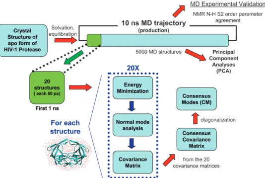
Fig. 10 shows a flowchart describing the CM approach from multiple minima NM calculations. The consensus covariance
matrix was established numerically in the following manner. The CHARMM program was used to generate harmonic trajectories for the normal modes related to the 20 different energy-minimized snapshot structures, but calculated with respect to the same, arbitrary reference structure. We considered here only the first 97 vibrational NM for each energy minimum. For each mode, the trajectory consisted of a complete single vibrational period containing 9 points. A single virtual trajectory for the desired subset of atoms was then created by concatenating the 20 ' 97 individual (harmonic) mode trajectories, and the consensus covariance matrix rCM generated. The eigenvalues and eigenvectors of
this matrix were then computed using the QUASI option in the VIBRAN module of CHARMM. Fig. S3w shows a pseudocode describing the routine used to calculate the CM from the QHM analysis of modes trajectory.
We emphasize that the individual structures comprising the concatenated trajectory thus consist of displacements of the (single) reference structure, but along the normal mode vectors calculated from the different minima. The resulting covariance matrix is thus exactly the same as that of eqn (3). (Indeed, the reference structure is recovered at the end of the procedure as the mean of the displaced structures.) This is quite different from the standard PCA or quasiharmonic mode calculation described in the following section, in which the structure displacements are heavily weighted by anharmonic motions.
Depending on the analysis, we computed the rCM for all
protein atoms (i.e. excluding water molecules) or for just the Ca atoms. Tests made using trajectories with more than 9
points in the vibrational period of each NM resulted in no significant improvement in the quality of the obtained modes. Quasi-harmonic mode calculations
The QHM were computed either for all the protein atoms (excluding the surrounding water molecules) or the Caatoms.
In the former case the Cartesian coordinates were scaled by the square root of the corresponding atomic masses. The covariance matrices of scaled coordinate changes were computed with over 5000 structures taken from the 10 ns production MD trajectory, the successive structures being separated by 2 ps time interval and superimposed on the average structure. These matrices were diagonalized to obtain the QHM by using the QUASI command of VIBRAN in CHARMM.
Overlap between CM and any other motion
The overlap between a given mode vector, Mi, and another
vector, X, is evaluated by their normalized projection, Oi(X) = MiX/JMiJJXJ, (4)
where Miis typically a consensus mode or normal mode vector
and X could be a mode vector from a different calculation, a quasi-harmonic or PCA mode vector, or a vector representing the conformational change between two different structures. A perfect match yields an overlap value of 1. We define the cumulative overlap between the first k lowest frequency modes and the vector X by:
(X, k) = (Si = 1,kO2i(X))
1
2, (5)
The cumulative overlap measures how well the space defined by a given set of modes (here we consider the k = 97 lowest-frequency modes) can include the motion indicated by the given vector X.
X-Ray and NMR data sets for principal component analysis All HIV protease structures used for this analysis were downloaded from the PDB and only the Cacoordinates were
considered. The NMR dataset comprised the 28 structures present in entry 1bve. The X-ray dataset contained 270 X-ray structures of PR, without missing residues. A list of the PDB identifiers (A) and the RMSD for each structure after superposition (B) are given in Fig. S2,w as well as for the NMR data set (C).
Degree of collectivity of a protein motion
The degree of collectivity of a protein motion can be expressed as the fraction of protein atoms participating significantly in the motion.26,73For a mode vector of length 3N with elements ai, this degree of collectivity,k, is defined as
k ¼N1exp "X 3N i¼1 a2 iloga 2 i ! ð6Þ
Ifk = 1, the conformational change is maximally collective, while ifk approaches 1/N, only one atom is involved in the conformational change.
Acknowledgements
CHR and DP wish to thank the Universite´ Paris-sud 11 Pluriformation Program DEMAIN and the IDRIS (Institut du De´veloppement et des Ressources en Informatique Scientifique) of the CNRS for access to resources used in performing the computations used for this work. PRB, PGP and PMB wish also to acknowledge the Brazilian agencies CNPq, CAPES and FAPERJ for financial support. JDM would like to thank the Sidaction foundation for support.
References
1 D. A. Benson, I. Karsch-Mizrachi, D. J. Lipman, J. Ostell and D. L. Wheeler, Nucleic Acids Res., 2007, 36, D25–30.
2 F. C. Bernstein, T. F. Koetzle, G. J. Williams, E. F. Meyer, Jr., M. D. Brice, J. R. Rodgers, O. Kennard, T. Shimanouchi and M. Tasumi, J. Mol. Biol., 1977, 112, 535–542.
3 R. Huber and W. S. Bennett, Jr., Biopolymers, 1983, 22, 261–279. 4 G. N. Phillips, Jr., Biophys. J., 1990, 57, 381–383.
5 W. C. Lu, C. Z. Wang, E. W. Yu and K. M. Ho, Proteins: Struct., Funct., Bioinf., 2006, 62, 152–158.
6 M. L. Teodoro, G. N. Phillips, Jr. and L. E. Kavraki, J. Comput. Biol., 2003, 10, 617–634.
7 A. Chollet and G. Turcatti, J. Comput.-Aided Mol. Des., 1999, 13, 209–219.
8 N. Sinha and S. J. Smith-Gill, Protein Pept. Lett., 2002, 9, 367–377. 9 L. K. Tamm, F. Abildgaard, A. Arora, H. Blad and
J. H. Bushweller, FEBS Lett., 2003, 555, 139–143. 10 M. Karplus and D. L. Weaver, Nature, 1976, 260, 404–406. 11 J. A. McCammon, B. R. Gelin and M. Karplus, Nature, 1977, 267,
585–590.
12 K. A. Henzler-Wildman, V. Thai, M. Lei, M. Ott, M. Wolf-Watz, T. Fenn, E. Pozharski, M. A. Wilson, G. A. Petsko, M. Karplus, C. G. Hubner and D. Kern, Nature, 2007, 450, 838–844.
13 K. A. Henzler-Wildman, M. Lei, V. Thai, S. J. Kerns, M. Karplus and D. Kern, Nature, 2007, 450, 913–916.
14 W. R. Scott and C. A. Schiffer, Structure, 2000, 8, 1259–1265. 15 E. Kim, S. Jang and Y. Pak, J. Chem. Phys., 2008, 128,
175104–175110.
16 W. Treptow, S. J. Marrink and M. Tarek, J. Phys. Chem. B, 2008, 112, 3277–3282.
17 H. Liu, S. G. Dastidar, H. Lei, W. Zhang, M. C. Lee and Y. Duan, Methods Mol. Biol., 2008, 443, 258–275.
18 L. A. Alcaraz, M. Del Alamo, M. G. Mateu and J. L. Neira, FEBS J., 2008, 275, 3299–3311.
19 G. C. Amorim, A. S. Pinheiro, L. E. Netto, A. P. Valente and F. C. Almeida, J. Biomol. NMR, 2007, 38, 99–104.
20 J. A. McCammon, B. R. Gelin, M. Karplus and P. G. Wolynes, Nature, 1976, 262, 325–326.
21 M. Levitt, C. Sander and P. S. Stern, J. Mol. Biol., 1985, 181, 423–447.
22 B. Brooks and M. Karplus, Proc. Natl. Acad. Sci. U. S. A., 1983, 80, 6571–6575.
23 D. Perahia and L. Mouawad, Comput. Chem., 1995, 19, 241–246. 24 E. Balog, J. C. Smith and D. Perahia, Phys. Chem. Chem. Phys.,
2006, 8, 5543–5548.
25 O. Keskin, S. R. Durell, I. Bahar, R. L. Jernigan and D. G. Covell, Biophys. J., 2002, 83, 663–680.
26 F. Tama and Y. H. Sanejouand, Protein Eng., Des. Sel., 2001, 14, 1–6.
27 L. Mouawad and D. Perahia, J. Mol. Biol., 1996, 258, 393–410. 28 P. Petrone and V. S. Pande, Biophys. J., 2006, 90, 1583–1593. 29 N. Floquet, P. Durand, B. Maigret, B. Badet, M. A. Badet-Denisot
and D. Perahia, J. Mol. Biol., 2009, 385, 653–664.
30 Z. Yang, P. Majek and I. Bahar, PLoS Comput. Biol., 2009, 5, e1000360.
31 N. Nakagawa and M. Peyrard, Proc. Natl. Acad. Sci. U. S. A., 2006, 103, 5279–5284.
32 D. J. Wales, Phys. Biol., 2005, 2, S86–93.
33 D. J. Wales and T. V. Bogdan, J. Phys. Chem. B, 2006, 110, 20765–20776.
34 A. Kitao, S. Hayward and N. Go, Proteins: Struct., Funct., Genet., 1998, 33, 496–517.
35 H. W. T. van Vlijmen and M. Karplus, J. Phys. Chem. B, 1999, 103, 3009–3021.
36 N. Floquet, J. D. Marechal, M. A. Badet-Denisot, C. H. Robert, M. Dauchez and D. Perahia, FEBS Lett., 2006, 580, 5130–5136. 37 M. A. Navia, P. M. Fitzgerald, B. M. McKeever, C. T. Leu,
J. C. Heimbach, W. K. Herber, I. S. Sigal, P. L. Darke and J. P. Springer, Nature, 1989, 337, 615–620.
38 N. E. Kohl, E. A. Emini, W. A. Schleif, L. J. Davis, J. C. Heimbach, R. A. Dixon, E. M. Scolnick and I. S. Sigal, Proc. Natl. Acad. Sci. U. S. A., 1988, 85, 4686–4690.
39 A. G. Tomasselli and R. L. Heinrikson, Biochim. Biophys. Acta, Protein Struct. Mol. Enzymol., 2000, 1477, 189–214.
40 A. Gustchina and I. T. Weber, FEBS Lett., 1990, 269, 269–272. 41 R. Lapatto, T. Blundell, A. Hemmings, J. Overington,
A. Wilderspin, S. Wood, J. R. Merson, P. J. Whittle, D. E. Danley and K. F. Geoghegan, et al., Nature, 1989, 342, 299–302.
42 A. Wlodawer and J. W. Erickson, Annu. Rev. Biochem., 1993, 62, 543–585.
43 R. Ishima, D. I. Freedberg, Y. X. Wang, J. M. Louis and D. A. Torchia, Structure, 1999, 7, 1047–1055.
44 V. Tozzini, J. Trylska, C. E. Chang and J. A. McCammon, J. Struct. Biol., 2007, 157, 606–615.
45 D. I. Freedberg, R. Ishima, J. Jacob, Y. X. Wang, I. Kustanovich, J. M. Louis and D. A. Torchia, Protein Sci., 2002, 11, 221–232. 46 E. Katoh, J. M. Louis, T. Yamazaki, A. M. Gronenborn,
D. A. Torchia and R. Ishima, Protein Sci., 2003, 12, 1376–1385. 47 R. Ishima and J. M. Louis, Proteins: Struct., Funct., Bioinf., 2008,
70, 1408–1415.
48 V. Hornak, A. Okur, R. C. Rizzo and C. Simmerling, Proc. Natl. Acad. Sci. U. S. A., 2006, 103, 915–920.
49 F. Ding, M. Layten and C. Simmerling, J. Am. Chem. Soc., 2008, 130, 7184–7185.
50 V. Zoete, O. Michielin and M. Karplus, J. Mol. Biol., 2002, 315, 21–52.
51 P. R. Batista, A. Wilter, E. H. Durham and P. G. Pascutti, Cell Biochem. Biophys., 2006, 44, 395–404.
52 L. Yang, G. Song, A. Carriquiry and R. L. Jernigan, Structure, 2008, 16, 321–330.
53 R. M. Levy, M. Karplus, J. Kushick and D. Perahia, Macro-molecules, 1984, 17, 1370–1374.
54 M. Karplus and J. N. Kushick, Macromolecules, 1981, 14, 325–332.
55 R. M. Levy, D. Perahia and M. Karplus, Proc. Natl. Acad. Sci. U. S. A., 1982, 79, 1346–1350.
56 M. A. Balsera, W. Wriggers, Y. Oono and K. Schulten, J. Phys. Chem., 1996, 100, 2567–2572.
57 S. Spinelli, Q. Z. Liu, P. M. Alzari, P. H. Hirel and R. J. Poljak, Biochimie, 1991, 73, 1391–1396.
58 J. Janin and F. Rodier, Proteins: Struct., Funct., Genet., 1995, 23, 580–587.
59 K. L. Meagher and H. A. Carlson, Proteins: Struct., Funct., Bioinf., 2005, 58, 119–125.
60 A. Thomas, M. J. Field and D. Perahia, J. Mol. Biol., 1996, 261, 490–506.
61 Q. Cui, G. Li, J. Ma and M. Karplus, J. Mol. Biol., 2004, 340, 345–372.
62 S. W. Rick, J. W. Erickson and S. K. Burt, Proteins: Struct., Funct., Genet., 1998, 32, 7–16.
63 M. M. Tirion, Phys. Rev. Lett., 1996, 77, 1905.
64 N. Floquet, S. Dedieu, L. Martiny, M. Dauchez and D. Perahia, Arch. Biochem. Biophys., 2008, 478, 103–109.
65 J. C. Phillips, R. Braun, W. Wang, J. Gumbart, E. Tajkhorshid, E. Villa, C. Chipot, R. D. Skeel, L. Kale and K. Schulten, J. Comput. Chem., 2005, 26, 1781–1802.
66 A. D. Mackerell, Jr, M. Feig and C. L. Brooks, 3rd, J. Comput. Chem., 2004, 25, 1400–1415.
67 U. Essmann, L. Perera, M. L. Berkowitz, T. Darden, H. Lee and L. G. Pedersen, J. Chem. Phys., 1995, 103, 8577–8593.
68 S. Miyamoto and P. A. Kollman, J. Comput. Chem., 1992, 13, 952–962.
69 J.-P. Ryckaert, G. Ciccotti and H. J. C. Berendsen, J. Comput. Phys., 1977, 23, 327–341.
70 H. J. C. Berendsen, J. P. M. Postma, W. F. Vangunsteren, A. Dinola and J. R. Haak, J. Chem. Phys., 1984, 81, 3684–3690. 71 Bernard R. Brooks, Robert E. Bruccoleri, Barry D. Olafson, David
J. States, S. Swaminathan and M. Karplus, J. Comput. Chem., 1983, 4, 187–217.
72 C. H. Robert, J. Cherfils, L. Mouawad and D. Perahia, J. Mol. Biol., 2004, 337, 969–983.