HAL Id: hal-00357048
https://hal.archives-ouvertes.fr/hal-00357048
Submitted on 29 Jan 2009
HAL is a multi-disciplinary open access
archive for the deposit and dissemination of
sci-entific research documents, whether they are
pub-lished or not. The documents may come from
teaching and research institutions in France or
abroad, or from public or private research centers.
L’archive ouverte pluridisciplinaire HAL, est
destinée au dépôt et à la diffusion de documents
scientifiques de niveau recherche, publiés ou non,
émanant des établissements d’enseignement et de
recherche français ou étrangers, des laboratoires
publics ou privés.
LITpro: a model fitting software for optical
interferometry
Isabelle Tallon-Bosc, Michel Tallon, Éric Thiébaut, Clémentine Béchet,
Guillaume Mella, Sylvain Lafrasse, O. Chesneau, Armando Domiciano de
Souza, G. Duvert, D. Mourard, et al.
To cite this version:
Isabelle Tallon-Bosc, Michel Tallon, Éric Thiébaut, Clémentine Béchet, Guillaume Mella, et al..
LIT-pro: a model fitting software for optical interferometry. Optical and Infrared Interferometry, Jun
2008, Marseille, France. pp.70131J-1, 70131J-9, �10.1117/12.788871�. �hal-00357048�
LITpro: a model fitting software for optical interferometry
I. Tallon-Bosc
a, M. Tallon
a, E. Thiébaut
a, C. Béchet
a, G. Mella
b, S. Lafrasse
b, O. Chesneau
c,
A. Domiciano de Souza
d, G. Duvert
b, D. Mourard
c, R. Petrov
d, M. Vannier
da
Université de Lyon, Lyon, F-69003, France ; Université Lyon 1, Observatoire de Lyon, 9 avenue
Charles André, Saint-Genis Laval, F-69230, France ; CNRS, UMR 5574, Centre de Recherche
Astrophysique de Lyon ; Ecole Normale Supérieure de Lyon, Lyon, F-69007, France
b
Laboratoire d’Astrophysique de Grenoble, CNRS, UMR 5571, F-38041 Grenoble, France
cUMR 6525 H. Fizeau, Univ. Nice Sophia Antipolis, CNRS, Observatoire de la Côte d’Azur, Av.
Copernic, F-06130 Grasse, France
d
UMR 6525 H. Fizeau, Univ. Nice Sophia Antipolis, CNRS, Observatoire de la Côte d’Azur, Parc
Valrose, F-06108 Nice cedex 2, France
ABSTRACT
LITpro is a software for fitting models on data obtained from various stellar optical interferometers, like the VLTI. As a baseline, for modeling the object, it provides a set of elementary geometrical and center-to-limb darkening functions, all combinable together. But it is also designed to make very easy the implementation of more specific models with their own parameters, to be able to use models closer to astrophysical considerations. So LITpro only requires the modeling functions to compute the Fourier transform of the object at given spatial frequencies, and wavelengths and time if needed. From this, LITpro computes all the necessary quantities as needed (e.g. visibilities, spectral energy distribution, partial derivatives of the model, map of the object model). The fitting engine, especially designed for this kind of optimization, is based on a modified Levenberg-Marquardt algorithm and has been successfully tested on real data in a prototype version. It includes a Trust Region Method, minimizing a heterogeneous non-linear and non-convex criterion and allows the user to set boundaries on free parameters. From a robust local minimization algorithm and a starting points strategy, a global optimization solution is effectively achieved. Tools have been developped to help users to find the global minimum. LITpro is also designed for performing fitting on heterogeneous data. It will be shown, on an example, how it fits simultaneously interferometric data and spectral energy distribution, with some benefits on the reliability of the solution and a better estimation of errors and correlations on the parameters. That is indeed necessary since present interferometric data are generally multi-wavelengths.
Keywords: optical interferometry, fitting software, data processing, Mira stars
1. INTRODUCTION
To fully exploit the scientific potential of existing interferometers, like the VLTI, astronomers have two types of data processing: image reconstruction and model fitting. Image reconstruction is applicable when interferometric measurements come from many different baselines, typically more than one hundred. This process relies on constraints (positivity, smoothness, etc.). The reconstructed image may be objective, but assumption may be made on a specific shape of the object too, like for example a radial symmetry.
Such a large number of measurements is not yet easily accessible in optical interferometry. When the number of measurements is sparse, i.e. for a poor uv-coverage, it becomes necessary to rely on assumptions on the shape of the object, with a limited number of free parameters: that is the domain of the model fitting.
Like image reconstruction, we may consider model fitting as an inverse problem, but with fewer degrees of freedom. We suppose that we know a direct model to compute simulated data from the parameters of a model of the object and if necessary, from a description of the interferometer during the observations. In the interferometric case, the model of data is complex and non-linear. Inverting means seeking a set of free parameters that allows us to fit the real data with the simulated ones: this is the function of the fitting process. It minimizes the distance between simulated and real data, the
Further author information: send correspondence to Isabelle Tallon-Bosc : [email protected]
!"#$%&'(&)*(+),-&-.*(+)#.-,.-/0.#-12(.*$#.*(31(4&-567(8%9:''.-2(;$''$&0(<=(>&)%9$2(?-&)@/$7.(>.'"'&)%5. A-/%=(/,(8A+B(C/'=(DEFG2(DEFGFH2(IJEEKL(M(EJDDNDKOPQEKQRFK(M(*/$S(FE=FFFDQFJ=DKKKDF
so-called residuals, by using an iterative process, and finally provides the values of the adjusted parameters with various useful informations like standard deviations of the parameters, their correlation and covariance matrices, confidence level, etc. Formally, those parameters maximize the likelihood, i.e. the probability of having observed the data given the current model. Since the covariances of the data are not estimated and stored in current data files,1 we assume that data are independent random gaussian variables. Thus maximizing the likelihood is equivalent to minimize a chi-square function which is the sum of Ndsquared weighted residuals, ri, where Ndis the number of data and the weighting is related to the standard deviation of the data, σi:
χ2(p) = Nd ! i=1 " ri(p) σi #2 . (1)
The residuals are generally computed as a difference between real and simulated data values, ri(p) = di− mi(p), but other expressions may be used, mainly for the phase of complex interferometric data.2 The main difficulty of model fitting is precisely the minimization of χ2(p), a non-convex criterion that exhibits many local minima in the space of parameters, p.
LITpro, for "Lyon Interferometric Tool prototype", is a model fitting software among others. Its particularity is to be designed to allow easy use and enrichment, in order to be useful both to astronomers with no particular expertise in optical interferometry and to more advanced users for more pioneering work. Thus, LITpro aims both to make the most of available facilities and, for instance to study new methods for leading the user to the best global minimum. Conceived and developed up-to-now in Lyon and implemented in Yorick∗, it is now tested by a group within the JMMC† research group, until its first public release by the end of this year. A powerful Graphic User Interface (GUI) in JAVA is also under development at Grenoble Observatory.
LITpro has been already described.3 So, we just recall in Section 2 its main features. In Section 3, we show how the software is able to fit simultaneously interferometric data and spectral energy distribution (SED), using a specific chromatic model function.4
2. DESCRIPTION OF LITPRO
2.1 Main Requirements
Essentially two main requirements have driven the design of LITpro.
The first request was to build a very flexible tool meeting opposite needs, i.e. both accessible to astronomers with no particular expertise in optical interferometry, but still useful for experts who wanted to address specific problems or to experiment new ideas. As a consequence, LITpro has an "expert" layer built upon a high level language, Yorick, to allow easy modifications and adds in the software. However, for a better accessibility, a GUI exposes parts of the functionalities in a simple way for the "non-expert" user. This combination allows the GUI to benefit from new possibilities once they are validated in the "expert" layer. So LITpro is by definition continuously evolving and is a place to gather and share experiences from various users.
The second request was to make the implementation of new models of objects as simple as possible. So the only needed output of the modeling functions is the Fourier Transform of the brightness distribution of the object at given coordinates (spatial frequencies, wavelengths and time). For example, to make the implementation of new modeling functions even simpler, coordinates or parameters are recognized by their names, so they can be given in any order in the list of arguments. The software computes all the necessary quantities (e.g. simulated data, images, SED) only from the returned Fourier Transform.
These requirements have implications in the different parts of the software that we summarize in the next sections.
∗Yorick is a free cross-platform data processing language written by D. Munro and available at http://sourceforge.net/projects/yorick/. †The web-site of the Jean-Marie Mariotti Center is http://www.jmmc.fr
2.2 Data Fitting
Architecture of the code allows various fitting algorithms to be implemented and selected, at least for experimenting new algorithms. Indeed, reliable and efficient ways to find the global minimum among numerous local minima is one major difficulty of non-linear model fitting and deserves more studies.
Currently, our workhorse of the fitting process is a Levenberg-Marquardt algorithm5 combined with a Trust Region method.6 The current algorithm was improved to account for bounds on the parameters and to automatically compute partial derivatives of the model by finite differences, since the user is not requested to provide any function for their computation.
At the end of the procedure, final reduced chi-square (i.e. chi-square divided by the number of degrees of freedom), standard deviations, covariance and correlation matrices allow the user to evaluate the reliability of his model. With the information given by the matrices, he can assess cross-dependencies between the parameters. Degenerate parameters are automatically detected and signaled to the user.
Some parameters may be degenerated, i.e. their values cannot been determined from the data. For example, this is the case with the total energy of the object when combining several elementary functions as a weighted sum, or when the total energy of a more elaborated model depends on a complex combination of several heterogeneous parameters. In such a case, the standard deviations of these parameters cannot be determined. This problem may be complex to solve by an action on the parameters, in particular for chromatic models. When this problem appears, we solve it by constraining the total energy to unity by the addition of a residual in the expression of χ2(Eq. (1)):
χ2!(p) = χ2(p) + Nd $ % j∆λjm(λj) % j∆λj − 1 &2 , (2)
where the sums are over all the bandwidths ∆λj, Ndis the number of data, and m(λj) is the value of the Fourier transform of the object at the zero spatial frequency (which is equal to the total flux) in each bandwidth. When the total energy is undetermined with the data, this additional term is zero, and the value of the χ2is unchanged.
2.3 Data Format
LITpro reads the data stored in the OI Exchange Format1 (OI-FITS). OI-FITS currently store interferometric data as squared visibilities (VIS2), amplitude and phase of complex visibility (VISAMP and VISPHI), amplitude and phase of bispectrum (T3AMP and T3PHI), and the corresponding errors on these quantities. LITpro re-organizes the arrays in memory, possibly after merging the data from various files, in order to simplify and speed up the forthcoming processes.
OI-FITS is now widely used in Optical stellar Interferometry but is yet limited. In particular, we need to store other quantities already measured by existing interferometers, like spectral energy distribution (SED),7, 8 or polarimetric data.7 Also, for complex visibility data, the format does not specify how these quantities have been estimated. For instance, they could be estimated from phase-referenced observations,9or from cross-spectrum between two spectral channels, one beeing considered as a reference. In this latter case, the reference spectral channel can be defined in different ways.8, 10 The knowledge of these specificities is necessary to correctly compute the simulated data when fitting.
In order to read this kind of data, LITpro now provides functions to easily import various format of data. This feature has been used for the example presented in Sec. 3.
2.4 Modeling of the object
LITpro offers elementary geometric models for the object as a library of classical functions (disc, ring, gaussian, center-to-limb darkening profiles, circular or elongated into one direction, etc) that can be combined to build up more complex shapes. The user can also easily implement its own functions.
Before launching the fit, modeling functions are linked to data files in a so-called modeling file. This can be done by filling directly this file as a form or through the GUI (see after). Several of such associations can be defined in the same modeling file in order to be fitted simultaneously. This is an asset to handle heterogeneous data like visibilities and SED, or to fit simultaneously a scientific target and its calibrator when working on raw visibilities. This latter example may be necessary to avoid the correlations introduced by the calibration of visibilities,11 which is in contradiction with the basic assumption of statistically independent measurements.
Through the modeling file, the actual parameters are named and associated to the arguments of the modeling functions. This is a means to use the same parameter in different functions. The user also sets the initial values of the parameters and their bounds if any, and selects the types of data to be fitted: VIS2, VISAMP, VISPHI, T3AMP, T3PHI, SED, etc.
2.5 Analysis Tools
Analysis of the results is a topic by itself and needs continuous improvements to display useful informations to the user. Currently, LITpro provides graphical tools for the user to visualize data, models, residuals, cuts in the χ2space, etc (see Sec. 3).
A function is provided to compute the image maps from the model of the object that only outputs the Fourier transform of the object, with the proper scale and sampling.
2.6 Graphical User Interface (GUI)
Since LITpro is a Yorick software, it first requires a multi-step installation process. Once installation is done, it also requires the user to write some Yorick code to configure each of its fitting processes. The command lines are simple, as showed at the VLTI school in Goutelas,3 but the user needs to know Yorick language basics and LITpro Application Programming Interface (API) if he/she wants to use LITpro comprehensively. So the need of building a GUI to offer LITpro as a desktop application became obvious: easy to install, easy to use, and hence accessible by a larger community, however with limited capabilities.
To create this desktop application, the Java platform has been chosen because it eases the creation of portable, net-worked, graphical user interfaces. Furthermore, lots of specialized libraries are available for Java, especially in the astro-nomical field. If applicable, our application tries to implement standards of virtual observatory and cross-operates with compatibles applications to broaden capabilities. It shares also some code and functionalities (such as feedback report, user help, etc) with the other Java graphical applications of the JMMC.
To provide specific model-fitting computation inside the Java GUI, the scientific code is not rewritten in Java but is delegated to the existing LITpro "expert" layer. This layer has been indeed deployed on a dedicated server, to provide Model-Fitting capabilities through a webservice across the Internet. Internally, LITpro uses a hierarchical dynamic struc-ture to store data, and model descriptions. The data format for ensuring the communication between the server and the GUI is based on Extensible Markup Language (XML). This is a natural way to store hierarchical information and is well supported under Java.
The GUI presents this XML hierarchy to the user through a main "tree" widget. The selection of any tree element shows a dedicated panel that displays details about the selected element. Each panel also drives user inputs by performing some verifications or automations. In addition to graphical help, the GUI also embeds interactive information items. Most of them are dynamically collected by querying the webservice. LITpro is able to expose its capabilities (such as the list of the object models available in its library for example) with their documentation or parameters constraints.
Once the user configuration is done thanks to all those mechanisms, the XML configuration file is transmitted to LITpro webservice. The server processes it through transformations of the Extensible Stylesheet Language (XSL) and automatically generates the Yorick code needed by LITpro as input batch files. The fit is then launched with the generated code, and the result is given back to the GUI for result browsing.
All those mechanisms allowed us to conveniently interface with the existing LITpro "expert" layer, without having to change any code. The only additional operation has been to write a function to transform LITpro internal data structure as XML files.
3. EXAMPLE OF A FIT ON HETEROGENEOUS DATA
The aim of this section is to present an example of a fit of a chromatic model on both multi-wavelength interferometric data and photometric data. For testing this LITpro capability, we have chosen to use IOTA data on RLeo, published by Perrin et al.,4mainly because fitting these data has been found not so easy.
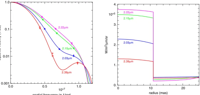
2.03µm 2.15µm 2.22µm 2.39µm 0.0 0.5 1.0 10+7 0.001 0.01 0.1 1.0
spatial frequency in 1/rad
squared visibility (VIS2)
2.03µm 2.15µm 2.22µm 2.39µm 0 10 20 0. 1. 2. 3. 4. 10+5 radius (mas) W/m 2/µ m/sr
Figure 1. Result of the fit of IOTA data obtained by Perrin et al.4 In log scale on the left, data are shown as crosses with (small) error
bars, and corresponding modeled data appear as circles, in the 4 sub-bands of the K band. On the right, the corresponding center-to-limb variations in each sub-bands show the star of radius 11 mas surrounded by the layer of radius 25 mas.
3.1 Modeling Function
We consider that a model is chromatic when the value of at least one parameter modifies the simulated data at all wave-lengths. This is the case for the model of a star surrounded by a thin molecular layer proposed by Perrin et al.4 The expression of the specific intensity of this model is:
I0(λ, θ) = B(λ, T!) exp " −τ(λ) cos θ # + B(λ, TL) '
1 − exp"−τ(λ)cos θ #(, if sin θ ≤ R!/RL, I0(λ, θ) = B(λ, TL)
'
1 − exp"−2τ(λ)cos θ #(, otherwise,
(3)
where B(λ, T ) is the Planck function at wavelength λ and temperature T , θ is the angle, at the layer surface, between the radius of the layer and the line of sight (|θ| < π/2), τ(λ) is the optical depth of the layer, R!, T! and RL, TL, are the radii and the temperatures of the star and the layer respectively. This spherical symmetric model results from an analytical solution of the radiative transfer calculations that is possible for this simplified configuration where a thin shell is separated by an empty space from the star.
The Fourier transform of I0(λ, θ) required by LITpro is computed by the Hankel transform of this circular symmetric brightness distribution. The model has 4 parameters (R!, T!, RL, TL), plus as many optical depths τias spectral channels centered on effective wavelength λi. With this model, changing T! or TL changes the shape of the object from one wavelength to another.
3.2 Perrin et al. Approach for RLeo
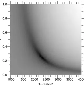
The interferometric data are squared visibilities obtained at the IOTA interferometer in 4 narrow sub-bands of the K band, centered at 2.03, 2.15, 2.22, and 2.39µm, plotted on Fig. 1. The main difficulty for fitting these data is due to the coupling of the temperatures of the star and the layer, because the interferometric data do not constrain the total flux of the model. This is apparent on the χ2cut along T
!and TL directions plotted on Fig. 2 when only the interferometric data are considered. This means that acceptable solutions could be found by setting one temperature to any arbitrary value in a large range.
The procedure reported by Perrin et al.4 for the determination of the parameters is as follows. They first sampled R ! and RLon a 2D grid and, for each fixed values (R!, RL) on the grid, they fitted all the other parameters starting from the
2000 2500 3000 3500 4000 4500 5000 1000 1200 1400 1600 1800 2000 T∗ (Kelvin) TL (Kelvin)
Figure 2. 2D cut in the χ2space (in log scale) along T !
(ab-scissa) and TL(ordinate) directions. The other parameters are
set to the solution found by Perrin et al.4 The map shows the
coupling of the temperatures when only the interferometric data are considered.
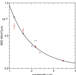
1 2 3 4 0.0 0.5 1.0 10−8 wavelength (µm) SED (W/m 2/µ m)
Figure 3. Comparison of a synthetic spectrum (continuous line) with photometric data12in J, H, K and L bands (crosses).
Squares are the fluxes computed with the actual values of the optical depths fitted in the 4 sub-bands in the K band, while the synthetic spectrum is computed from the parameters fit-ted to the interferometric data when assuming a layer optical depth of 1 at any wavelength.
somehow arbitrary values T!= 3000K, TL= 2000K, τ2.03 = 0.1, τ2.15= 0.5, τ2.22= 0.5, and τ2.39= 0.1 (see Eq. (3)). Then, the values of R!and RLwere determined from the minimum in this χ2grid.
In a second step, a similar approach aimed at the determination of the temperatures for the found radii, now fixed. T!and TLwere sampled on a 2D grid, and the optical depths were fitted for each fixed values (T!, TL) on this grid. At this step, the χ2function for the optical depths only, appeared close to convex and led to a fast convergence towards the optimum optical depths. But the obtained map was similar to the one on Fig. 2, showing a trough which does not allow a unique determination of the temperatures.
The solution came from applying a photometric constraint. A synthetic K magnitude was determine for each (T!, TL) in the χ2map, and the intersection of the temperature trough (see Fig. 2) and of the photometry-compliant area yield the best set of temperatures and their uncertainties. The values of the parameters for this solution are summarized in Table 1.
A synthetic spectrum computed from the parameters fitted on the interferometric data was successfully compared to photometric data established from the measurements of Whitelock et al.12 in J, H, K and L bands, after the K band was used to determine the temperatures. The same comparison is shown on Fig. 3. The synthetic spectrum (continuous line) is computed from the parameters fitted to the interferometric data when assuming a layer optical depth of 1 at any wavelength. It is not the place here to discuss the validity of this gross simplication, nor to justify the presented modeling on an astrophysical point of view. Our aim is only to evaluate the fitting procedures themselves. On the same graph, we have also plotted (squares) the flux computed with the actual values of the optical depths fitted in the 4 K sub-bands.
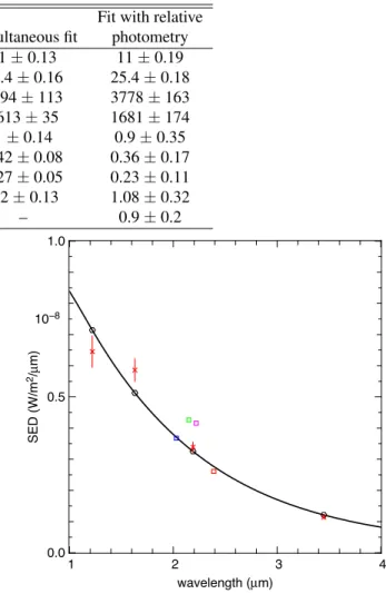
3.3 Simultaneous Fit on Photometric Data
The previous fitting procedure is hardly accessible to a "non-expert" user. With LITpro, we have tested the approach to fit all the parameters together, on interferometric and photometric data simultaneously. The aim is to benefit at most from all the constraints, particularly on the temperatures. Also, this approach allows an homogeneous estimation of the standard deviations of the parameters, and to compute their full correlation matrix.
The procedure for fitting is also easier and somehow simplified as follows. The first step is to get a first estimation of the size of the object by fitting a uniform disk on the interferometric data alone. We found a radius of 18.15 ± 0.03
Table 1. Summary of the values of the parameters found for the different approaches: original values from Perrin et al.,4solution found
with LITpro when fitting all the parameters altogether, and the same, but with relative photometry.
Fit with relative Parameter Perrin et al. Simultaneous fit photometry
R!(mas) 10.94 ± 0.85 11 ± 0.13 11 ± 0.19 RL(mas) 25.00 ± 0.17 25.4 ± 0.16 25.4 ± 0.18 T!(K) 3856 ± 119 3694 ± 113 3778 ± 163 TL(K) 1598 ± 24 1613 ± 35 1681 ± 174 τ2.03 1.19 ± 0.01 1 ± 0.14 0.9 ± 0.35 τ2.15 0.51 ± 0.01 0.42 ± 0.08 0.36 ± 0.17 τ2.22 0.33 ± 0.01 0.27 ± 0.05 0.23 ± 0.11 τ2.39 1.37 ± 0.01 1.2 ± 0.13 1.08 ± 0.32 γ – – 0.9 ± 0.2 2000 2500 3000 3500 4000 4500 5000 1000 1200 1400 1600 1800 2000 T∗ (Kelvin) TL (Kelvin)
Figure 4. 2D cut in the χ2 space (in log scale) along T !
(abscissa) and TL(ordinate) directions, when the other
pa-rameters are set to their final values of the simultaneous fit. Contrary to Fig. 2, the temperatures now can be determined, thanks to the constraints brought by the photometric data.
1 2 3 4 0.0 0.5 1.0 10−8 wavelength (µm) SED (W/m 2/µ m)
Figure 5. Same as Fig. 3, but after the simultaneous fit. Taking J and H measurements into account has lessen the SED at these wavelengths.
mas, to be used as a starting value afterward. We can notice that this value is almost twice the final value of R!(Table 1) obtained with the full chromatic model (Eq. (3)). In the second step, we estimate the temperature of this 18 mas uniform disk considered as a blackbody by a fit on the photometric data alone. This yields T! = 1540 ± 11K. Finally, we fit all the data with all the parameters, setting the model as a uniform disk with the previously found radius and temperature as a first guess. Thus, the initial value of the parameters are R! = 18 mas, T!= TL = 1540K, all optical depths to zero. RL is indifferent at this step and was set arbitrarily to 2R!. We have noticed that a successfull fit is achieved as long as the starting value of the temperature is chosen between 1000K and 4000K or as long as the initial value of RLis between 25 and 72 mas.
The final values of the parameters are shown in the Table 1. They only slightly differ from the values of Perrin et al. We can notice that the estimation of the standard deviations of the optical depths seems to be now more realistic.
Figure 4 shows from a χ2 cut along T
! and TL directions, that a minimum allows the temperatures to be directly determined at the opposite of the previous case (Fig. 2). The slight modification of the temperatures (T!is lower and TLis higher) is driven by the fit of the photometric data in the J and H bands (Table 1).
1000 1500 2000 2500 3000 3500 4000 0.0 0.2 0.4 0.6 0.8 1.0 T∗ (Kelvin) γ
Figure 6. 2D cut in the χ2space (log scale) along T
!(abscissa) and γ (ordinate) directions, when the diameter of the star is fixed to 18
mas, the value resulting from the fit of the interferometric data with a uniform disk. The map shows that the same unique minimum is reached from any starting values of the fitted parameters (γ, T!) on photometric data. The solution of this fit is then used as an initial
guess for fitting the full model (Eq. (4)) on both interferometric and photometric data.
3.4 Fit with Relative Photometry
Nowadays, interferometric data come with spectral information, for instance when dispersed fringes mode is used.7, 8 Simultaneous spectral information is an asset for many observed objects, but in this case, the photometry may be not calibrated and we can only rely on spectral features, like some particular lines for instance. We refer to this situation as relative photometry, since we can only compare flux between different spectral channels.
As a comparison with the previous case we will assume in this section that we have lost the calibration of the photometry in the previous data, only retaining the magnitude differences between J, H, K and L bands. We want to assess, in our particular case, how the previously fit is modified.
This case is simply achieved by adding a scaling factor γ in the previous chromatic model (Eq. (3)):
I(λ, θ) = γ I0(λ, θ). (4) With this model, χ2on interferometric data is not sensitive to γ which will be only determined by the average level of the flux in the photometric data, thus the temperatures will be only sensitive to the slope of the spectrum (see Fig. 5).
As in the previous case, fitting a uniform disk on the interferometric data alone gives an initial guess of 18 mas for the size of the object. Then, we consider again this disk as a blackbody and fit both its temperature T!and the scaling factor γ. This fit yields a unique solution γ = 0.25 ± 0.02, T!= 2339 ± 67K, for a wide range of starting values, because the χ2 space has a single minimum as shown on Fig. 6. These two fits allow us to easily get an idea of the size and the temperature of the object. As in the previous case, the general fit is then started with the full model configured as a uniform disk with these found parameters: R!= 18 mas, T!= TL= 2339K, γ = 0.25 and all optical depths set to zero.
The result shown in Table 1 is similar to the one obtained with absolute photometry, with only slightly larger standard deviations on the parameters.
4. CONCLUSION
We have described through a practical example the current capabilities of LITpro. The study of the fit on interferometric and photometric data on Rleo has pointed to the advantages of such a simultaneous fit of heterogeneous data. When such
data are not available, it appears essential that the SED becomes accessible within the OIFITS standard in order to allow fitting with relative photometry.
LITpro will continue to be improved. The current version of the Java GUI is still under development too. As both sides of the whole Model Fitting software are separated with a simple interface between them, development is conveniently done by two different groups of people within the Model Fitting team. The scientific group leverages its expertise in the field by working on the fitting-engine side (easily updatable on the server), while the technical group is in charge of all graphical interface developments. A first public release is foreseen by the end of 2008.
There are various directions of research we would like to go with LITpro. One of those is the search for global minimum of χ2to solve the critical problem of multiple minima. Another priority is to associate model fitting with the image reconstruction. When the latter is possible, it indeed may be still necessary to rely on model fitting for getting measurements and error bars on a few specific parameters of the object: that is possible with model fitting but difficult to obtain from a reconstructed image. So, still for a while, model fitting and image reconstruction are complementary tools for processing interferometric data and both are in full development.
ACKNOWLEDGMENTS
The software presented in this article has been implemented in Yorick, a free data processing language written by D. Munro (http://sourceforge.net/projects/yorick/).
REFERENCES
[1] Pauls, T. A., Young, J. S., Cotton, W. D., and Monnier, J. D., “Data exchange standard for optical (visible/IR) interferometry,” Publ. Astron. Soc. Pac.117(837), 1255–1262 (2005).
[2] Haniff, C. A., “Least-squares Fourier phase estimation from the modulo 2π bispectrum phase,” J. Opt. Soc. Am. A8(3232), 134–140 (1991).
[3] Tallon-Bosc, I., Tallon, M., Thiébaut, E., and Béchet, C., “Model fitting tutorial,” New Astron. Rev.51(8-9), 697–705 (2007).
[4] Perrin, G., Ridgway, S. T., Mennesson, B., Cotton, W. D., Woillez, J., Verhoelst, T., Schuller, P., Coudé du Foresto, V., Traub, W. A., Millan-Gabet, R., and Lacasse, M. G., “Unveiling Mira stars behind the molecules. Confirmation of the molecular layer model with narrow band near-infrared interferometry,” Astron. Astrophys. 426(1), 279–296 (2004).
[5] Dennis, J. E. and Schnabel, R. B., [Numerical Methods for Unconstrained Optimization and Nonlinear Equations], Prentice-Hall, Englewood Cliffs, NJ (1983).
[6] Moré, J. J. and Sorensen, D. C., “Computing a trust region step,” SIAM J. Sci. Stat. Comput.4(3), 553–572 (1983). [7] Mourard, D., Perraut, K., Bonneau, D., Clausse, J.-M., Stee, P., Tallon-Bosc, I., Kervella, P., Hugues, Y., Marcotto,
A., Blazit, A., Chesneau, O., Domiciano de Souza, A., Foy, R., Hénault, F., Merlin, G., Roussel, A., Tallon, M., Thiébaut, E., McAlister, H. A., Brummelaar, T. A. t., Sturmann, J., Sturmann, L., Turner, N. H., Farrington, C. D., and Goldfinger, P. J., “VEGA/CHARA: a new visible spectrograph and polarimeter on the CHARA array,” in [Optical and Infrared Interferometry], Schöller, M., Danchi, W. C., and Delplancke, F., eds., SPIE7013, paper 7013–74 (2008). [8] Petrov, R. G., Malbet, F., Weigelt, G., and et al., “AMBER, the near-infrared spectro-interferometric three telescopes
VLTI instrument,” Astron. Astrophys.464(1), 1–12 (2007).
[9] Quirrenbach, A., Mozurkewich, D., Buscher, D. F., Hummel, C. A., and Armstrong, J. T., “Phase-referenced visibility averaging in optical long-baseline interferometry,” Astron. Astrophys.286, 1019 (1994).
[10] Berio, P., Mourard, D., Bonneau, D., Chesneau, O., Stee, P., Thureau, N., Vakili, F., and Borgnino, J., “Spectrally resolved Michelson stellar interferometry. I. Exact formalism in the multispeckle mode,” J. Opt. Soc. Am. A16(4), 872–881 (1999).
[11] Perrin, G., “The calibration of interferometric visibilities obtained with single-mode optical interferometers - Com-putation of error bars and correlations,” Astron. Astrophys.400(3), 1173–1181 (2003).
[12] Whitelock, P., Marang, F., and Feast, M., “Infrared colours for Mira-like long-period variables found in the Hipparcos Catalogue,” Mon. Not. R. Astr. Soc.319(3), 728–758 (2000).