HAL Id: halshs-00497453
https://halshs.archives-ouvertes.fr/halshs-00497453
Submitted on 5 Jul 2010
HAL is a multi-disciplinary open access archive for the deposit and dissemination of sci-entific research documents, whether they are pub-lished or not. The documents may come from teaching and research institutions in France or abroad, or from public or private research centers.
L’archive ouverte pluridisciplinaire HAL, est destinée au dépôt et à la diffusion de documents scientifiques de niveau recherche, publiés ou non, émanant des établissements d’enseignement et de recherche français ou étrangers, des laboratoires publics ou privés.
What are Households Willing to Pay for Better Tap
Water Quality ? A Cross-Country Valuation Study
Olivier Beaumais, Anne Briand, Katrin Millock, Céline Nauges
To cite this version:
Olivier Beaumais, Anne Briand, Katrin Millock, Céline Nauges. What are Households Willing to Pay for Better Tap Water Quality ? A Cross-Country Valuation Study. 2010. �halshs-00497453�
Documents de Travail du
Centre d’Economie de la Sorbonne
What are Households Willing to Pay for Better Tap Water Quality ? A Cross-Country Valuation Study
Olivier BEAUMAIS, Anne BRIAND, Katrin MILLOCK, Céline NAUGES 2010.51
What are Households Willing to Pay for Better Tap Water Quality?
A Cross-Country Valuation Study
Olivier Beaumais CARE, University of Rouen
Anne Briand
CARE, University of Rouen
Katrin Millock
Paris School of Economics, CNRS
Céline Nauges
What are Households Willing to Pay for Better Tap Water Quality?
A Cross-Country Valuation Study
Résumé
Nous estimons la disponibilité à payer pour la qualité de l’eau du robinet sur des données d’enquête de 10 pays de l’OCDE. Nos résultats indiquent que les ménages sont prêts à accepter une augmentation de 7,5% de leur facture annuelle afin d’améliorer la qualité de l’eau. Les dispositions à payer (en pourcentage de la facture médiane dans le pays considéré) sont plus élevées dans les pays où les ménages craignent que la mauvaise qualité de l’eau potable ait un impact sur la santé. Ainsi, les ménages du Mexique, de Corée et d’Italie sont prêts à accepter une augmentation de 10,1%, 6,4% et 8,8% de leur facture annuelle pour améliorer la qualité de l’eau du robinet. Enfin, nos résultats montrent que la disponibilité à payer augmente avec le revenu, l’éducation, la sensibilité aux problèmes environnementaux, la confiance dans l’information fournie par le gouvernement et les autorités locales, et les inquiétudes exprimées vis-à-vis de la qualité de l’eau du robinet.
Mots clés : évaluation contingente ; modèle Tobit ; qualité de l’eau ; disponibilité à payer
Abstract
Using a unique cross-section sample from 10 OECD countries we estimate willingness to pay for better quality of tap water. On the pooled sample, households are only willing to pay 7.5% of the median annual water bill to improve the quality of tap water. The highest relative willingness to pay for better tap water quality was found in the countries with the highest percentage of respondents being unsatisfied with tap water quality because of health concerns. The median willingness to pay in Mexico, Korea and Italy was estimated at 10.1%, 6.4% and 8.8% of the median water bill. The marginal willingness to pay increased with income, education, environmental concern, trust in information from government, and specific concerns with water quality.
Keywords: contingent valuation; Tobit model; water quality; willingness to pay
1. Introduction
A number of studies have documented price and income elasticity of water demand from households in industrialized countries (see Worthington and Hoffman, 2008, for a recent literature survey). Water quality is rarely considered in demand models, for the main reason that its impact on total water use is likely to be small. A bad water quality is likely to impact only water used for drinking purposes which represents a small share of households’ daily consumption. Also, because drinking water quality standards exist and frequent controls of water quality take place in industrialized countries, quality of water provided is good on average and is not a source of major concern. This is in contrast with what happens in the developing world where a number of studies have documented households’ willingness to pay (WTP) for access to improved drinking water sources using either contingent valuation methodologies or averting expenditure models. Except for surveys made after specific water contamination incidents (mostly in the US) or studies measuring households’ perception of water quality in Canada, there are few studies on households’ valuation of improved tap water quality in developed countries. As far as we know, the only study measuring households’ WTP for tap water quality outside the context of particular pollution incidents is Abrahams, Hubbell, and Jordan (2000), who estimate the WTP of households in Georgia (US) for water quality from the observation of their use of water filters and purchases of bottled water. The lower bound of the WTP was estimated at USD 47 per person per year.
We propose to fill this gap by analysing the opinions of households about their tap water and their WTP for improved water quality in a sample of households from ten OECD countries. The proportion of respondents being satisfied with the quality of water at the tap varies significantly from one country to the other: from 21% in Mexico to 95% in the Netherlands.
For those households who declare not being satisfied, the contingent valuation (CV) approach was used to measure respondents’ WTP as a maximum percentage increase in their annual water bill. We estimate the WTP in the pooled sample and separately in the three countries for which we have enough observations (Italy, Korea, and Mexico) controlling for the effect of socio-economic and demographic characteristics, as well as environmental attitudes and behaviour, trust in information sources, and respondents’ concerns about the health impact and/or taste of their tap water.
The estimation of WTP for better tap water quality provides useful information for policy makers and water service providers which have to decide on the price of water for residential consumption. The price of water has followed an increasing trend in industrialized countries over the last decades mainly because more acute raw water pollution problems have led to an increase in the costs of water treatment. They are expected to increase further since full cost pricing is becoming a more and more common rule (in the European Union for example, countries have to comply with the European Water Framework Directive which requires that water charges cover the costs of supplying water). How much residential customers are willing to pay for better water quality at the tap can thus provide guidance for setting future water prices.
The rest of the paper is organized as follows: Section 2 contains a review of the relevant literature. We describe the survey instrument and the data, and we present some descriptive statistics in the third section. In Section 4, we discuss the estimation procedure and the results. Section 5 concludes the paper.
2. Literature review
The WTP for better water quality has usually been elicited from the so-called averting (or defensive) expenditure model. The idea underlying the averting behaviour method (ABM) is that an individual’s valuation of an environmental “bad” can be measured through the money spent to defend herself against this bad. For example, households may decide to purchase water filters or bottled water when faced with increased health risks associated with exposure to unsafe drinking water. Both revealed and stated preferences approaches have been used to estimate averting expenditures. The latter is based on households stating how much their expenditure would be under hypothetical scenarios of environmental degradation, while the former calculates actual defensive expenditures by the household. Averting expenditures in response to an environmental “bad” represent a lower bound for WTP for reductions in environmental degradation, which itself provides decision-makers with a minimum criterion for cost-benefit comparisons (Courant and Porter, 1981; Abrahams, Hubbell and Jordan, 2000; Birol, Koundouri and Kountoris, 2008).
Most studies focus on ex post valuation of clean-up of specific types of water contaminants after an incident of drinking water pollution. A first group of studies have analysed households’ WTP for reducing the concentration of bacteria or contaminating industrial pollutants to the public standard for drinking water quality (Harrington, Krupnick and Spofford, 1989; Abdalla, Roach and Epp, 1992; Laughland et al. 1996; Dupont, 2005). For example, averting behaviour decisions were used to approximate the economic costs to households in a South Eastern Pennsylvania community affected by groundwater contamination in the late eighties (Abdalla, Roach and Epp, 1992). Different actions to avoid exposure to the contaminated water were taken by the surveyed households: (1) purchasing
bottled water, (2) installing home water treatment systems, (3) hauling water from alternate sources, and (4) boiling water. The induced costs were computed from cash expenditures on averting inputs (bottled water, water treatment systems) and the respondent’s opportunity cost of time. The results indicate that households’ knowledge of contamination, perception of risk, and presence of children determine whether they undertake averting actions, and that their expenditure levels are higher if young children are present. In Canada, the averting expenditure method was applied to study the use of home filtration systems and purchase of bottled water after the contamination of water by bacteria in a small agricultural community in Ontario (seven people were killed after water was contaminated by manure that entered the water system upstream). Monthly amounts spent on bottled water ranged between USD 1 and USD 60 with a mean household amount of about USD 15 (Dupont, 2005). A second group of studies have focused on water pollution by agricultural chemical residues (see, for example, Poe and Bishop, 1999; Sun, Bergstrom and Dorfman, 1992; Jordan and Elnagheeb, 1993; Crutchfield, Cooper and Hellerstein, 1997). This last group of studies yield a higher range of estimates of WTP for water quality, often because there are multiple pollutants (pesticides and nitrates), some of which have irreversible effects,1 and the source concerned is groundwater.
The WTP for improved water quality is usually found to vary across households, depending on their socio-economic characteristics (age, level of education, income, household composition) but also on their perception of risk. Some argue that perceived risk should be preferred to objective risk (Um, Kwak, and Kim, 2002; Whitehead, 2006), but the perceived risk may potentially be endogenous if some unobserved variables determine both perceived risk and willingness to pay to avoid this risk, and then researchers may face the traditional omitted variables problem (Whitehead, 2006). The minimum values that the citizens in Pusan,
1
Sun, Bergstrom and Dorfman (1992) capture this by estimating an option value model of WTP for reducing pesticide contamination of groundwater.
Korea, are willing to pay for the change of suspended solid concentration in tap water was found to be higher when perceived risk was used instead of objective risk - the values increased from an interval of USD 0.07 - USD 1.70 to USD 4.2 - USD 6.1 (Um, Kwak, Kim, 2002). In a CV study in the Neuse River in North Carolina, USA, the WTP was reduced from USD 254 to USD 19 as drinking water quality perceptions increased from “poor” to “excellent” (Whitehead, 2006).2 Attitudinal characteristics have been less frequently considered, with the exception of Luzar and Cosse (1998), who incorporate the influence of a subjective norm and a measure of the individual’s attitudes towards the state of the environment (including water).
The study that comes closest to ours in the sense that it estimates a general WTP for better water quality (i.e., the survey was not intended to study households’ behaviour after some specific contamination problem) is Abrahams, Hubbell, and Jordan (2000). These authors estimate the effects of risk perceptions, information about risk, and perceived water quality on the use of water filters and purchases of bottled water in Georgia. In this study, the decision to undertake averting behaviour is modelled as a function of notification of local water problems, risk perception, concern about water quality (as measured by a composite index of taste, odour, and appearance) and socio-economic variables including race, education, children under 18 and income. The authors demonstrate that respondents spend on average USD 2.21 for bottled water purchases per capita per week. The results indicate that concern about the safety (risk perception) and the quality of tap water are important determinants in
2
If risk perception in a broad sense has been extensively studied (see Camerer, 1995, or Slovic, 2000, for comprehensive surveys), studies trying to identify factors influencing risk perception related to water consumption are still scarce and their findings not really conclusive. Several studies have been made in Canada, see Dupont (2005) for a review. In this country, there is evidence that an aesthetic problem (an unpleasant odour or taste, for example) usually is perceived as a potential health risk (Jardine, Gibson and Hrudey, 1999). It has further been shown that the taste of water and its source (lake, rivers, groundwater) influence the perception of water quality (Levallois, Grondin and Gingras, 1999). Other factors that influence the perception of water quality are age, income, and distance to the water treatment facility (Turgeon et al., 2004). Finally, demographic factors were found to play a minor role in determining risk perceptions of water quality in Gaston County, North Carolina, USA (Danielson et al., 1995).
the decision to buy bottled water. Then, the authors combine the adjusted averting expenditures for bottled water and water filters and obtain an estimate of the lower bound aggregate WTP for “safe” water of USD 47 per person per year. A similar study was conducted by McConnell and Rosado (2000) in Brazil. The WTP for improvement in drinking water quality was estimated at around USD 120 per household per year.
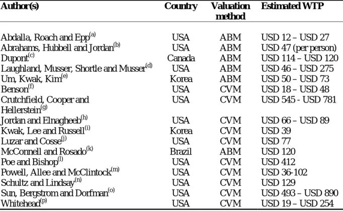
Table 1 presents estimates of WTP (per household, annually) for improvement in water quality from a set of studies.3 This comparison is given for illustrative purposes only because the studies are not directly comparable: the type of contamination and its severity varies across places. For each study, we indicate the authors, the country in which the study took place, the method employed (ABM or Averting Behaviour Method, CVM or Contingent Valuation Method), and the estimated WTP. Estimated WTP varies from USD 12 to USD 890.
Our paper adds to this literature by analyzing WTP for better tap water quality from a household survey made in 10 countries at various stages of development.
3
The list is not exhaustive. For an excellent review and analysis of water quality valuation studies, see Bergstrom, Boyle and Poe (2001).
Table 1. Estimates of WTP for improvement in water safety / quality (per household per year)
Author(s) Country Valuation
method
Estimated WTP
Abdalla, Roach and Epp(a) USA ABM USD 12 – USD 27
Abrahams, Hubbell and Jordan(b) USA ABM USD 47 (per person)
Dupont(c) Canada ABM USD 114 – USD 120
Laughland, Musser, Shortle and Musser(d) USA ABM USD 46 – USD 275
Um, Kwak, Kim(e) Korea ABM USD 50 – USD 73
Benson(f) USA CVM USD 18 – USD 48
Crutchfield, Cooper and Hellerstein(g)
USA CVM USD 545 - USD 781
Jordan and Elnagheeb(h) USA CVM USD 66 – USD 89
Kwak, Lee and Russell(i) Korea CVM USD 39
Luzar and Cosse(j) USA CVM USD 77
McConnell and Rosado(k) Brazil ABM USD 120
Poe and Bishop(l) USA CVM USD 412
Powell, Allee and McClintock(m) USA CVM USD 36-102
Schultz and Lindsay(n) USA CVM USD 129
Sun, Bergstrom and Dorfman(o) USA CVM USD 493 – USD 890
Whitehead(p) USA CVM USD 19 – USD 254
Notes:
(a) Abdalla, Roach and Epp (1992) estimate WTP for reducing the contaminating pollutant (per- and trichloroethylene) to the public drinking water standard levels (in a south-eastern Pennsylvania community, USA).
(b) Abrahams, Hubbell and Jordan (2000) study the effects of risk perceptions, risk information, and perceived water quality on the choice to use water filters or bottled water in Georgia, USA. The survey was conducted in Georgia to study WTP for water quality provisions of the Safe Drinking Water Act.
(c) Dupont (2005) uses surveys on quality perceptions of municipally supplied tap water after the shock following the widespread illnesses caused by the presence of bacteria in drinking water.
(d) Laughland et al. (1996) estimate WTP for reducing the contaminating pollutant (the parasite Giardia lamblia) to the public drinking water standard levels in the USA.
(e) Um, Kwak, and Kim (2002) estimate the WTP of Korean citizens for the change of suspended solid concentration in tap water (to improve the tap water to acceptable levels of pollution), using the conventional and perception ABM.
(f) Benson (2006) uses a CV survey in order to measure the benefits of improved water quality in the Opequon watershed (an area of Virginia, USA). This area is classified as impaired due to violation of bacteria standards. (g) Crutchfield, Cooper and Hellerstein (1997) use CV to value the reduction of nitrate levels in drinking water to safe levels and to completely nitrate-free levels in four regions of the US.
(h) Jordan and Elnagheeb (1993) do CV on a sample of respondents in Georgia, USA, to value the increase above their normal bill that households would pay for a nitrate reduction in groundwater (the main source of drinking water in the region). We report the median WTP for households on public systems and for households using private wells.
(i) Kwak, Lee and Russell (1997) concentrate on drinking water in Korea (municipal and domestic water supply). Respondents are asked if they would need to be compensated for any changes in water quality.
(j) Luzar and Cosse (1998) use data collected from a CV survey of rural residents (USA). The willingness to pay to accept changes in individual and state level water quality is estimated with and without attitudinal explanatory factors.
(k) McConnell and Rosado (2000) estimate the benefits of a discrete improvement in tap water quality in Espírito Santo, Brazil, from households’ use of different types of water filters.
(l) Poe and Bishop (1999) provide information on the actual nitrate levels in the groundwater to respondents in an area in Wisconsin (where groundwater is the sole drinking water source) and use CV to value a 25% decrease in their exposure levels. The table indicates the maximum value of WTP in a cubic function of the incremental benefits.
(m) Powell, Allee and McClintock (1994) investigate the use of CV information as a tool to persuade local government decision makers to implement groundwater protection policies in the USA.
(n)Schultz and Lindsay (1990) elicit household total WTP for a hypothetical groundwater protection plan in the USA. They use a CV survey during the summer of 1988.
(o) Sun, Bergstrom and Dorfman (1992) use CV to estimate the WTP to reduce pesticide and nitrate contamination of groundwater on a sample of households in Georgia, USA. Their estimate, which is very high, is based on an option value model. The mean value on the sample is USD 641 (the confidence interval is given in the Table).
(p) Whitehead (2006) estimates the WTP for improved water quality in North Carolina, USA, using a CV survey.
3. Data and descriptive statistics
3.1. The survey instrument
The data come from the 2008 OECD Survey on Household Environmental Behaviour that aimed at collecting new empirical evidence on attitudes, behaviour and environment in five areas: food, energy, waste, water and personal transport. Respondents were also asked a series of questions regarding characteristics of their household (age, composition, education, income), trustworthiness of information sources, and behavioural attitudes or opinions regarding the environment in general. The purpose of this article is to analyze the respondents’ willingness to pay for water quality. The specific format of the questions on tap water quality is presented in each relevant section below.
The survey was implemented in 10 OECD countries (Australia, Canada, Czech Republic, France, Italy, Korea, Mexico, Netherlands, Norway and Sweden). About 10000 respondents were recruited using a web-based access panel, managed by a private company that specializes in web-based panels. For further details on the survey, we refer the readers to Millock and Nauges (forthcoming).
Web-based surveys are increasingly used as a means to implement targeted surveys at a relatively low cost compared to in-person interviews and are increasingly used in valuation studies (see for example Berrens et al., 2004). Lindhjem and Navrud (2008) recently compared web-based surveys with in-person interviews in a controlled field experiment on the same panel of respondents and found no significant biases in the web-based survey compared to the interview survey. A previous study comparing two different data samples obtained through in-person interviews and through a web survey (invited via email) found that the response rate was lower over the internet, but that the proportion of zero bids was similar in the two samples and that the WTP estimates of the web survey were significantly lower than those obtained through the in-person interview (Marta-Pedroso, Freitas and Domingos, 2007). Olsen (2009) compared two samples obtained through a web-based survey and through mail for a choice experiment, and found similar response rates, but a lower number of protest zero bids in the web survey. The unconditional WTP estimates did not display any statistically significant difference between the samples obtained from the different survey modes. Kiernan et al. (2005) compared a web-based survey with a mail survey and found that the web-based survey had better response rates and the same question completion rate as the mail survey and that there was no evidence of evaluative bias. The same conclusion was reached by Fleming and Bowden (2009) who compared response rates, socio-demographic characteristics, and surplus estimates of respondents obtained from conventional mail and web-based surveys. So far, the results thus seem quite encouraging as to the validity of this type of survey instrument.
3.2 Opinions about tap water quality and WTP measures
In the survey, households were asked whether or not they were satisfied with the quality of their tap water and whether or not they were drinking water from the tap. Households who
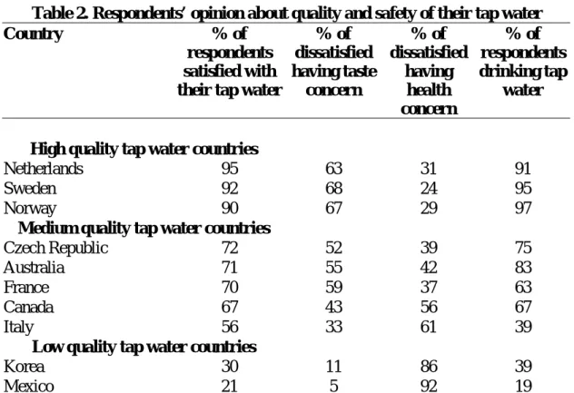
declared being dissatisfied could indicate whether they were more concerned about taste or health impacts (or neither of these), see Table 2.
Table 2. Respondents’ opinion about quality and safety of their tap water
Country % of
respondents satisfied with their tap water
% of dissatisfied having taste concern % of dissatisfied having health concern % of respondents drinking tap water
High quality tap water countries
Netherlands 95 63 31 91
Sweden 92 68 24 95
Norway 90 67 29 97
Medium quality tap water countries
Czech Republic 72 52 39 75
Australia 71 55 42 83
France 70 59 37 63
Canada 67 43 56 67
Italy 56 33 61 39
Low quality tap water countries
Korea 30 11 86 39
Mexico 21 5 92 19
Broadly speaking, we can distinguish three groups of countries. The first group gathers countries where 90% or more of the surveyed respondents declare to be satisfied with the quality of their tap water. The “high quality tap water” group includes the Netherlands (95% of respondents satisfied with their tap water), Sweden (92%) and Norway (90%). In these three countries, more than 90% of the respondents drink tap water. The “medium quality tap water” group gathers countries where the percentage of respondents satisfied with water quality varies between 50 and 75 percent. It includes the Czech Republic (72%), Australia (71%), France (70%), Canada (67%), and Italy (56%). The percentage of respondents drinking tap water varies from a low of 39% in Italy to a high of 83% in Australia. Finally, the “low quality tap water” group gathers Korea and Mexico, where less than 30 percent of
respondents declare to be satisfied with quality of water from the tap. Only 39% [resp. 19%] of the respondents from Korea [resp. Mexico] drink water from the tap. The correlation between the percentage of respondents satisfied with their tap water and the percentage of those drinking tap water is quite high, except for Italy. This finding is not surprising knowing that the annual per capita consumption of bottled water is the highest in this country (see European Federation of Bottled Waters at http://www.efbw.eu/). Drinking bottled water in Italy is a cultural habit that may not be directly linked to the quality of the water provided at the tap. The reasons for being dissatisfied vary from one country to the other. In the “high quality tap water” group, taste is the major concern (for about two-third of the dissatisfied respondents) while health is the primary concern in the “low quality” group gathering Korea and Mexico. In the “medium quality” group, the concerns are slightly more balanced, except in Italy where the health concern dominates. These simple statistics indicate that we should expect significantly different WTP for better tap water quality from one country to another.
Only those respondents who declared NOT being satisfied with their tap water were asked how much they would be willing to pay for improvement. More precisely, the analysis of respondents’ WTP for better tap water quality is based on the answer to the following question: “What is the maximum percentage increase that you would be willing to pay above
your actual water bill to improve the quality of your tap water, holding water consumption constant?”. The six possible answers were: (1) nothing, (2) less than 5%, (3) between 5% and
15%, (4) between 16% and 30%, (5) more than 30%, and (97) don’t know. On the pooled sample, 34% of the respondents were not willing to pay anything above their actual bill to get improved water quality, 29% were willing to pay less than 5%, 22% were willing to pay between 5 and 15%, 5% of the respondents were willing to pay between 16% and 30%, and
less than 2% of the respondents were willing to pay more than 30% above their actual bill. 9% of the respondents declared that they “do not know”.
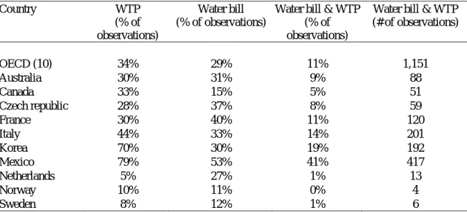
Due to the survey design which implies that respondents stated their WTP for an improved water quality only if they declared not being satisfied with the quality of their tap water for drinking, we miss data on WTP for a large number of respondents. About 66% of households in the original sample declared being satisfied with water at the tap and hence did not answer the subsequent WTP question. For those households who answered the WTP question, we need reliable information on the amount paid for water each year in order to monetize WTP (which was stated as a percentage of the annual water bill). In the questionnaire, households were asked to take out their water bills and state their total annual cost of water consumption and the corresponding annual consumption. The latter, unfortunately, was not provided by all respondents. Table A1 in Appendix indicates the percentage of non-missing data for the annual water bill and WTP, for the pooled data, and country by country. Only about 11% of the original sample answered both the WTP question and the question on the annual water bill, which drastically reduces the data to analyse WTP (from 10251 to 1151 observations). In order to lessen the problem of missing values and of limited respondent awareness of the water bill, we decided to build “representative water bills” by country and by household type, where household type is defined by its size and localization. We consider two categories for household size: two members or less, and at least three members; and three categories for household habitat (rural, suburban, urban). For each of the six household types, and each country, we compute the median annual water bill.4 The monetary bound values (EUR) of the
4
For respondents who stated their water consumption but not their water bill, we calculate their water bill by multiplying the stated consumption by the median water price in their country. Water price is computed as the ratio of the annual water bill over the annual water consumption. We considered as out of range any stated annual water use below 50 m3 or above 4000 m3 (any observation falling outside these bounds was removed from the sample). Once the data have been cleaned, we computed the median water price and the median water
WTP are then derived by multiplying the percentage bounds by the median bill, for each household type and each country. Data availability is roughly doubled since WTP can now be computed for 3329 respondents. WTP is interpolated as the mid-point in the interval, producing a single monetary WTP value. As for the upper interval (more than 30%), we impute the conservative, but realistic, value of 30% for these respondents (lower bound).5
3.3. Descriptive statistics
In addition to health/taste concern, the survey contains information on the respondent’s socio-economic, behavioral and attitudinal characteristics. The following variables are expected to influence WTP for better tap water quality:
i) socioeconomic characteristics including household income, age, gender, and education level of the respondent. Income falls into four classes, class 1 [resp. class 4] gathering households with the lowest [resp. highest] income. We also control for households who did not answer the question on income (class 5).
ii) two indicator variables describing whether the respondent devotes time to an environmental organization (variable i_time_orga) and whether the respondent is a member of or has donated money to such organizations (variable i_member_orga).
iii) an index measuring environmental concern in general (not just concerning water quality), that could be interpreted as a proxy for the perception of a general environmental threat. For each of the following environmental issues (waste generation, air pollution, climate change, water pollution, natural resource depletion, genetically modified organisms, endangered
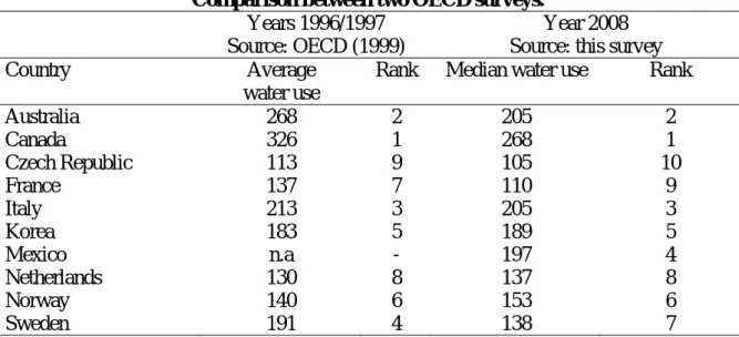
use, for each country in our sample. These figures are found to be close enough to country statistics provided by the OECD in 1999 and 2003 to provide good confidence in our data (Tables A4 and A5 in Appendix).
5
For example, consider that a respondent living alone in a suburban habitat in Mexico has stated that he would be willing to pay as a maximum between 5% and 15% of his water bill to get a better tap water quality. In Mexico, the median annual water bill for a household with two members or less and living in a suburban area is 82 EUR. We thus consider that this respondent is willing to pay 10% x 82 = 8.2 EUR for better tap water quality.
species and biodiversity, noise), respondents had to state whether they were not concerned (1), fairly concerned (2), concerned (3), very concerned (4), or had no opinion (5). We calculate the mean score for each respondent on the answers coded from 1 to 4 (we do not consider in the computation the case of answers equal to 5).6 A higher value of the index indicates a higher degree of environmental consciousness or commitment.7
iv) trust in government regarding information on environmental issues. Respondents had to rank the following sources of information in terms of their trustworthiness: independent researchers and experts, national/local governments, environmental non-governmental organisations (NGOs), consumers’ organisations, and producers’ and retailers’ associations. We build a variable (notrust_gov) which corresponds to the rank attributed to national/local governments such that a higher value of the index indicates less confidence.
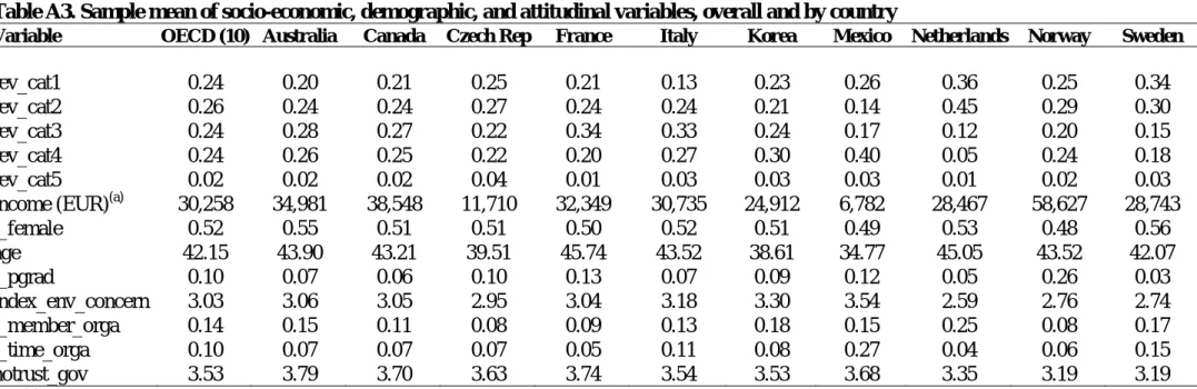
The list of explanatory factors that are used in the econometric analyses and the sample mean of each variable (for the entire sample and for each country separately) are given in Appendix (Table A2 and Table A3 respectively).
6
See Lam (2006) for a similar approach. We also tried to build an index using Principal Component Analysis (PCA) but the index built following the sample mean approach was found to be more significant in general. Factor analysis would be another possible technique for aggregating answers measured on a Likert scale (Gilg and Barr, 2006).
7
This index will be treated as a continuous variable, which relies on the underlying assumption that the ordering is linear. In other words, we assume that moving from “not concerned” to “fairly concerned” is equivalent to a move from “fairly concerned” to “concerned”. Instead, one could have considered separately the answer to each separate item and build dummy variables corresponding to each answer and each item. This procedure would, however, increase significantly the number of parameters to be estimated in the model.
4. Empirical analysis
4.1. Estimation procedure and results
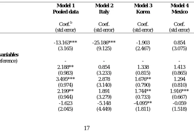
For now, we consider that respondents who are dissatisfied with water quality but “do not know” how much they would be willing to pay for improved water quality, are indeed willing to pay nothing (see Haab and McConnell, 2002). The sensitivity of our estimates to this assumption will be discussed in the following section. To control for biases induced by the censored nature of the WTP variable, the model is estimated using a Tobit approach. The Tobit model was first estimated on the pooled data and then separately for each of the three countries with the highest percentage of respondents dissatisfied with their tap water, namely Italy, Korea and Mexico. The number of observations for the other countries was too small to allow for a country-by-country analysis. Multicollinearity was tested by checking the condition number of the matrix of independent variables (see Belsley, Kuh and Welsch, 1980). The results are given in Table 3.
Table 3. Estimation results from the Tobit models –
Model on the pooled data and separate models for Italy, Korea and Mexico. Model 1 Model 2 Model 3 Model 4 Pooled data Italy Korea Mexico
Variablesa Coef.b (std error) Coef. (std error) Coef. (std error) Coef. (std error) Constant -13.163*** (3.165) -25.186*** (9.125) -1.903 (2.467) 0.854 (3.075) Economic variables rev_cat1 (reference) - - - - rev_cat2 2.188** (0.983) 0.854 (3.233) 1.338 (0.815) 1.413 (0.865) rev_cat3 3.495*** (0.974) 2.878 (3.140) 1.676** (0.790) 1.294 (0.810) rev_cat4 2.199** (0.944) 1.891 (3.279) 1.744** (0.733) 1.916*** (0.667) rev_cat5 -1.623 (2.045) -5.148 (4.449) -4.095** (1.811) -0.059 (1.518)
Demographic variables i_female -2.590*** (0.661) -5.912*** (1.923) -0.558 (0.533) -0.388 (0.538) age -0.148*** (0.024) -0.137** (0.065) 0.016 (0.197) -0.012 (0.024) i_pgrad 3.165*** (1.120) 4.234 (3.355) 0.769 (0.925) 0.498 (0.805) Attitudinal characteristics index_env_concern 1.984*** (0.621) 2.020 (1.905) -0.016 (0.512) -0.341 (0.761) i_member_orga 4.076*** (0.998) 7.620** (3.034) 1.584** (0.743) 0.641 (0.842) i_time_orga 2.094* (1.082) 5.295* (2.132) 0.939 (1.154) 1.464** (0.663) notrust_gov -0.429* (0.251) -0.770 (0.731) 0.020 (0.187) -0.011 (0.206) Household’s opinion i_taste_concern 10.013*** (2.034) 29.842*** (7.368) 1.974 (1.819) 2.752 (2.008) i_health_concern 11.258*** (1.989) 32.884*** (7.316) 1.749 (1.647) 4.282** (1.669) Country dummies i_Australia (reference) - - - - i_Canada 4.780** (1.628) - - - i_Czech 7.318*** (1.850) - - - i_France 1.120 (1.678) - - - i_Italy 7.279*** (1.458) - - - i_Korea -0.576 (1.490) - - - i_Mexico 3.124** (1.517) - - - i_Netherlands -6.006* (3.366) - - - i_Norway 3.543 (2.326) - - - i_Sweden 14.901*** (2.431) - - -
Test of global significance
LR Chi2(22) = 260.06 p-value = 0.0000 LR Chi2(13) = 61.60 p-value = 0.0000 LR Chi2(13) = 33.91 p-value = 0.0010 LR Chi2(13) = 27.38 p-value = 0.0067 Number of observations 3158 577 626 720
Number of censored observations 1316 244 225 151
a) The prefix i_ indicates a 0/1 variable.
First, in Model 1 on pooled data, the revenue coefficients are positive and statistically significant at a 1% or 5% level, except for category 5 which represents respondents who did not answer the question on income. Category 1, which gathers the lowest incomes, is the reference category. Compared to revenue category 1, respondents who are members of households who earn higher revenues have a higher WTP for improvement in the drinking water quality. Second, the attitudinal characteristics are found to be significant, with the expected positive signs: respondents with a greater environmental concern as well as respondents who devote time to environmental organization and donate money to such organizations have on average a higher WTP for drinking water quality.8 Interestingly, trust in information from national or local governments is found to be positively related to the WTP. Third, the willingness to pay is decreasing with age. This result has been found by several other authors (see for example Abrahams, Hubbell and Jordan, 2000; Um, Kwak and Kim, 2002), although Luzar and Cosse (1998) suggest the relationship may be nonlinear (they obtain a negative sign on age and a positive sign on age-squared). We tested a nonlinear effect of age but it was not significant, neither in the pooled sample, nor in the country estimations. Women are found to have a lower willingness to pay for a better drinking water quality, and respondents with a high education level (about 9% of the whole sample) seem to be willing to pay more for water quality. Higher education is normally expected to be positively related to willingness to pay, but previous research does not always find it significant. The results on gender are also mixed in the literature. On the other hand, the presence of young children in the household has been shown to increase the willingness to pay for water quality (Abdalla, Roach and Epp, 1992; Luzar and Cosse, 1998). In our analysis, though, the presence of young
8
We also estimated the WTP model by replacing the index of environmental concern (index_env_concern) with indicator variables describing the respondent’s concern about water pollution, the item which was directly related to the question studied. We considered one indicator variable for each possible answer: not concerned (1), fairly concerned (2), concerned (3), very concerned (4), or had no opinion (5). None of these indicators were found significant.
children - or other variables related to the composition of the household - was never significant in the estimations.
The country coefficients are significant (at a level of 1%, 5% or 10%) except for France, Korea and Norway (the reference country is Australia). The country effects should capture differences in the water provision infrastructure, regulatory standards for water quality, and cultural differences or habit in drinking water from the tap. The positive sign and the magnitude of the coefficient for Sweden is surprising. Knowing that WTP in our model is measured in absolute value, the large coefficient for Sweden may be explained by the high drinking water price in this country (a high water price implies a high water bill and hence a high WTP since the latter is stated as a percentage of the water bill) compared to other OECD countries (see Table A5 in Appendix). A recent survey conducted by Istat (2006) indicated that more than a third of Italians do not trust the water supplied by operators and about a sixth complains of irregular water supply (disruptions, shifts in supply, rationing), which may explain the positive sign and the magnitude of the country-specific coefficient for Italy. In Canada, the high country-specific effect may be the consequence of several water contamination incidents in the past that have caused severe casualties. In Mexico, a history of federally subsidized water service and poor financing, while encouraging economic development, has limited the capacity of the government to expand the network, treat water and wastewater, and fund repairs (Tortajada, 2006). A relatively low quality of the service combined with a currently low price of water may explain customers’ WTP for a better tap water quality. The only slightly surprising result is the negative but non-significant effect for a location in Korea. We expected a positive and significant effect for this country: the National Survey on Public Awareness for Environmental Conservation (Korean Ministry of the Environment, 2008) indicated that 37% of the respondents were satisfied with quality of the
water at the tap but only 1.4% were drinking tap water directly. The rest either boiled water (44%), filtered water (42%), bought bottled water (8%), or used water from wells or other sources (5%). Korean households are not satisfied with tap water but are used to incur expenditures to cope with the bad quality of the water (see also Um, Kwak and Kim, 2002), which may explain their reluctance to pay a higher price for water provided at the tap.
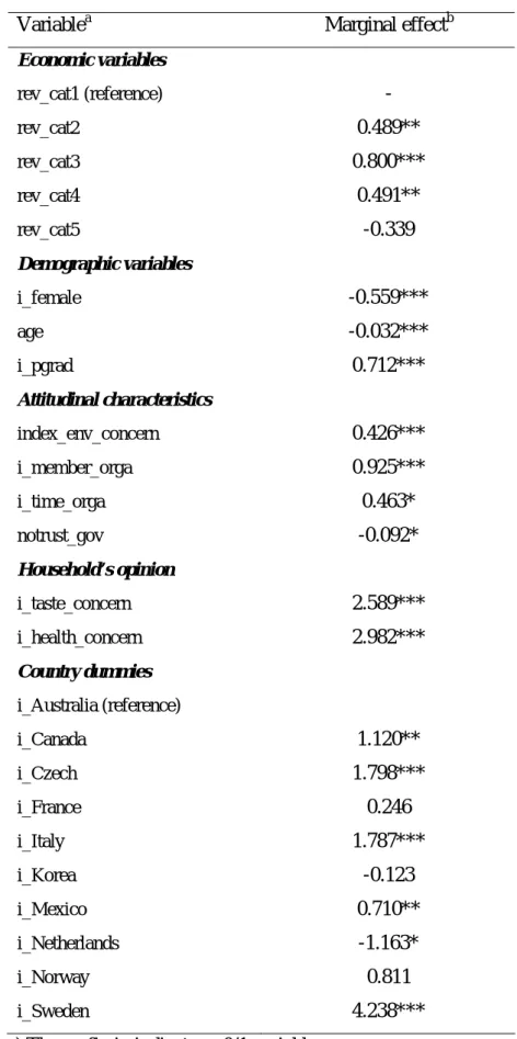
The impact of these variables is better illustrated by marginal effects (see Table 4): our results indicate that moving from the lowest income category to the category just above yields an increase in WTP of 50 euro-cents. Education has at least as important an impact on WTP as revenue. The effect of the attitudinal variables are at least equal to moving from one revenue category to another, and in some cases, even larger. More precisely, and not surprisingly, the computation of marginal effects shows that respondents who are contributors/donors to an environmental organization exhibit a greater WTP (about EUR 1) than the others. Amongst respondents concerned with water quality, those with taste or health concerns are willing to pay about EUR 2.6 more than those with other concerns.9 This is as expected and in line with previous results on concern with health effects (for example Sun, Bergstrom and Dorfman, 1992).
9
Computed test statistics indicate no significant difference in the marginal effect on WTP of health concerns compared to taste concerns.
Table 4. Estimated marginal effects (pooled sample)
Variablea Marginal effectb
Economic variables rev_cat1 (reference) - rev_cat2 0.489** rev_cat3 0.800*** rev_cat4 0.491** rev_cat5 -0.339 Demographic variables i_female -0.559*** age -0.032*** i_pgrad 0.712*** Attitudinal characteristics index_env_concern 0.426*** i_member_orga 0.925*** i_time_orga 0.463* notrust_gov -0.092* Household’s opinion i_taste_concern 2.589*** i_health_concern 2.982*** Country dummies i_Australia (reference) i_Canada 1.120** i_Czech 1.798*** i_France 0.246 i_Italy 1.787*** i_Korea -0.123 i_Mexico 0.710** i_Netherlands -1.163* i_Norway 0.811 i_Sweden 4.238***
a) The prefix i_ indicates a 0/1 variable.
The country specific estimation results exhibit similarities with the pooled data results. However, the coefficients are less significant in general. Furthermore, the revenue categories appear to be significant for the low income countries (Korea, Mexico), whereas they are not for the high income country (Italy). The opposite seems to be true for the attitudinal characteristics, suggesting that these characteristics mainly play a role in rich countries.
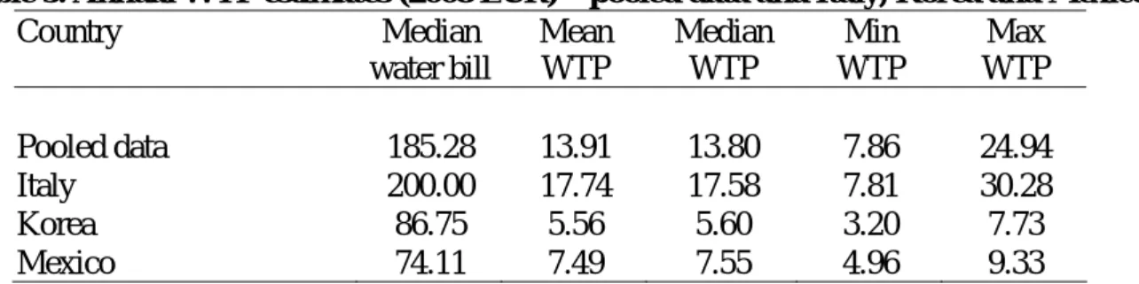
The estimated parameters of the four models were used to assess the willingness to pay for an improved drinking water quality (see Table 5).10 The mean and median values for the pooled data (EUR 14 or USD 21 per household) represent about 7.5% of the median annual water bill. At the country level, the median WTP in Italy, Korea and Mexico represents respectively 8.8%, 6.4% and 10.1% of the median water bill. The highest relative WTP is, without any surprise, observed in the country with the highest number of dissatisfied respondents (Mexico).11 However, cross-country comparisons have to be made with caution. Indeed, the main question used to measure WTP for improved tap water quality is very general and may have different interpretations from one country to another according to the specific water quality problems and quality benchmarks of each country.
The average estimated WTP is lower than the WTP obtained by Abrahams, Hubbell, and Jordan (2000): USD 47 per person and per year. It may also seem low in comparison with households’ expenditures on bottled water. A recent study made in France indicated that an
10
We provide non-conservative WTP estimates, i. e., estimates based on the truncated data, rather than based on the censored data.
11
We performed a conditional moments test, using the user-written tobcm command (Drukker, 2002), to test for the null hypothesis that the error terms in our model are normally distributed. The normality assumption was rejected, which could cast doubt on the robustness of our Tobit estimates. Following Cameron and Trivedi (2005), we estimated the WTP model using competing approaches including the estimation of a selection model (two-step version of the Heckman estimator) and a two-part model (Probit model to explain the zeroes, Ordinary Least Squares applied on the positive values) which is less sensitive to the normality assumption. The WTP estimates are found to be robust to the chosen econometric methodology and we are thus confident about the WTP estimates obtained from the Tobit. The full set of estimation results is not shown here but is available from the authors upon request.
individual drinks about 0.5 litre per day and that the price of bottled water is approximately EUR 0.28 per litre (Bontemps and Nauges, 2009). A rough calculation shows that the annual consumption of bottled water would be 475 litres per year and would cost around EUR 133 for a household not drinking tap water (or equivalently USD 75 per person per year), which is far higher than the estimates presented here.
Table 5. Annual WTP estimates (2008 EUR) – pooled data and Italy, Korea and Mexico Country Median water bill Mean WTP Median WTP Min WTP Max WTP Pooled data 185.28 13.91 13.80 7.86 24.94 Italy 200.00 17.74 17.58 7.81 30.28 Korea 86.75 5.56 5.60 3.20 7.73 Mexico 74.11 7.49 7.55 4.96 9.33 4.2. Robustness checks
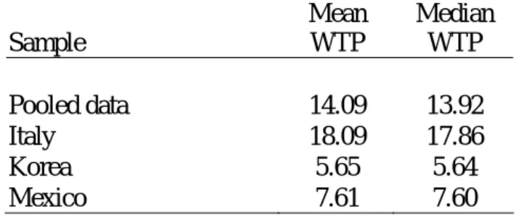
As discussed earlier, these estimates have been obtained under the assumption that respondents who “do not know” are willing to pay nothing for improved tap water quality (on a sample of 3158 observations). This assumption implies a conservative estimate of WTP. We test the robustness of the WTP estimates relative to this assumption by re-computing WTP on the sample for which respondents who do not know have been withdrawn. The restricted sample has 2893 observations. Mean and median estimated WTP are found to be quite robust to the specification (see Table 6).
Table 6. Annual WTP estimates (2008 EUR) – Restricted sample Sample Mean WTP Median WTP Pooled data 14.09 13.92 Italy 18.09 17.86 Korea 5.65 5.64 Mexico 7.61 7.60
Up to now, WTP has been computed based on the sub-sample of respondents who declared not being satisfied with water quality at the tap. One could consider that respondents who expressed satisfaction with water quality are willing to pay zero for quality improvement. We re-estimated the WTP model on the entire sample of respondents (9285 observations overall). The estimates are not directly comparable since the latter model does not include the indicator variables describing households’ concern about health and taste (variables called
i_taste_concern and i_health_concern). This is because the question about health and taste
was not asked to the respondents who declared being satisfied with the water quality. The mean WTP is estimated at EUR 11.90, which is not that far from the WTP that was estimated on the sub-sample of respondents who declared not being satisfied with water quality at the tap (see Table 7).
Table 7. Summary: Annual WTP estimates (2008 EUR) on the three samples
Sample used to estimate WTP Number of
observations
Mean WTP, 2008 EUR Subsample of non-satisfied respondents;
“Do not know” implies WTP=0 3158 13.91
Sub-sample of non-satisfied respondents:
“Do not know” excluded 2893 14.09
5. Conclusions
The analysis of households’ willingness to pay for improved water quality indicates that households are on average willing to pay rather small amounts for better tap water quality: for the pooled data the WTP represents 7.5% of the median annual water bill. On the pooled sample, this represents a range of WTP from EUR 7 to 24 (or equivalently from USD 10 to 35) annually per household. The cross-country comparison has to be made with caution, though, because of the specific water quality benchmarks of each country.
These estimates are lower than the ones obtained by Abrahams, Hubbell, and Jordan (2000) on the US and McConnell and Rosado (2000) on Brazil: USD 47 per person per year and USD 120 per household per year, respectively. The discrepancy in the WTP estimates is probably explained by the specificity of each region and the method employed (Averting Behaviour Model for the studies in the US and Brazil, and Contingent Valuation for the 10 OECD countries). Further research is needed to get greater confidence in the WTP for improved tap water quality.
Finally, our results indicate the need for further analysis of the set-up of the water provision infrastructure. In particular, it would be useful to include measures not only of the respondents’ general perception of the quality of their tap water, but rather the level of and the exceedance of the regulatory standards and type of water provision and organization. More elaborate measures of trust in the supplier could usefully be included in future surveys.
Acknowledgements
The data upon which this study is based were collected as part of the OECD’s project ‘‘Household Behaviour and Environmental Policy’’ (www.oecd.org/env/cpe/consumption). This work is published on the responsibility of the authors. The opinions expressed and arguments employed herein do not necessarily reflect the official views of the OECD and/or of the governments of its member countries. The authors are grateful to the OECD for providing the data.
References
Abdalla, C.W., B.A. Roach and D.J. Epp, 1992. Valuing Environmental Quality Changes Using Averting Expenditures: An Application to Groundwater Contamination. Land
Economics 68(2), 163-169.
Abrahams, N.A, B.J. Hubbell and J.L. Jordan, 2000. Joint Production and Averting Expenditure Measures of Willingness to Pay: Do Water Expenditures Really Measure Avoidance Costs? American Journal of Agricultural Economics 82(2), 427-437.
Belsley D.A., E. Kuh, and R.E. Welsch, 1980. Regression Diagnostics, Wiley, New-York.
Benson, M.C., 2006. An Economic Valuation of Improved Water Quality in Opequon Watershed. Thesis submitted to the Davis College of Agriculture, Forestry, and Consumer Sciences at West Virginia University, Master of Science in Agricultural and Resource Economics, Division of Resource Management, Morgantown, West Virginia.
Bergstrom, J.C., K.J. Boyle and G.L. Poe, 2001. The Economic Value of Water Quality, Cheltenham: Edward Elgar Publishing.
Berrens, R.P., A.K. Bohara, H.C. Jenkins-Smith, C.L. Silva and D.L. Weimer, 2004. Information and Effort in Contingent Valuation Surveys: Application to Global Climate Change Using National Internet Samples. Journal of Environmental Economics and
Management 47, 331-363.
Birol, E., P. Koundouri and Y. Kountouris, 2008. Using Economic Valuation Techniques to Inform Water Resource Management in the Southern European Mediterranean, and Developing Countries: A Survey and Critical Appraisal of Available Techniques, In P. Koundouri (Ed.), Coping with Water Deficiency, Springer, pp. 135-155.
Bontemps, C. and C. Nauges, 2009. Carafe ou bouteille? Le role de l’environnement dans la décision du consommateur (Tap or Bottled Water ? The Role of Environmental Quality in the Consumer’s Decision). Economie et Prévision 188, 61-79.
Camerer, C., 1995. Individual Decision Making. In J. Kagel and A. Roth (Eds.),
Handbook of Experimental Economics, Princeton, NJ: Princeton University Press, 1995,
587-703.
Cameron A. C. and P. K. Trivedi, 2005. Microeconometrics: Methods and Applications. Cambridge: Cambridge University Press.
Courant, P.N., and R.C. Porter, 1981. Averting Expenditure and the Cost of Pollution.
Journal of Environmental Economics and Management 8(4), 321-329.
Crutchfield, S.R., J.C. Cooper and D. Hellerstein, 1997. Benefits of Safer Drinking Water: The Value of Nitrate Reduction. Agricultural Economic Report No. 752, US Department of Agriculture, Economic Research Service, Food and Consumer Economics Division, Washington, D.C.
Danielson, L., T.J. Hoban, G. van Houtven, and J.C. Whitehead, 1995. Measuring the benefits of local public goods: Environmental quality in Gaston County, North Carolina.
Drukker, D.M., 2002. Bootstrapping a Conditional Moments Test for Normality after Tobit Estimation. The Stata Journal 2: 125-139.
Dupont, D.P., 2005. Tapping into Consumers’ Perceptions of Drinking Water Quality in Canada: Capturing Customer Demand to Assist in Better Management of Water Resources.
Canadian Water Resources Journal 30(1), 11-20.
Fleming, C.M. and M. Bowden, 2009. Web-Based Surveys as an Alternative to Traditional Mail Methods. Journal of Environmental Management 90(1), 284-292.
Gilg, A., and S. Barr, 2006. Behavioural Attitudes towards Water Saving? Evidence from a Study of Environmental Actions. Ecological Economics 57(3), 400-414.
Haab, T.C., and K.E. McConnell, 2002. Valuing Environmental and Natural Resources,
The Econometrics of Non-Market Valuation. Edward Elgar, New Horizons in Environmental
Economics Series.
Harrington, W., A.J. Krupnick and W.O. Spofford, 1989. The Economic Losses of a Waterborne Disease Outbreak. Journal of Urban Economics 25(1), 116-137.
ISTAT, 2006. Indagine multiscopo sulle famiglie “Aspetti della vita quotidiana”, 2005, Roma.
Jardine, C.G., N. Gibson, and S. Hrudey, 1999. Detection of Odour and Health Risk Perception of Drinking Water. Water Science and Technology 40(6), 91-98.
Jordan, J.L. and A.H. Elnagheeb, 1993. Willingness to Pay for Improvements in Drinking Water Quality. Water Resources Research 29(2), 237–245.
Kiernan, N.E., M. Kiernan, M.A. Oyler and C. Gilles, 2005. Is a Web Survey as Effective as a Mail Survey? A Field Experiment among Computer Users. American Journal of
Kwak, S.J, J. Lee, and C.S. Russell, 1997. Dealing with Censored Data from Contingent Valuation Surveys: Symmetrically-Trimmed Least Squares Estimation. Southern Economics
Journal 63(3): 743-750.
Lam, S.P., 2006. Predicting Intention to Save Water: Theory of Planned Behavior, Response Efficacy, Vulnerability, and Perceived Efficiency of Alternative Solutions. Journal
of Applied Social Psychology 36(11), 2803-2824.
Laughland, A.S, W.N. Musser, J.S. Shortle and L.M. Musser, 1996. Construct Validity of Averting Cost Measures of Environmental Benefits. Land Economics 72(1), 100-112.
Levallois, P., J. Grondin, and S. Gingras, 1999. Evaluation of Consumer Attitudes on Taste and Tap Water Alternatives in Québec. Water Science and Technology 40(6), 135-39.
Lindhjem, H. and S. Navrud, 2008. Internet CV surveys – A Cheap Fast Way to Get Large Samples of Biased Values? MPRA Paper No. 11471. Online at http://mpra.ub.uni-muenchen.de/11471/
Luzar, E.J, and K.J. Cosse, 1998. Willingness to Pay or Intention to Pay: The Attitude-Behavior Relationship in Contingent Valuation. Journal of Socioeconomics 27(3), 427-444.
Marta-Pedrosa, C., H. Freitas and T. Domingos, 2007. Testing for the Survey Mode Effect on Valuation Data Quality: A Case Study of Web Based versus In-Person Interviews.
Ecological Economics 62, 388-398.
McConnell, K.E., and M.A. Rosado, 2000. Valuing Discrete Improvements in Drinking Water Quality through Revealed Preferences. Water Resources Research 36(6), 1575-1582.
Millock, K., and C. Nauges, forthcoming. Household Adoption of Water-Efficient Equipment: The Role of Socio-economic Factors, Environmental Attitudes and Policy.
Olsen, S.B., 2009. Choosing Between Internet and Mail Survey Modes for Choice Experiment Surveys Considering Non-Market Goods. Environmental and Resource
Economics 44, 591-610.
OECD, 1999. The Price of Water: Trends in OECD Countries. Organisation for Economic Co-Operation and Development, Paris.
OECD, 2003. Social Issues in the Provision and Pricing of Water Services. Organisation for Economic Co-Operation and Development, Paris.
Poe, G.L., and R. C. Bishop, 1999. Valuing the Incremental Benefits of Groundwater Protection when Exposure Levels are Known. Environmental and Resource Economics 13, 341-367.
Powell, J.R., D.J. Allee, and C. McClintock, 1994. Groundwater Protection Benefits and Local Community Planning: Impact of Contingent Valuation Information. American Journal
of Agricultural Economics 76(5), 1068-1075.
Schultz, S.D. and B.E. Lindsay, 1990. The Willingness to Pay for Groundwater Protection. Water Resources Research 26(9), 1869-1875.
Slovic, P., 2000. The Perception of Risk. London: Earthscan.
Sun, H., J.C. Bergstrom and J.H. Dorfman, 1992. Estimating the Benefits of Groundwater Pollution Control. Southern Journal of Agricultural Economics 24(2), 63-71.
Tortajada, C., 2006. Water Management in Mexico City Metropolitan Area. Water
Resources Development 22(2), 353-376.
Turgeon, S., M.J. Rodriguez, M. Thériault, and P. Levallois, 2004. Perception of Drinking Water in the Quebec City Region (Canada): the Influence of Water Quality and Consumer Location in the Distribution System. Journal of Environmental Management 70, 363-73.
Um, M.J., S.J. Kwak, and T.Y. Kim, 2002. Estimating Willingness to Pay for Improved Drinking Water Quality Using Averting Behavior Method with Perception Measure.
Environmental and Resource Economics 21(3), 287-302.
Whitehead J.C., 2006. Improving Willingness to Pay Estimates for Quality Improvements through Joint Estimation with Quality Perceptions. Southern Economic Journal 73(1), 100-111.
Worthington, A.C., and M. Hoffman, 2008. An Empirical Survey of Residential Water Demand Modelling. Journal of Economic Surveys 22(5), 842-871.
Appendices
Appendix A
Table A1. Available information for WTP, water bill, and both questions combined
Country WTP (% of
observations)
Water bill (% of observations)
Water bill & WTP (% of observations)
Water bill & WTP (# of observations) OECD (10) 34% 29% 11% 1,151 Australia 30% 31% 9% 88 Canada 33% 15% 5% 51 Czech republic 28% 37% 8% 59 France 30% 40% 11% 120 Italy 44% 33% 14% 201 Korea 70% 30% 19% 192 Mexico 79% 53% 41% 417 Netherlands 5% 27% 1% 13 Norway 10% 11% 0% 4 Sweden 8% 12% 1% 6
Table A2. List of explanatory factors
Variable names Variable definitions
Economic variables
rev_cat1 Household revenue category 1 (lowest income group) rev_cat2 Household revenue category 2
rev_cat3 Household revenue category 3
rev_cat4 Household revenue category 4 (highest income group)
rev_cat5 Equal to 1 if the respondent does not want to answer on income
Demographic variables
i_female Equal to 1 if the respondent is female
age Age of the respondent
i_pgrad Equal to 1 if the respondent holds a post graduate degree
Household’s opinion about water at the tap
i_taste_concern Equal to 1 if the respondent is most concerned about the taste of the tap water
i_health_concern Equal to 1 if the respondent is most concerned about the safety of the tap water
Attitudinal characteristics
index_env_concern Index of concern about environmental issues
i_time_orga Equal to 1 if the respondent has invested some personal time to support or participate in an environmental organization
i_member_orga Equal to 1 if the respondent is currently a member of, or contributor/donator to, any environmental organisations notrust_gov
Categorical variable: ranks the local/national government sources of information on environmental issues 1 stands for the most trustworthy and 5 for the least trustworthy
Table A3. Sample mean of socio-economic, demographic, and attitudinal variables, overall and by country
Variable OECD (10) Australia Canada Czech Rep France Italy Korea Mexico Netherlands Norway Sweden
rev_cat1 0.24 0.20 0.21 0.25 0.21 0.13 0.23 0.26 0.36 0.25 0.34
rev_cat2 0.26 0.24 0.24 0.27 0.24 0.24 0.21 0.14 0.45 0.29 0.30
rev_cat3 0.24 0.28 0.27 0.22 0.34 0.33 0.24 0.17 0.12 0.20 0.15
rev_cat4 0.24 0.26 0.25 0.22 0.20 0.27 0.30 0.40 0.05 0.24 0.18
rev_cat5 0.02 0.02 0.02 0.04 0.01 0.03 0.03 0.03 0.01 0.02 0.03
income (EUR)(a) 30,258 34,981 38,548 11,710 32,349 30,735 24,912 6,782 28,467 58,627 28,743
i_female 0.52 0.55 0.51 0.51 0.50 0.52 0.51 0.49 0.53 0.48 0.56 age 42.15 43.90 43.21 39.51 45.74 43.52 38.61 34.77 45.05 43.52 42.07 i_pgrad 0.10 0.07 0.06 0.10 0.13 0.07 0.09 0.12 0.05 0.26 0.03 index_env_concern 3.03 3.06 3.05 2.95 3.04 3.18 3.30 3.54 2.59 2.76 2.74 i_member_orga 0.14 0.15 0.11 0.08 0.09 0.13 0.18 0.15 0.25 0.08 0.17 i_time_orga 0.10 0.07 0.07 0.07 0.05 0.11 0.08 0.27 0.04 0.06 0.15 notrust_gov 3.53 3.79 3.70 3.63 3.74 3.54 3.53 3.68 3.35 3.19 3.19
Table A4. Water consumption (litre per day per capita). Comparison between two OECD surveys.
Years 1996/1997
Source: OECD (1999)
Year 2008 Source: this survey Country Average
water use
Rank Median water use Rank
Australia 268 2 205 2 Canada 326 1 268 1 Czech Republic 113 9 105 10 France 137 7 110 9 Italy 213 3 205 3 Korea 183 5 189 5 Mexico n.a - 197 4 Netherlands 130 8 137 8 Norway 140 6 153 6 Sweden 191 4 138 7
Table A5. Water price per m3 (EUR). Comparison between two OECD surveys.
Years 1999-2001
Source: OECD (2003)
Year 2008 Source: this survey Country Average price Rank Median price Rank Australia 1.62 5 0.65 8 Canada 0.72 7 1.06 6 Czech Rep. 1.07 6 1.44 5 France 2.65 4 2.80 1 Italy 0.67 8 0.94 7 Korea n.a. - 0.42 9 Mexico 0.28 9 0.30 10 Netherlands 3.39 2 1.76 3 Norway 5.41 1 1.52 4 Sweden 2.68 3 2.36 2
Appendix B. Selected questions from the OECD Household Survey
Part G - WATER
The following section will cover water consumption and use.
87. Is your household charged for water consumption in your primary residence?
1. Yes 2. No 3. Not sure
88. What would best describe your situation in your primary residence?
1. Not connected to the mains water (using a well/bore, a rainwater tank) 2. Connected to the mains water but not charged for water consumption 3. Don’t know
89. How is your household charged for water consumption?
1. Charged according to how much water is used (e.g. via a water meter) 2. Flat fee (e.g. lump sum included in charges or rent)
3. Don’t know
90. Approximately how much was the total annual cost for water consumption for your primary residence?
Please indicate if possible amount in $ and corresponding annual consumption in m³
Amount in $ per year
Please provide answer to the nearest dollar Volume of water consumed in m³ Don’t know
…
95a. Do you drink tap water for your normal household consumption?
1. Yes 2. No
95. Are you satisfied with the quality of your tap water for drinking?
1. Yes 2. No
96. In your tap water, what is of most concern to you?
1. Taste
2. Concern about health impacts 3. Neither of these
97. What is the maximum percentage increase you would be willing to pay above your actual water bill to improve the quality of your tap water, holding water consumption constant? 1. Nothing 2. Less than 5% 3. Between 5% and 15% 4. Between 16% and 30% 5. More than 30% 6. Don’t know