Tight-binding modelling of ferromagnetic metals and alloys

HAL Id: hal-01720305

https://hal-amu.archives-ouvertes.fr/hal-01720305

HAL is a multi-disciplinary open access archive for the deposit and dissemination of sci-entific research documents, whether they are pub-lished or not. The documents may come from teaching and research institutions in France or abroad, or from public or private research centers.

L’archive ouverte pluridisciplinaire HAL, est destinée au dépôt et à la diffusion de documents scientifiques de niveau recherche, publiés ou non, émanant des établissements d’enseignement et de recherche français ou étrangers, des laboratoires publics ou privés.

Distributed under a Creative Commons Attribution - NonCommercial - NoDerivatives| 4.0

Tight-binding modelling of ferromagnetic metals and

alloys

M Sansa, A Dhouib, F. Ribeiro, B. Legrand, G. Tréglia, C. Goyhenex

To cite this version:

M Sansa, A Dhouib, F. Ribeiro, B. Legrand, G. Tréglia, et al.. Tight-binding modelling of ferro-magnetic metals and alloys. Modelling and Simulation in Materials Science and Engineering, IOP Publishing, 2017, 25 (8), �10.1088/1361-651X/aa8fa8�. �hal-01720305�

Tight-Binding strategy for

ferromagnetic metals and alloys

modelling

M. Sansa

, A. Dhouib

, F. Ribeiro

,

B. Legrand

, G. Tr´

eglia

, C. Goyhenex

1 Universit´e de Tunis El Manar

Laboratoire de Spectroscopie Atomique Mol´eculaire et Applications Le Belv´ed`ere, 1060 Tunis, Tunisia

2 College of Science, Dammam, Department of Chemistry University of Dammam, KSA

3 Institut de Radioprotection et de Sˆuret´e Nucl´eaire IRSN, Bat. 702, C.E. Cadarache

BP3-13115 Saint Paul-Lez-Durance Cedex, France 4 CEA, DEN, Service de Recherches de M´etallurgie Physique

F-91191 Gif-sur-Yvette, France

5 Aix-Marseille Universit´e, CNRS, CINaM UMR 7325 Campus de Luminy, F-13288 Marseille, France

6 Institut de Physique et Chimie des Mat´eriaux de Strasbourg Universit´e de Strasbourg, CNRS UMR 7504

23 rue du Lœss, BP 43, F-67034 Strasbourg, Cedex 2, France

March 29, 2017

Abstract

Atomistic Tight-Binding (TB) based simulations are widely used to study transition metal alloys properties. However, such simulations still require to be improved if one aims to model segregation and or-dering phenomena in the case of magnetic materials. Indeed, they

generally rely on local charge neutrality rules per site, per valence or-bital and per element, but not per spin ! The aim of this paper is to present a strategy to model the energetics of magnetic alloys, which is illustrated in two systems of particular interest: CoPt and FeNi alloys. Keywords : Cobalt ; Iron ; Nickel ; Tight-Binding ; Magnetism ; Transition metal alloys

1

Introduction

The Tight-Binding approximation is known to be particularly well suited to describe the electronic structure and the energetics of transition metals [1]. It has therefore been widely used for a long time to model the structural properties of perfect bulk materials. However, things become increasingly complicate when getting away from the perfect lattice, first by introducing defects (like a vacancy or a surface for the simplest) in pure metals, then by combining more than one element to form an alloy. The main complexity in all these cases comes from the necessity to implement a self-consistent treatment of the charge. Actually, as soon as non equivalent sites coexist in the material under study, the charge distribution is modified in their vicinity which in turn changes the potential, and so on. One has then to determine self-consistently charge and potential, which are related through an equa-tion involving a Coulomb parameter U, representative of on-site electronic repulsion. In order to avoid this tedious self-consistent loop, the method-ology adopted up to now was to try to determine a simple rule obeyed by the charge resulting from the self-consistent procedure. Based on the results of ab initio calculations, it has successively been shown that this rule was a local neutrality rule, first per site in the case of defect in pure elements [2], then per orbital when spd hybridization was taken into account [3], and finally per element in the case of alloys [4, 5]. This local charge neutrality rule is then used to shift the atomic energy levels and to determine in this way the self-consistent electronic structure of the system under consideration. Unfortunately, this local neutrality is not always holding on per spin, lead-ing to inaccuracies when deallead-ing with magnetic systems. Based on a recent work on the environment dependence of magnetic moment and atomic level shifts within the Tight-Binding approximation[6], we present here a strat-egy to model the energetics of magnetic materials, in particular alloys. This is illustrated by calculating in this way the magnetic moment of the three ferromagnetic transition metals Co, Fe, Ni, and its evolution under alloying in two archetypal systems: CoPt and FeNi. We will show in which manner

ab initio calculations can be used in our approach for determining the

ef-fective Coulomb integral U . The choice of the two alloy systems among all the possible ones is motivated by many reasons. First they present a strong technology interest, in magnetic storage media [7] and catalysis [8] for CoPt, and for their use in nuclear vessels for FeNi. They are also good examples of systems where magnetism has been shown to have an important effect on phenomena such as ordering (CoPt, [9, 5]) and surface segregation (FeNi, [10]). Finally, they allow us to illustrate how our methodology evolves de-pending on that a single alloy component (CoPt), or both of them (FeNi), are magnetic. On the theoretical point of view, the nowadays used energy models are much simplified so that they can be implemented in large scale simulations like classical Monte-Carlo or Molecular Dynamics [11, 12]. The proposed approach should bring an important progress for these types of sim-ulations by taking into account the magnetism in energy models, for a better description of the above mentionned segregation and ordering phenomena tightly linked to magnetism.

2

Tight-Binding treatment of magnetism in

transition metals

2.1

Formalism

Let us recall here the well known Tight-Binding (TB) Hamiltonian in the case of pure elements [1]:

H =∑ n,λ |n, λ⟩ελ 0⟨n, λ| + ∑ n,m,λ,µ |m, µ⟩βλµ nm⟨n, λ|, (1)

in which |n, λ⟩ is the atomic λ-orbital at site n, ελ

0 the atomic λ-level and

β_nmλµ the hopping integrals, directly related to the bandwidth. Magnetism of transition metals is essentially driven by their valence d electrons so that the Hamiltonian can be simplified with ελ

0=ε0 for the atomic d-level. Then, the

hopping integrals, which are rapidly damped (after the first nearest neigh-bours shell for a close-packed structure), can be expressed in terms of three single Slater parameters : ddσ, ddπ, ddδ which can be chosen either in a canonical way (|ddσ| ≈ 2|ddπ|, |ddπ| ≈ 0) [17] when interested in general trends, or fitted to DFT calculations for a peculiar system. In this frame-work, the electronic local density of states (LDOS) at a given site p, np(E),

is easily obtained from the continued fraction expansion of the Green func-tion G(E) = (E− H)−1, the coefficients of which are directly related to the

moments of the density of states. These coefficients are calculated within the recursion method [18]. In this formalism, the LDOS is the most precise as the number of calculated coefficients is large.

For a few metallic elements at the end of the first transition series, the energy of the system is lowered by shifting the two spin bands, inducing different numbers of electrons with up and down spins (N_↑, N_↓), and therefore a finite magnetic moment µ = N_↑ − N_↓. In the framework of collinear magnetism and in absence of spin-orbit coupling, the up and down states are decoupled, so that the sub-systems of up and down electrons can be treated separately. In this framework each spin partial ferromagnetic LDOS (normalized to 5 e) is obtained from the paramagnetic one n0(E) (therefore also normalized to

5 e) by simply shifting its barycentre ε0 by±∆ε/2:

n_↑(E) = n0(E + ∆ε 2 ) n_↓(E) = n0(E− ∆ε 2 ).

Even though treated separately, the two spin LDOS are linked through the definition of a single Fermi level (EF) for both spin directions in order

to get the right total d-band filling Ne = N↑+ N↓, the number of electrons

of spin σ (σ =↑,↓) being defined by:

Nσ =

∫ EF

−∞

nσ(E)dE, (2)

so that the magnetic moment is simply given by:

µ = N_↑− N_↓ =

EF∫+∆ε2

EF−∆ε₂

n0(E)dE, (3a)

On the other hand, linearizing the Hamiltonian leads to a self-consistency relation between the d-level shifts and the magnetic moment through the Coulomb integral U which writes: ∆ε = U µ/5, giving another ∆ε-variation law for µ:

µ = 5

U∆ε. (3b)

The precise value of U in ferromagnetic transition metals has long been the subject of debate, in particular in relation with what could be inferred from photoemission experiments. Indeed, one has to keep in mind that such

values in the solid are effective values, smaller than their atomic counterpart due to screening effects. In this context, most authors agree to keep values around 2-3 eV for the three ferommagnetic elements Fe, Co, Ni[19]. A self-consistent determination of the magnetic moment then requires finding the crossing points of the two curves given by eqs. 3a and 3b as a function of ∆ε for the actual value of the U parameter. The precise value of U will then be determined as that which better fits the value of the magnetic moment calculated by abinitio calculations in selected configurations. The determi-nation of (possibly multiple) crossing points then requires to determine the zeros of the following equation:

∆µ = EF∫+∆ε₂ EF−∆ε₂ n0(E)dE− 5 U∆ε. (4)

If more than one crossing point is found, the equilibrium value of µ is the one that minimizes the band energy Eb:

Eb(µ) = ∫ EF −∞ En_↑(E)dE + ∫ EF −∞ En_↓(E)dE− Neε0+ 5 4U ( µ 5) 2_{, (5a)}

where the last two terms account for the double counting of interactions in the one-electron term. Taking advantage of the self-consistent relation 3b, this energy also writes:

Eb(µ) = Ecoh,0(N ↑) + Ecoh,0(N ↓) − 1 20U µ 2_{, (5b)} with: Ecoh,0(Nσ) = ∫Eσ F −∞Enσ(E)dE−N0ε0; EFσ = EF±(∆ε/2) depending on

σ =↑, ↓. The gain (or loss) in energy due to magnetism for a given d-band

filling is then given by:

∆Eb(µ) = ∆Ecoh,0(Ne, µ)−

1 20U µ

2

∆Ecoh,0(Ne, µ) = Ecoh,0(N ↑) + Ecoh,0(N ↓) − 2Ecoh,0(Ne). (5c)

As can be seen, for small values of the magnetic moment, the first term, independent on U , is nothing but the second derivative (convexity) of the curve Ecoh,0(Ne) at the considered band filling. This band term is positive and

then disfavours magnetism whereas the second (magnetic) term is explicitly negative and then favours its occurrence. The efficiency of the methodology

to characterize magnetic systems has been shown in the preliminary study of Ref.[6] in the case of some Co based systems. It is applied in the following to the other two ferromagnetic transistion metals, Fe and Ni, before being extended to the study of their alloys.

2.2

Application to pure Fe, Co, Ni bulk materials

The three late metals of the first transition series (Fe, Co and Ni) present a stable magnetic structural phase at low temperature. In this sequence the strongest ferromagnetic element is Fe and the weakest one Ni which is related to the increasing filling of the d-band from 7 (Fe) to 9 (Ni). At low temperature, these elements crystallize respectively in the BCC body-centered cubic (Fe), the HCP hexagonal close packed (Co) and FCC face-centered cubic (Ni) structures. These sequences should then be recovered by our model in order to propose it for any further coupled structural/magnetic study of magnetic systems.

In order to apply the previously described magnetic treatment, we use the non magnetic local densities of states (LDOS) calculated as a continued fraction exact up to the 11th_{, i.e. with 22 exact moments. In this way it is ensured}

to obtain detailed LDOS and to differentiate all the crystalline structures. For the applications, we use the specific parameters for d orbitals (hopping integrals and d atomic levels) compiled by Papaconstantopoulos [20]. Then the treatment of magnetism, presented in the previous section, is applied to these LDOS. The results for each ferromagnetic element in its equilibrium crystalline structure are presented in Fig. 1, in which the equilibrium value of the magnetic moment is given as the intersection of the two µ curves. The values of U used in this figure have been checked in the physical range (2 eV < U < 4 eV ) generally admitted for the ferromagnetic elements at the end of the first transition element series[19]. We keep in this figure the

U values which give values of the local magnetic moment presenting the

best agreement with density functional theory (DFT) as well as the known experimental value, namely:

• Fe: µ = 2.2 µB when U = 2.8 eV

• Co: µ = 1.6 µB when U = 3.0 eV ,

• Ni: µ = 0.6 µB when U = 2.0 eV ,

The lower graph confirms the reliability of the methodology by showing the coincidence between the absolute minimum of ∆Eb and the last crossing

Figure 1: (color on line) Bulk BCC Fe, HCP Co, FCC Ni. The upper graphs show the self-consistent determination of µ from the crossing points of eqs. (3a) and (3b) (line) for the respective values of U = 2.8eV (Fe), 3.0eV (Co) and 2.0eV (Ni). The lower graphs correspond to the µ-dependence of ∆µ (eq. (4), black diamonds) and ∆Eb (eq. (5c), red line joining red circles) for

the same U values.

3

Tight-Binding treatment of magnetism in

transition metal alloys

In the case of an AcB1−c alloys, the TB hamiltonian has to be re-written as:

H =∑ n,i,λ pi_n|n, λ⟩ε0,i⟨n, λ| + ∑ n,m,i,j,λ,µ pi_npj_m|m, µ⟩β_nm,ijλµ ⟨n, λ|, (6)

in which the i, j indices label the chemical nature of the atoms at sites n, m, and pi

n is the so-called occupation factor, equal to one if site n is occupied

by an atom of the i-species, and zero elsewhere. For sites having a different environment from the pure bulk material, which is the case in alloys, a self-consistent treatment is necessary to determine the non magnetic LDOS prior to apply the magnetic treatment. The self-consistency is achieved by using the usual local charge neutrality rule. This implies to shift the pure elements atomic levels ε0,i until the neutrality is reached, i.e until the on-site charge

is equal to the charge in the pure bulk material [21]. The shifted atomic levels at the end of the charge neutrality procedure will be referred to as the

self-consistent atomic levels εi. Once the chemical shift undergone, we can

apply the previous described magnetic treatment to these εi to determine

the local magnetization µi on the different sites. However, the situation is

different depending on that the alloy includes one or two magnetic elements.

3.1

Binary alloys with one magnetic element: CoPt

Let us first consider an AcB1−c alloy associating a magnetic element A and

a non magnetic one B. For the sake of simplicity, we will consider that the final magnetic treatment involves only the magnetic element of the alloy, by neglecting the possible (very small) magnetic moment which could be gained by the initially non magnetic element. In that case, the procedure remains quite simple since only the A-partial LDOS will be splitted (by ∆ε = ∆εA.

Starting from the non magnetic LDOS, one just needs to readjust the d band levels since the splitting into spin-up and spin-down bands, for the magnetic element, may change the charge redistribution. This is performed by inserting, for each ∆ϵ value the self-consistent loop on charge neutrality described above by shifting accordingly the d band of the non magnetic element.

This is illustrated here for the CoPt system. The results for the local magnetic moment on Co atoms in the bulk CoPt alloy are presented in Fig-ure 2. The curves represent the µ-dependence of ∆µ (eq. 4) obtained after the magnetic treatment of the LDOS. In the following, only the values cor-responding to minimal band energy are discussed.

0,0 0,5 1,0 1,5 2,0 -0,2 -0,1 0,0 0,1 0,2 0,3 ( B ) ( B ) U=2.65 eV U=3.05 eV U=2.60 eV

Figure 2: CoPt: curves of ∆µ(µ) for Co in a bulk CoPt alloys. The different curves correspond to values of U ranging between 2.6 and 3.0 eV.

Using the value of U from the pure Co (U = 3.0 eV ) leads to a strong enhancement of µ which reaches a value of 1.98 µB. This effect is similar to

to the enhancement of the local magnetic moment[31]. This value has then to be compared to DFT calculations. However, considering the literature on the subject, a rather large dispersion on these values can be found going from

≈ 1.83 to 1.96 µB. We have therefore varied the values of U to investigate

which range of variation is required to obtain these different values of µ. The minimal value of U that can be taken, while keeping a magnetic behaviour (i.e a crossing of ∆µ with µ axis) is found to be ≈ 2.60 eV leading to a local magnetic moment of 1.8µB. Therefore, our magnetic treatment can cover the

realistic range of µ by varying U in the physical range [2.6eV-3eV]. In this context, in future works on CoPt based systems (and certainly any alloy), a choice will be needed regarding the fitting to DFT values, the lesson of the present work being that one should refer to a single coherent series of DFT calculations within the same code.

3.2

Binary alloys with two magnetic elements: FeNi

The situation is a little bit more complex when associating two A and B magnetic elements. In that case, the energy of the system can be lowered by shifting the two spin bands for each partial i-LDOS, inducing different numbers of electrons with up and down spins (Ni↑, Ni↓), and therefore two

finite local magnetic moments µi = Ni↑ − Ni↓. As for pure elements, in the

framework of collinear magnetism and in absence of spin-orbit coupling, the

up and down states are decoupled for each element, so that the sub-systems

of up and down electrons can be treated separately, keeping in mind that one must define a single Fermi level (EF) for both spin directions and both

elements in order to get the right total d-band fillings per species Ne,i= Ni↑+

Ni↓ (i=A,B), which corresponds to those of the corresponding pure elements

following the local charge neutrality rule per species. Thus, in a canonical approach, each spin partial i-LDOS is obtained from the paramagnetic one

ni0(E) by simply shifting by ±∆εi its barycentre εi, i.e. the self-consistent

atomic level issued from the charge neutrality procedure per species.

This is performed by first calculating the alloying induced chemical shifts undergone by the atomic levels with respect to their values in the pure ele-ments (leading to the self-consistent εi), for each possible value of the

mag-netic moments, including µ = 0. This means that one has to apply the local neutrality rule for a whole series of (∆εA, ∆εB) couples, therefore for a series

of magnetic states, the neutrality procedure being performed on the partial densities ni(E) = ni↑(E) + ni↓(E), with a common Fermi level EF (which

has no reason to be the same as in the paramagnetic state). This allows us, on one hand to determine the band filling per spin for each species (Niσ),

and on the other hand to draw a 3D mapping of the self-consistent (εA, εB)

couples in the (∆εA, ∆εB) space. Then, once these self-consistent εA, εB

so-determined, one can calculate the values of both magnetic moments µi

by extending the equations 3a-3b, by just labelling all the variables, except

EF by an i-index, namely: Ni, ni,0(E), εA. One then obtain now two 3D

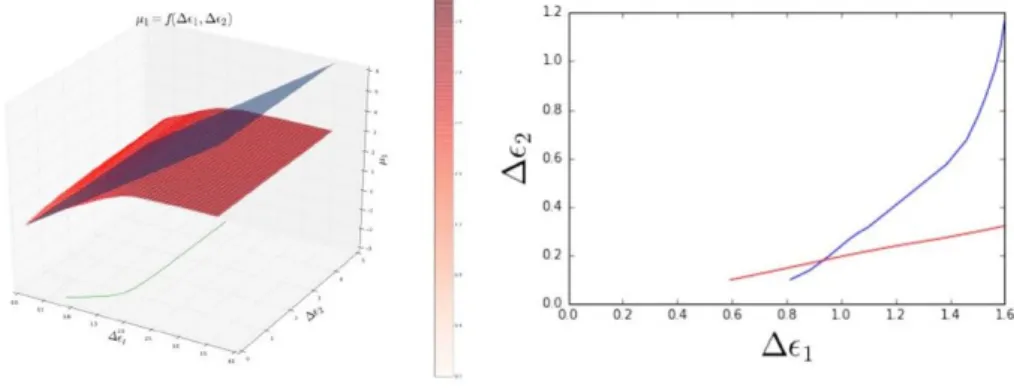
maps µi in the ∆εA, ∆εB. This is illustrated in Figure 3 (left-hand side)

in the F eN i case at equiconcentration, for the F e magnetic moment µF e.

Then, it remains to intersect each of two µi maps (i=F e,i=N i) by the plane

corresponding to the extension of eq. (3b) for the proper value of Ui. This

is illustrated in the same figure for the µF e = 2.8eV , i.e. the value of the

Coulom interaction in pure Fe. We also plot in Figure 3 (left-hand side) the projection of the intersection line in the (∆εF e,∆εNi) layer. Finally, the

equilibrium µA and µB magnetic moments will be given by the common

val-ues of (∆εA, ∆εB) for which there exists simultaneous intersections. This is

achieved by finding the crossing point of the intersection lines projections in the (∆εA, ∆εB) layer. This is illustrated for the F eN i alloy in the right-hand

side of Figure 3, by first keeping for the alloy (as for CoP t) the same values of Ui as in the pure metals (UF e= 2.8 eV, UN i= 2 eV ).

Figure 3: FeNi: left-hand side: Intersecting maps µF e given by the

gener-alization of equation 3a-3b to alloys. The intersection line is projected in (∆εF e, ∆εN i). right-hand side: crossing of the projected intersection lines for

F e and N i.

As can be seen, the single intersection point obtained for (∆εA, ∆εB) =

(0.9 eV, 0.2 eV) leads to the following magnetic moments: µF e = 1.6 µB

and µN i = 0.6 µB, lower that in the pure elements (µF e = 2.2 µB and

µN i = 0.45 µB). However, as in the CoPt case, there is no reason to keep

constant the values of UF e and UN i when going from the pure elements

to the alloy. We have then here again allowed small variations of these Coulomb integrals as a function of the chemical environment, in order to

identify the (∆εA, ∆εB) values which would give values of the equilibrium

magnetic moments consistent with DFT values. One finds that these pro-jections cross for 2.5 eV < UF e < 2.9 eV and 2 eV < UN i < 4 eV . This

gives different 2D (∆εA, ∆εB) intersection lines and therefore different

val-ues of the magnetic moments (µF e, µN i)=f(UF e, UN i) which can be

com-pared to those of the pure elements. From such an analysis, it appears that the case (UF e = 2.9 eV, UN i = 2 eV ) gives values closer to those of

the pure element than those previously determined for the precise values (UF e = 2.8 eV, UN i = 2 eV ), which illustrates the sensibility of the

calcu-lation in this U range. However, if one takes as a reference DFT calcula-tions performed in the L10 phase (µF e = 2.64 µB and µN i = 0.78 µB),[33]

it is more suited to choose the case (UF e = 3 eV, UN i = 2 eV ) which gives

µF e = 2.35 µB and µN i = 0.71 µB. This result indicates that the Coulomb

integral is unchanged for the Ni sites and slightly increased on the Fe ones. Here again, an alternative procedure which either avoids to find the zero of ∆µi, or allows to discriminate between possible multiple solutions if they

exist, is to calculate the magnetic energy balance by a simple extension of the equations(5c)[33]. In that case, the equilibrium magnetic moments

µA,eq(UA, UB) and µB,eq(UA, UB), for a given (UA, UB) couple, are those

cor-responding to the values of (∆εA, ∆εB) for which ∆Eb is minimum.

4

Conclusion

We have presented here a simple way to characterize the variation of the magnetic moment with the environment and to generalize the tight-binding expression of the energy to account for magnetism. This has been illustrated in different systems based on the three ferromagnetic transition elements Co, Fe and Ni. This methodology should be now implemented in the expression of the TB total energy founding numerical simulation in order to account for magnetism effects in complex transition metal compounds including surfaces or more generally including any possible inequivalent sites and defects.

References

[1] J. Friedel: The Physics of Metals, ed. J. M. Ziman (Cambridge Univer-sity Press, 1969), p. 340.

[2] D. Spanjaard, C. Guillot, M.-C. Desjonqu`eres, G. Tr´eglia, J. Lecante, Surf. Sci. Rep. 5 (1985) 1.

[3] S. Sawaya, J. Goniakowski, C. Mottet, A. Sa´ul, G. Tr´eglia, Phys. Rev. B 56 (1997) 12161.

[4] A. Jaafar, C. Goyhenex, G. Tr´eglia, J. Phys.: Condens. Matter 22 (2010) 505503.

[5] L. Zosiak, PhD Thesis, Universit´e de Strasbourg (2013), https://tel.archives-ouvertes.fr/tel-01078044/

[6] C. Goyhenex, G. Tr´eglia, B. Legrand, Surface Science 646 (2016) 261 [7] N. A. Frey, S. Sun: Magnetic Nanoparticle for Information Storage

Ap-plications, in: Inorganic Nanoparticles : Synthesis, ApAp-plications, and Perspectives, Eds. C. Altavilla, E. Ciliberto (2010) CRC Press.

[8] M. V. Lebedeva, V. Pierron-Bohnes, C. Goyhenex, V. Papaefthimiou, S. Zafeiratos, R. R. Nazmutdinov, V. Da Costa, M. Acosta, L. Zosiak, R. Kozubski, D. Muller, E. R. Savinova, Electrochim. Acta 108 (2013) 605.

[9] S. Karoui, H. Amara, B. Legrand, F. Ducastelle, J. Phys.: Condens. Matter 25 (2013) 056005.

[10] M. Sansa, F. Ribeiro, A. Dhouib, G. Tr´eglia, Journal of Physics: Con-densed Matter 28 (2016), 064003

[11] G. Rossi, R. Ferrando, C. Mottet, Nanoalloys: from theory to applica-tion, Faraday Discussions 138 (2008) 193.

[12] O. Ersen, C. Goyhenex, V. Pierron-Bohnes, Phys. Rev. B 78 (2008) 35429.

[13] A. Bieber, F. Gautier, J. Mag. Mag. Mat. 99 (1991) 293.

[14] J. Dorantes-D´avila, H. Dreyss´e, G. Pastor, Phys. Rev. B 55 (1997) 15033.

[15] G. Aut`es, C. Barreteau, D. Spanjaard, M.-C. Desjonsqu`eres, J. Phys.: Condens. Matter 18 (2006) 6785.

[16] C. Barreteau, D. Spanjaard, J. Phys.: Condens. Matter 24 (2012) 406004.

[17] F. Ducastelle, Order and Phase Stability in Alloys, North Holland, 1991. [18] R. Haydock, V. Keine, M. J. Kelly, J. Phys. C 8 (1975) 2592.

[19] G. Tr´eglia, F. Ducastelle, D. Spanjaard, J. de Physique 43 (1982) 341. [20] D.A. Papaconstantopoulos, Handbook of Electronic Structure of

Ele-mental Solids, Plenum, New York, 1986.

[21] C. Goyhenex, G. Trglia, Physical Review B 83 (2011) 075101

[22] C. -S. Yoo, P. S¨oderlind, H. Cynn, J. Phys.: Condens. Matter 10 (1998) L311.

[23] see values reported in : B. I. Min, T. Oguchi, A. J. Freeman, Phys. Rev. B 33 (1986) 7852.

[24] M. Ald´en, S. Mirbt, H. L. Skriver, N. M. Rosengaard, B. Johansson, Phys. Rev. B 46 (1992) 6303.

[25] R.L. Johnston, R. Ferrando, Nanoalloys: from theory to application, Faraday Discussions 138 (2008) 9.

[26] Nanoalloys: Synthesis, Structure and Properties, D. Alloyeau, C. Mot-tet, C. Ricolleau, (Eds), Springer London (2012).

[27] O. Kitakami, H. Sato, Y. Shimada, F. Sato, M. Tanaka, Phys. Rev. B 56 (1997) 13849.

[28] R. Morel,A. Brenac, P. Bayle-Guillemaud, C. Portemont, F. La Rizza, Eur. Phys. J. D 24 (2003) 287.

[29] S. Rives, A. Catherinot, F. Dumas-Bouchiat, C. Champeaux, A. Vide-coq, R. Ferrando, Phys. Rev. B 77 (2008) 085407.

[30] J. M. Soler, E. artacho, J. D. Gale, A. Garcia, J. Junquera, P. Ordejon, D. Sanchez-Portal, J. Phys.: Condens. Matter 14 (2002) 2745.

[31] L. Zosiak, C. Goyhenex, R. Kozubski, G. Tr´eglia, Phys. Rev. B 88 (2013) 014205.

[32] V. Dupuis, G. Khadra, S. Linas, A. Hillion, L. Gragnaniello, A. Tamion, J. Tuaillon-Combes, L. Bardotti, F. Tournus, E. Otero, P. Ohresser, A. Rogalev, F. Wilhelm, J. Mag. Mag. Mat 383 (2015) 73.

[33] M. Sansa, F. Ribeiro, A. Dhouib,N. JaIdane, Tr´eglia, submitted to Phys.