HAL Id: cea-02421719
https://hal-cea.archives-ouvertes.fr/cea-02421719
Submitted on 20 Dec 2019
HAL is a multi-disciplinary open access
archive for the deposit and dissemination of
sci-entific research documents, whether they are
pub-lished or not. The documents may come from
teaching and research institutions in France or
abroad, or from public or private research centers.
L’archive ouverte pluridisciplinaire HAL, est
destinée au dépôt et à la diffusion de documents
scientifiques de niveau recherche, publiés ou non,
émanant des établissements d’enseignement et de
recherche français ou étrangers, des laboratoires
publics ou privés.
Poisson-Box Sampling algorithms for three-dimensional
Markov binary mixtures
A. Zoia, C. Larmier, F. Malvagi, E. Dumonteil, A. Mazzolo
To cite this version:
A. Zoia, C. Larmier, F. Malvagi, E. Dumonteil, A. Mazzolo. Poisson-Box Sampling algorithms for
three-dimensional Markov binary mixtures. Journal of Quantitative Spectroscopy and Radiative
Transfer, Elsevier, 2018, 206, pp.70-82. �10.1016/j.jqsrt.2017.10.020�. �cea-02421719�
Poisson-Box Sampling algorithms for three-dimensional Markov binary mixtures
Coline Larmiera, Andrea Zoiaa,∗, Fausto Malvagia, Eric Dumonteilb, Alain Mazzoloa
aDen-Service d’Etudes des R´eacteurs et de Math´ematiques Appliqu´ees (SERMA), CEA, Universit´e Paris-Saclay, 91191 Gif-sur-Yvette, FRANCE. bIRSN, 31 Avenue de la Division Leclerc, 92260 Fontenay aux Roses, FRANCE.
Abstract
Particle transport in Markov mixtures can be addressed by the so-called Chord Length Sampling (CLS) methods, a family of Monte Carlo algorithms taking into account the effects of stochastic media on particle propagation by generating on-the-fly the material interfaces crossed by the random walkers during their trajectories. Such methods enable a significant reduction of computational resources as opposed to reference solutions obtained by solving the Boltzmann equation for a large number of realizations of random media. CLS solutions, which neglect correlations induced by the spatial disorder, are faster albeit approximate, and might thus show discrepancies with respect to reference solutions. In this work we propose a new family of algorithms (called ’Poisson Box Sampling’, PBS) aimed at improving the accuracy of the CLS approach for transport in d-dimensional binary Markov mixtures. In order to probe the features of PBS methods, we will focus on three-dimensional Markov media and revisit the benchmark problem originally proposed by Adams, Larsen and Pomraning Adams et al. (1989) and extended by Brantley Brantley (2011): for these configurations we will compare reference solutions, standard CLS solutions and the new PBS solutions for scalar particle flux, transmission and reflection coefficients. PBS will be shown to perform better than CLS at the expense of a reasonable increase in computational time.
Keywords: Chord Length Sampling, Markov geometries, Poisson, Box, benchmark, Monte Carlo, Tripoli-4 R
1. Introduction
Linear particle transport theory in random media is key to several applications in nuclear science and engineering, such as neutron diffusion in pebble-bed reactors or randomly mixed water-vapour phases in boiling water reactors Pomraning (1991); Larsen and Vasques (2011); Levermore et al. (1986); Sanchez (1986); Levermore et al. (1988), and inertial con-finement fusion Zimmerman (1990); Zimmerman and Adams (1991); Haran et al. (2000). Material and life sciences as well as radiative transport also often involve particle propagation in random media Torquato (2002); Barthelemy et al. (2009); Davis and Marshak (2004); Kostinski and Shaw (2001); Malvagi et al. (1992); Tuchin (2007); Brantley et al. (2017).
In this context, the material cross sections composing the tra-versed medium and the particle sources are distributed accord-ing to some statistical laws, and the physical observable of in-terest is typically the ensemble-averaged angular particle flux hϕ(r, ω)i, namely,
hϕ(r, ω)i = Z
P(q)ϕ(q)(r, ω)dq, (1)
where ϕ(q)(r, ω) satisfies the linear Boltzmann equation
cor-responding to a single realization q, and P(q) is the station-ary probability of observing the state q for the material cross sections and/or the sources Pomraning (1991); Zuchuat et al.
(1994). In the following, we consider linear particle transport in binary stochastic mixing composed of two immiscible ran-dom media (say α and β).
Exact solutions for hϕi, or more generally for some ensemble-averaged functional hF[ϕ]i of the particle flux, can be obtained using a so-called quenched disorder approach: an ensemble of medium realizations are first sampled from the un-derlying mixing statistics; then, the linear transport equation is solved for each realization by either deterministic or Monte Carlo methods, and the physical observables of interest F[ϕ] are determined; ensemble averages are finally computed. In a series of recent papers, we have provided reference solutions for particle transport in d-dimensional random media with Markov statistics Larmier et al. (2017a,b), where the spatial disorder has been generated by means of homogeneous and isotropic d-dimensional Poisson tessellations Larmier et al. (2016).
Reference solutions for particle transport in stochastic me-dia are computationally expensive, so faster but approximate methods have been therefore proposed. A first approximate approach consists in deriving an expression for the ensemble-averaged flux hϕi in each material: this generally leads to an infinite hierarchy of equations, which ultimately requires a clo-sure formula, such as in the celebrated Levermore-Pomraning model Pomraning (1991); Levermore et al. (1986); Su and Pom-raning (1995). A second approach is based on Monte Carlo algorithms that reproduce the ensemble-averaged solutions to various degrees of accuracy by modifying the displacement laws of the simulated particles in order to take into account the effects of spatial disorder Zimmerman and Adams (1991);
Donovan et al. (2003); Donovan and Danon (2003). The Chord Length Sampling (CLS) algorithm is perhaps the most repre-sentative and best-known example of such algorithms: the ba-sic idea behind CLS is that the interfaces between the con-stituents of the stochastic medium are sampled on-the-fly dur-ing the particle displacements by drawdur-ing the distances to the following material boundaries from a distribution depending on the mixing statistics. It has been shown that the CLS algorithm formally solves the Levermore-Pomraning model for Marko-vian binary mixing Zimmerman and Adams (1991); Sahni (1989a,b). The free parameters of the CLS model are the av-erage chord length Λi through each material, and the volume
fraction pi. Since the spatial configuration seen by each
parti-cle is regenerated at each partiparti-cle flight, the CLS corresponds to an annealed disorder model, as opposed to the quenched disor-der of the reference solutions, where the spatial configuration is frozen for all the traversing particles. This means that the cor-relations on particle trajectories induced by the spatial disorder are neglected in the standard implementation of CLS. General-ization of these Monte Carlo algorithms including partial mem-ory effects due to correlations for particles crossing back and forth the same materials have been also proposed Zimmerman and Adams (1991).
CLS, which had been originally formulated for Markov statistics, has been extensively applied also to randomly dis-persed spherical inclusions into background matrices, with ap-plication to pebble-bed and very high temperature gas-cooled reactors Donovan et al. (2003); Donovan and Danon (2003). In order to quantify the accuracy of CLS with respect to ref-erence solutions for spherical inclusions, several comparisons have been proposed in two and three dimensions Donovan et al. (2003); Donovan and Danon (2003); Brantley and Martos (2011); Brantley (2014). Some methods to mitigate the errors between CLS and the reference solutions have been presented in the context of eigenvalue calculations, e.g., in Liang et al. (2013). For Markov mixing specifically, a number of bench-mark problems comparing CLS and reference solutions have been proposed in the literature so far Adams et al. (1989); Brantley (2011); Zuchuat et al. (1994); Brantley and Palmer (2009); Brantley (2009) with focus on 1d-geometries (either of the rod or slab type); flat 2d geometries have been considered in Haran et al. (2000). These benchmark comparisons have been recently extended to d-dimensional Markov geometries, for d= 2 (extruded) and d = 3 Larmier et al. (2017d).
Not surprisingly, CLS solutions may display discrepancies as compared to reference solutions, whose relevance varies strongly with the system dimensionality, the average chord length and the material volume fraction Larmier et al. (2017d). For the case of 1d slab geometries with Markov mixing, pos-sible improvements to the standard CLS algorithm accounting for partial memory effects for particle trajectories have been de-tailed Zimmerman and Adams (1991), and numerical tests have revealed that these corrections contribute to palliating the dis-crepancies Brantley (2011), although a generalization to higher dimensions seems hardly feasible with reasonable computa-tional burden Zimmerman and Adams (1991).
In this work we propose a new family of Monte Carlo
algo-rithms aimed at improving the standard CLS for d-dimensional Markov media, yet keeping the increase in algorithmic com-plexity to a minimum. Inspiration comes from the obser-vation that the physical observables related to particle trans-port through quasi-isotropic Poisson tessellations based on Cartesian boxes are almost identical to those computed for isotropic Poisson tessellations, for any dimension d Larmier et al. (2017b,c), which confirms the considerations in Ambos and Mikhailov (2011). This quite remarkable property suggests that the standard CLS algorithm can be extended by replacing the memoryless sampling of material interfaces by the sampling of d-dimensional Cartesian boxes sharing the statistical features of quasi-isotropic Poisson tessellations, so as to mimic the spa-tial correlations that would be induced by isotropic Poisson tes-sellations. We will call this class of algorithms Poisson Box Sampling (PBS).
In order to illustrate the behaviour of the PBS with re-spect reference solutions and to CLS, we will revisit the clas-sical benchmark problem for transport in Markov binary mix-tures proposed by Adams, Larsen and Pomraning Adams et al. (1989) and revisited by Brantley Brantley (2011). The physical observables of interest will be the particle flux hϕi, the trans-mission coefficient hTi and the reflection coefficient hRi, for incident flux conditions and for uniform interior sources.
This paper is organized as follows: in Sec. 2 we will recall the benchmark specifications that will be used for our analy-sis in dimension d = 3. In Sec. 3 we will illustrate the ref-erence solutions for the benchmark problem obtained by using isotropic and quasi-isotropic Poisson tessellations: this prelim-inary investigation will allow establishing that quasi-isotropic tessellations yield results very close to those of isotropic tessel-lations, as expected based on previous investigations. Then, in Sec. 4 we will describe in detail the PBS algorithms, compare these methods to the reference solutions and to the standard CLS approach, and discuss their respective merits and draw-backs. Conclusions will be finally drawn in Sec. 5.
2. Benchmark specifications
In order for this paper to be self-contained, we briefly recall here the benchmark specifications that have been selected for this work, which are essentially drawn from those originally proposed in Adams et al. (1989) and Zuchuat et al. (1994), and later extended in Brantley (2011); Brantley and Palmer (2009); Brantley (2009).
We consider mono-kinetic linear particle transport through a stochastic binary medium with homogeneous and isotropic Markov mixing. The medium is non-multiplying, with isotropic scattering. The geometry consists of a cubic box of side L= 10 (in arbitrary units), with reflective boundary conditions on all sides of the box except two opposite faces (say those perpen-dicular to the x axis), where leakage boundary conditions are imposed. Two kinds of sources will be considered: either an imposed normalized incident angular flux on the leakage sur-face at x = 0 (with zero interior sources), or a distributed ho-mogeneous and isotropic normalized interior source (with zero incident angular flux on the leakage surfaces). The benchmark
configurations pertaining to the former kind of source will be called suite I, whereas those pertaining to the latter will be called suite II Brantley (2011). Markov mixing statistics are entirely defined by assigning the average chord length for each material i = α, β, namely Λi. The (homogeneous) probability
piof finding material i at an arbitrary location within the box
follows from
pi=
Λi
Λi+ Λj
. (2)
By definition, the material probability piyields the volume
frac-tion for material i. The cross secfrac-tions for each material will be denoted as customaryΣifor the total cross section andΣs,i
for the scattering cross section. The average number of par-ticles surviving a collision in material i will be denoted by ci = Σs,i/Σi ≤ 1. The physical parameters for the benchmark
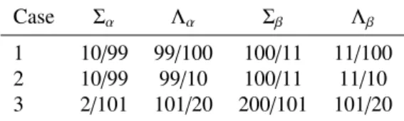
configurations are recalled in Tabs. 1 and 2: the benchmark specifications include three cases (numbered 1, 2 and 3, cor-responding to different materials), and three sub-cases (noted a, b and c, corresponding to different cifor a given material) for
each case Adams et al. (1989).
Case Σα Λα Σβ Λβ
1 10/99 99/100 100/11 11/100 2 10/99 99/10 100/11 11/10 3 2/101 101/20 200/101 101/20
Table 1: Material parameters for the three cases of the benchmark configura-tions.
Sub-case a b c cα 0 1 0.9
cβ 1 0 0.9
Table 2: Scattering probabilities for the three sub-cases of the benchmark con-figurations.
Following Brantley (2011), the physical observables of in-terest for the benchmark will be the ensemble-averaged out-going particle currents hJi on the two surfaces with leakage boundary conditions, the ensemble-averaged scalar particle flux hϕ(x)i = hR R R ϕ(r, ω)dωdydzi along 0 ≤ x ≤ L, and the total scalar flux hϕi= hR ϕ(x)dxi. For the suite I configurations, the outgoing particle current on the side opposite to the imposed current source represents the ensemble-averaged transmission coefficient, namely, hTi = hJx=Li, whereas the outgoing
par-ticle current on the side of the current source represents the ensemble-averaged reflection coefficient, namely, hRi = hJx=0i.
For the suite II configurations, the outgoing currents on oppo-site faces are expected to be equal (within statistical fluctua-tions), for symmetry reasons. In this case, we also introduce the average leakage current hLi= h(T + R)/2i.
3. Reference solutions
In view of computing reference solutions for particle trans-port in three-dimensional quenched disorder, the generation of Markov mixing statistics will be based on random tessellations, which are stochastic aggregates of disjoint and space-filling cells obeying a given probability distribution Santalo (1976). In the following we will describe the two kinds of stochastic geometries that will be used for our analysis, namely isotropic Poisson tessellations and quasi-isotropic Poisson tessellations. Reference solutions for a d-dimensional generalization of the Adams, Larsen and Pomraning benchmark with homogeneous and isotropic Markov mixing have been thoroughly described in Larmier et al. (2017a), where the ensemble-averaged scalar particle flux hϕ(x)i and the currents hRi and hT i have been de-termined. In this section we recall the methods and the key results, and detail the changes and the additions that have been made with respect to our previous work.
3.1. Isotropic Poisson tessellations
Three-dimensional homogeneous and isotropic Poisson tes-sellations are obtained by partitioning an arbitrary domain with random planes sampled from an auxiliary Poisson process San-talo (1976); Miles (1964, 1972). A single free parameter ρP
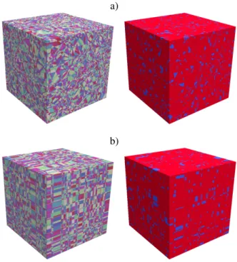
(which is called the tessellation density) is required, which for-mally corresponds to the average number of planes of the tes-sellation that would be intersected by an arbitrary segment of unit length. An explicit construction amenable to Monte Carlo realizations for 2d geometries of finite size had been established in Switzer (1964) (for a numerical investigation see, e.g., Ha-ran et al. (2000); Lepage at al. (2011)), and recently generalized to d-dimensional domains Ambos and Mikhailov (2011). The algorithm for 3d tessellations of a cube of side L has been de-tailed in Larmier et al. (2016). An example of realization of homogeneous and isotropic Poisson tessellation is provided in Fig. 1.
Isotropic Poisson geometries satisfy a Markov property: for domains of infinite size, arbitrary lines drawn through the tes-sellation will be cut by the surfaces of the polyhedra into seg-ments whose lengths ` are exponentially distributed, with av-erage chord length h`i = 1/ρP Santalo (1976). The quantity
Λ = h`i intuitively defines the correlation length of the Poisson geometry, i.e, the typical linear size of a polyhedron composing the random tessellation Pomraning (1991).
3.2. Colored stochastic geometries
Homogeneous and isotropic binary Markov mixtures re-quired for the reference solutions corresponding to the bench-mark specifications are obtained as follows: first, an isotropic Poisson tessellation is constructed as described above. Then, each polyhedron of the geometry is assigned a material compo-sition by formally attributing a distinct ‘color’ α or β, with as-sociated complementary probabilities pαand pβ= 1 − pα
Pom-raning (1991). This gives rise to (generally) non-convex α and β clusters, each composed of a random number of convex poly-hedra. An example of realization for a colored Poisson tessel-lation is shown in Fig. 1.
The average chord lengthΛαthrough clusters with composi-tion α is related to the correlacomposi-tion lengthΛ of the geometry via Λ = (1 − pα)Λα, and forΛβwe similarly haveΛ = pαΛβ. This yields 1/Λα+ 1/Λβ= 1/Λ, and we recover
pα = Λ
Λβ =
Λα
Λα+ Λβ. (3)
Based on the formulas above, and using ρP = 1/Λ, the
param-eters of the colored Poisson geometries corresponding to the benchmark specifications provided in Tab. 1 are easily derived.
3.3. Poisson-Box tessellations
Box tessellations refer to a class of anisotropic stochastic ge-ometries composed of Cartesian parallelepipeds with random sides Santalo (1976). The special case of Poisson-Box tessel-lations was proposed in Miles (1972): a domain is partitioned by randomly generated planes orthogonal to the three axes x, y and z through a Poisson process of intensity ρx, ρyand ρz,
re-spectively. We will assume that the three parameters are equal, namely, ρx= ρy= ρz= ρB, which leads to homogeneous
quasi-isotropic Poisson tessellations of density ρB.
The explicit construction for Poisson-Box tessellations re-stricted to a cubic box of side L has been provided in Larmier et al. (2017b). An example of realization of Poisson-Box tessel-lation is illustrated in Fig. 1. The chord distribution through Poisson-Box tessellations is not exponential; its average can be computed exactly, and yields Λ = (2/3)/ρBMiles (1972);
Larmier et al. (2017b). The coloring procedure is identical to that of isotropic Poisson tessellations, and the properties of the average chord lengths through colored clusters carry over as they stand: an example of colored realization is shown in Fig. 1. In order to avoid confusion with the Poisson tessellations de-scribed above, we will refer to Poisson-Box geometries simply as Box tessellations in the following.
3.4. Comparing Poisson and Box tessellations
In a series of benchmark calculations for multiplying and non-multiplying systems we have shown by Monte Carlo simu-lations that Box tesselsimu-lations yield physical observables related to particle transport that are very close to those computed for isotropic Poisson tessellations Larmier et al. (2017b,c), which confirms the findings in Ambos and Mikhailov (2011). Since this property represents a crucial step towards the construction of the PBS algorithms that will be presented in Sec. 4, we would like to preliminarily verify that this peculiar feature carries over to the Adam, Larsen and Pomraning benchmark configurations. The key point is that both tessellations depend on a single free parameter, namely the average chord lengthΛ, in addition to the coloring probability p. For isotropic Markovian binary mixtures, the average chord length of the Poisson tessellation and the coloring probability are chosen so that the resulting av-erage chord lengths in the colored clusters, namelyΛαandΛβ,
match the correlation lengths in the random media Pomraning (1991).
A natural choice is therefore to set Λα andΛβ to be equal for Poisson and Box tessellations, which ensures that the two
a)
b)
Figure 1: Examples of realizations of a) homogeneous isotropic Poisson tessel-lations b) homogeneous Box tesseltessel-lations, corresponding to the Case 1 of the benchmark specifications (Λα= 99/100, Λβ= 11/100), before (left) and after
(right) attributing the material label, with probability p= 0.9 of assigning the label α. Red corresponds to the label α and blue to the label β. The size of the cube is L= 10.
colored geometries are ‘statistically equivalent’. As shown in Larmier et al. (2017b), this can be achieved by choosing the same parametersΛ and p for the two tessellations. Correspond-ingly, we have a constraint on the tessellation densities ρPand
ρB, which must now satisfy
1
Λ = ρP=
3
2ρB. (4)
Numerical simulations show that by imposing Eq. (4) the chord length distributions for the two tessellations are barely distin-guishable Larmier et al. (2017b,c), which is of utmost impor-tance since the properties of particle transport through random media mostly depend on the shape of the chord length distribu-tion Pomraning (1991).
The similarity of the chord length distributions is all the more striking when considering that other geometrical features do not share comparable affinities. For instance, if we set the average chord lengthΛ to be equal for the two tessellations as in Eq. (4), the average volumes of a typical polyhedron read
hViP= 6 π Λ 3 (5) hViB= 3 2 !3 Λ3, (6)
respectively, i.e., the average volume of the Box tessellations is much larger than that of the Poisson tessellations Larmier et al. (2017b).
3.5. Simulation results for reference solutions
For each benchmark configuration, a large number M of ge-ometries has been generated, and the material properties have been attributed to each volume as described in Larmier et al. (2017a). Then, for each realization k of the ensemble, lin-ear particle transport has been simulated by using the produc-tion Monte Carlo code Tripoli-4 R, developed at CEA Brun et
al. (2015). Tripoli-4 R is a general-purpose stochastic
trans-port code capable of simulating the propagation of neutral and charged particles with continuous-energy cross sections in arbi-trary geometries. In order to comply with the benchmark spec-ifications, constant cross sections adapted to mono-energetic transport and isotropic angular scattering have been prepared. The number of simulated particle histories per configuration is 106. For a given physical observable O, the benchmark solution is obtained as the ensemble average
hOi= 1 M M X k=1 Ok, (7)
where Okis the Monte Carlo estimate for the observable O
ob-tained for the k-th realization. Specifically, currents Rkand Tkat
a given surface are estimated by summing the statistical weights of the particles crossing that surface. Scalar fluxes ϕk(x) have
been tallied using the standard track length estimator over a pre-defined spatial grid containing 102 uniformly spaced meshes
along the x axis.
The error affecting the average observable hOi results from two separate contributions, the dispersion
σ2 G= 1 M M X k=1 Ok2− hOi2 (8)
of the observables exclusively due to the stochastic nature of the geometries and of the material compositions, and
σ2 O= 1 M M X k=1 σ2 Ok, (9)
which is an estimate of the variance due to the stochastic nature of the Monte Carlo method for particle transport, σ2
Ok being the
dispersion of a single calculation Donovan and Danon (2003); Donovan et al. (2003). The statistical error on hOi is then esti-mated as σ[hOi] = s σ2 G M + σ 2 O. (10)
The reference solutions corresponding to isotropic Poisson tessellations have been first presented in Larmier et al. (2017a) with M = 103 realizations for every benchmark configuration.
In order to reduce the dispersion of the observables due to the statistical nature of the geometries, a new set of reference solu-tions has been computed in Larmier et al. (2017d) by increas-ing the number of realizations for the benchmark configura-tions displaying larger correlation lengths (i.e., larger material chunks). The data for reference solutions presented here are taken from Larmier et al. (2017d): we have set M = 2 × 10⁴
for the sub-case 2b of the suite II; M= 5 × 10³for all the other sub-cases of case 2; M= 5×10⁴for the sub-case 3b of the suite II; and M = 104 for all the other sub-cases of case 3. For all remaining cases and sub-cases, we have used the same number of realizations as in Larmier et al. (2017a), namely, M = 103.
Additionally, reference solutions corresponding to Box tessella-tions have been computed for each benchmark configuration by following the same procedure as above, and the number of real-izations has been set equal to that of the corresponding Poisson tessellations.
Particle transport calculations have been run on a cluster based at CEA, with Intel Xeon E5-2680 V2 2.8 GHz proces-sors. For the simulations discussed here considerable speed-ups have been obtained for the most fragmented geometries thanks to the possibility of reading pre-computed connectivity maps for the volumes composing the geometry, which largely increases the performances of particle tracking.
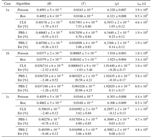
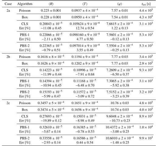
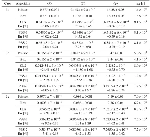
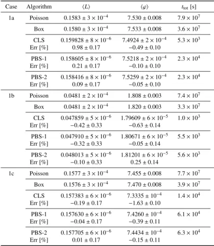
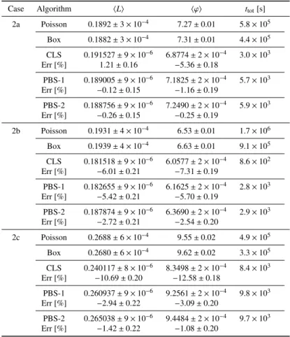
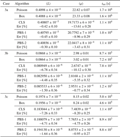
Reference solutions for both tessellations are provided in Tabs. 3 to 5 for the benchmark cases corresponding to suite I, and in Tabs. 6 to 8 for the benchmark cases corresponding to suite II, respectively: the ensemble-averaged total scalar flux hϕi, transmission coefficient hTi, and reflection coefficient hRi are displayed for Poisson and Box tessellations. The respec-tive computer times are also provided in the same tables. The ensemble-averaged spatial flux hϕ(x)i is illustrated in Figs. 2 to 4. As mentioned above, the reference solutions for Poisson ge-ometries are taken from reference Larmier et al. (2017d); the reference solutions for Box tessellations have never been pre-sented before.
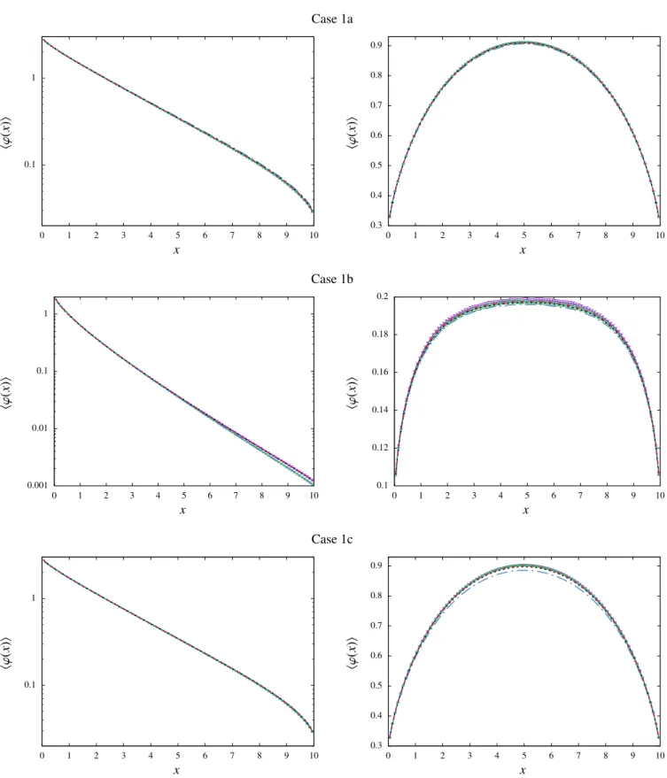
Simulation results for the Adam, Larsen and Pomraning benchmark configurations basically confirm our previous find-ings: the physical observables related to particle transport through Box tessellations are very close to those of isotropic Poisson tessellations, which was expected based on their re-spective chord length distributions being very similar. The agreement between the two sets of results increases by decreas-ing the average chord length (i.e., for more fragmented tessella-tions). An exception must be remarked for sub-case 1b of suite I, in particular for the transmission coefficient hTi, despite this configuration being highly fragmented. Since this sub-case is composed of absorbing chunks dispersed in a scattering back-ground, the observed discrepancy might be attributed to the ef-fects induced by the shape of the chunks on particle transport (which are different for the two tessellations, as noticed above). For the spatial flux profiles, slight differences emerge for the less fragmented configurations, e.g., sub-cases 2b, 3a and 3b of suiteI.
The computer time required for the reference solutions (as shown in Tabs. 3 to 5) depends on the material compositions and increases with the complexity of the configurations, i.e., with the number of polyhedra composing the tessellation. For a given average chord length Λ, the average number of vol-umes is smaller in Box geometries than in Poisson geometries, which follows from the expressions of the typical volumes in Eq. (6). Transport simulations in Box tessellations are faster than in Poisson tessellations for configurations composed of a large number of polyhedra, such as those of case 1; for cases 2
and 3, finite-size effects due to Λ being comparable to L come into play, and computer times become almost identical for Pois-son and Box geometries.
4. Approximate solutions: from CLS to PBS
Reference solutions based on the quenched disorder ap-proach are very demanding in terms of computational re-sources, so that intensive research efforts have been devoted to the development of Monte Carlo-based annealed disorder mod-els capable of approximating the effects of spatial disorder on-the-fly during particle trajectories, i.e., within a single transport simulation. In this section we first briefly recall the standard CLS algorithm, for the sake of completeness, and then intro-duce a new class of Monte Carlo methods, called Poisson Box Sampling (PBS), combining the principles of CLS with the gen-eration of material volumes inspired by the findings concerning Box tessellations. Simulation results of the PBS for the bench-mark configurations will be compared to those of CLS and to the reference solutions obtained above.
4.1. Chord Length Sampling (CLS)
The annealed disorder algorithms initially developed by Zimmerman and Adams go now under the name of Chord Length Sampling methods Zimmerman (1990); Zimmerman and Adams (1991). The standard form of CLS (Algo-rithm A in Zimmerman and Adams (1991)) formally solves the Levermore-Pomraning equations corresponding to Markov mixing with the approximation that memory of the crossed ma-terial interfaces is lost at each particle flight Sahni (1989a,b). Algorithm A has the following structure Zimmerman and Adams (1991):
• Step 1: each particle history begins by sampling position, angle and velocity from the specified source, as custom-ary. Moreover, the particle is assigned a supplementary attribute, the material label, which is sampled according to the volume fraction probability pi.
• Step 2: three distances are computed: the distance `bto the
next physical boundary, along the current direction of the particle; the distance `cto collision, which is determined
by using the material cross section chosen at the previous step: if the particle has a material label α, e.g., then `c
will be drawn from an exponential distribution of param-eter 1/Σα; and the distance `ito material interface, which
is sampled from an exponential distribution with parame-terΛα, i.e., the average chord length of material α, if the particle has a material label α (whence the name of CLS).
• Step 3: the minimum distance among `b, `cand `i has to
be selected. If the minimum is `b, the particle is moved
along a straight line until the external boundary is hit (the direction is updated in the case of reflection); if the mini-mum is `c, the particle is moved to the collision point, and
the outgoing particle features are selected according to the collision kernel pertaining to the current material label; if
the minimum is `i, the particle is moved to the interface
be-tween the two materials, and the material label is switched. If the particle has not been absorbed, return to Step 2.
The particle will ultimately either get absorbed in one of the chunks or leak out of the boundaries of the random medium. As observed above, Algorithm A assumes that the particle has no memory of its past history, and in particular the crossed interfaces are immediately forgotten (which is consistent with the closure formula of the Levermore-Pomraning model). In this respect, CLS is an approximation of the exact treatment of disorder-induced spatial correlations. In particular, CLS is expected to be less accurate in the presence of strong scatter-ers with optically thick mean material chunk length Brantley (2011); Larmier et al. (2017d). A thorough discussion of the shortcomings of the CLS approach for d= 1 can be found, e.g., in Liang and Ji (2011).
4.2. Poisson Box Sampling (PBS)
For the case of 1d slab geometries, two improved versions of CLS Algorithm A have been proposed in the literature, by partially taking into account the memory effects induced by the spatial correlations Zimmerman and Adams (1991): in the for-mer, called Algorithm B, instead of sampling the material inter-faces one at a time a full random slab is generated, and particles do not switch material properties until either the forward or the backward surfaces of the slab are crossed; in the latter, called Algorithm C, a slab is generated as in Algorithm B, and the slab traversed before entering the current one is also kept in mem-ory. The basic idea behind Algorithms B and C is to preserve the shape and the position of the material chunks (thus partially restoring spatial correlations) by generating an additional typi-cal random slab whenever particles cross the material surfaces of the current volume.
As expected, Algorithms B and C have been shown to ap-proximate the reference solutions for Markov mixing in 1d more accurately than Algorithm A, at the expense of an in-creased computational cost Brantley (2011); Zimmerman and Adams (1991). Algorithm B in particular has been extensively tested for the Adams, Larsen and Pomraning benchmark in slab geometries, and performs better than Algorithm A for all con-figurations Brantley (2011). As observed in Zimmerman and Adams (1991), it is not trivial to extend Algorithms B and C to higher dimensions: this can be immediately understood by remarking that randomly generating a typical material chunk in dimension three with Markov mixing would correspond to sam-pling a typical polyhedral cell of the isotropic Poisson tessella-tions, whose exact distributions for the volume, surface, num-ber of faces, etc., are unfortunately unknown to this day Miles (1972); Santalo (1976); Larmier et al. (2016). In dimension one the typical chunk is a slab of exponentially distributed width, which considerably simplifies the computational burden.
A possible way to overcome this issue and improve Algo-rithm A in higher dimensions is however suggested by the nu-merical findings concerning Box tessellations. Since the chord length distribution of Box tessellations is very close to that of Poisson tessellations, it seems reasonable to extend Algorithm
B by generating on-the-fly the typical cells of Box tessellations, i.e., Cartesian boxes with exponentially distributed side lengths. The generalization of Algorithm C would immediately follow by keeping memory of the last visited box. We will call this new class of Monte Carlo algorithms Poisson Box Sampling (PBS), and we will denote by PBS-1 the former (inspired by Algo-rithm B) and by PBS the latter (inspired by AlgoAlgo-rithm C). In view of the aforementioned similarity between quasi-isotropic and isotropic Poisson tessellations, intuitively we expect that PBS methods will preserve the increased accuracy of Algo-rithms B and C over Algorithm A, yet allowing for a relatively straightforward construction and a fairly minor additional com-putational burden.
By adapting the strategy of CLS, the algorithm for PBS-1 proceeds as follows:
• Step 1: initialize each particle history by sampling posi-tion, angle and velocity from the specified source. In addi-tion, a random Cartesian box is generated. The box is de-fined by its material label i and its spatial position, given by the coordinates (xc, yc, zc) of its center and its sides:
lx, ly and lz. Three pairs of random numbers, namely,
(∆+x, ∆−x), (∆+y, ∆−y) and (∆+z, ∆−z), are sampled from inde-pendent exponential distributions of average 3Λ/2. For suite I, we do not sample the value of ∆−x, and we set
∆−
x = 0. Then, we set the center of the box
xc= x + (∆+x−∆ − x)/2, (11) yc= y + (∆+y −∆ − y)/2, (12) zc= z + (∆+z −∆ − z)/2, (13)
and the sides
lx= ∆+x+ ∆ − x, (14) ly= ∆+y+ ∆ − x, (15) lz= ∆+z + ∆ − z. (16)
The material label of the box is sampled according to pi.
• Step 2: we compute three distances: the distance `bto the
next physical boundary, along the current direction of the particle; the distance `cto collision, which is determined
by using the material cross section that has been chosen at the previous step: if the particle is in a box with material label α, e.g., then `c will be drawn from an exponential
distribution of parameter 1/Σα; and the distance `ito the
next interface of the current box along the particle direc-tion (the boundaries of the box being easily determined).
• Step 3: the minimum distance among `b, `cand `i has to
be selected: if the minimum is `b, the particle is moved
along a straight line until the external boundary is hit (the direction is updated in the case of reflection); if the mini-mum is `c, the particle is moved to the collision point, and
the outgoing particle features are selected according to the collision kernel pertaining to the current material label; if the minimum is `i, the particle is moved along a straight
line until the interface of the current box is hit: a new box
is sampled as detailed below, and the new box becomes the current box. If the particle has not undergone a cap-ture, return to Step 2.
For the sampling of a new box at Step 3, we begin by draw-ing a random spacdraw-ing δ from an exponential distribution with average 3Λ/2. Without loss of generality, if the interface of the current box hit by the particle is perpendicular to the x-axis, we set the following values for the side lxof the new box and the
position xcof its center: lx= δ, xc= x + lxωx/|ωx|, where ωx
is the particle direction along the x-axis. The other features of the current box, namely, ly, lz, ycand zc, are left unchanged for
the new box (as suggested by the construction of Box tessella-tions). We would proceed in the same way for the y- and z-axis. Finally, the label of the new box is randomly sampled according to the coloring probability pi.
Contrary to Algorithm A, the correlations induced by spatial disorder are partially preserved by the PBS-1 algorithm: in-deed, each particle will see the same material properties until the current box is left. Moreover, when a new box is created, its features strongly depend on those of the previous box. This should globally improve the accuracy of PBS-1 with respect to CLS in reproducing the reference solutions for the bench-mark. Long-range correlations spanning more than a box (i.e., a linear size of the order ofΛ) are nonetheless suppressed, so that we still expect some discrepancies between PBS-1 solu-tions and those obtained by the quenched disorder approach for either Poisson or Box tessellations.
In order to further improve the accuracy of the PBS methods, we propose a second method, inspired by Algorithm C, that will be denoted PBS-2. The strategy is exactly as in the PBS-1 al-gorithm, the only difference being in the fact that, once a new box has been sampled, the old box is not deleted but is kept in memory (size, position and material label) until a new ma-terial interface is selected. If the particle leaves the new box by another interface, the old box is definitively deleted, another box is sampled and the new box becomes the old box. If the selected interface is the one that has been kept in memory, the new box will simply be the old box, and the roles are reversed. This implementation intuitively extends the range of spatial cor-relations, and is thus supposed to correspondingly enhance the accuracy with respect to reference solutions, at the expense of increasing the computational burden, too.
4.3. Simulation results
The simulation results corresponding to CLS and PBS for the total scalar flux hϕi, the transmission coefficient hTi and the reflection coefficient hRi are provided in Tabs. 3 to 5 for the benchmark cases corresponding to suite I, and in Tabs. 6 to 8 for the benchmark cases corresponding to suite II, respectively. The spatial flux hϕ(x)i is illustrated in Figs. 2 to 4. For the CLS and PBS simulations of the benchmark configurations we have used 109particles (103replicas with 106particles per replica),
with resulting statistical uncertainties associated to each phys-ical observable O denoted by σCLS[O] and σPBS[O],
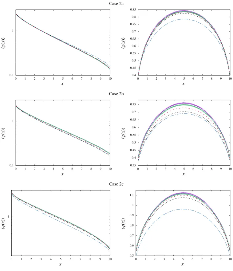
Generally speaking, the solutions computed with PBS-1 show a better agreement with respect to the reference solutions based on Poisson tessellations than those computed with CLS, and overall remarkably well approximate the benchmark ob-servables. Moreover, as expected from the previous consider-ations, PBS-2 shows a further enhanced accuracy with respect to PBS-1. A single exception has been detected for sub-case 1b of suite I, as reported in Tab. 3 and in Fig. 2. For this con-figuration, the results of the Box tessellations are slightly dif-ferent from those of Poisson tessellations, as observed above, for the spatial flux and the transmission coefficient. It turns out that both PBS algorithms provide results that are in excellent agreement with the reference solutions for the Box tessellation, which is consistent with their implementation. However, be-cause of the observed discrepancy between Box and Poisson tessellations for sub-case 1b, PBS show a small bias with re-spect to Poisson reference solutions. For the same case, CLS displays a better accuracy as compared to Poisson solutions, and this is most probably due to the fact that this algorithm ex-actly preserves isotropy.
The analysis of the approximate solutions suggests that the accuracy of CLS globally improves when decreasing the aver-age chord lengthΛ: configurations pertaining to case 1 globally show a better agreement than those of case 2, and those of case 2 show a better agreement than those of case 3, as pointed out in Larmier et al. (2017d). The improved PBS methods are less sensitive to the average chord lengthΛ and show a satisfactory agreement for all benchmark configurations.
Computer times for the CLS and PBS solutions are also pro-vided in Tabs. 3 to 5: not surprisingly, the approaches based on annealed disorder are much faster than the reference methods, since a single transport simulation is needed. PBS methods, while still much faster than reference solutions, for most con-figurations take sensibly longer than CLS: this is partly due to the increased complexity of the algorithms, and partly due to the fact that CLS is based on the sampling of the colored chord lengths (corresponding to clusters of polyhedra sharing all the same material label), whereas PBS require the sampling of un-colored boxes one at a time. Nonetheless, keeping in memory a further box amounts to an almost negligible additional compu-tational burden for PBS-2 as opposed to PBS-1.
5. Conclusions
In this paper we have proposed a new family of Monte Carlo methods aimed at approximating ensemble-averaged observ-ables for particle transport in Markov binary mixtures, where reference results are obtained by sampling medium realizations from homogeneous and isotropic Poisson tessellations. The so-called Algorithm A of Chord Length Sampling method is per-haps the most widely adopted simulation tool to provide such approximate solutions, based on the Levermore-Pomraning model. Several numerical investigations have shown that Al-gorithm A works reasonably well in most cases, yet discrep-ancies between CLS and reference solutions may appear due to the fact that Algorithm A neglects the correlations induced
by spatial disorder. For the case of one-dimensional slab ge-ometries, two variants of the standard CLS method, namely Al-gorithm B and AlAl-gorithm C, have been proposed by partially including spatial correlations and memory effects. These algo-rithms provide an increased accuracy with respect to Algorithm A thanks to the on-the-fly generation of typical slabs during the particle displacements, but their generalization to higher dimen-sions appears to be non-trivial. A rigorous generalization in di-mension three would for instance demand sampling on-the-fly typical polyhedra from homogeneous and isotropic Poisson tes-sellations, whose exact statistical distribution are unfortunately unknown.
In order to overcome these issues and derive CLS-like meth-ods capable of taking into account spatial correlations for d-dimensional configurations, we have resorted to the key ob-servation that quasi-isotropic Poisson tessellations (also called Box tessellations) based on Cartesian boxes yield chord length distributions and transport-related physical observables that in most cases are barely distinguishable from those coming from isotropic Poisson tessellations. This remarkable feature has in-spired a generalization of CLS Algorithms B and C based on sampling on-the-fly random boxes obeying the same statistical properties as for Box tessellations. We have called these family of algorithms Poisson Box Sampling, or PBS.
We have proposed two variants of PBS: in PBS-1 we gen-erate random d-dimensional boxes, similarly as done in Algo-rithm B of CLS, and in PBS-2 we additionally keep memory of the last generated box, in full analogy with Algorithm C of CLS. In order to test the performances of these new methods, we have compared PBS simulation results to the reference so-lutions and CLS soso-lutions for the classical benchmark problem proposed by Adams, Larsen and Pomraning for particle propa-gation in stochastic media with binary Markov mixing. In par-ticular, we have examined the evolution of the transmission co-efficient, the reflection coefficient and the particle flux for the benchmark configurations in dimension d= 3.
A preliminary investigation has shown that Poisson and Box tessellations lead to very similar results for all the benchmark configurations, as expected on the basis of previous works, which substantiates our motivation for PBS methods. Over-all, the PBS-1 algorithm reproduces reference solutions based on Poisson tessellations more accurately that Algorithm A of CLS, at the expense of an increased computational cost. PBS-2 further increases the accuracy of PBS-1 by including memory effects and thus enhancing the range of spatial correlations that are correctly captured by the algorithm; the additional compu-tational burden required by PBS-2 is almost negligible.
A local realization preserving (LRP) algorithm that extends the standard CLS in a way similar to PBS (i.e., by preserving in-formation about the shape of the traversed polyhedra) has been independently developed at LLNL and tested against reference solutions and CLS Algorithm A Brantley (2017): in the future, it will be interesting to compare PBS to LRP. Moreover, fu-ture research work will be aimed at testing the performances of PBS methods as applied to other benchmark configurations with Markov mixtures, such as diffusing matrices with void or absorbing chunks Larmier et al. (2017b), or multiplying
sys-tems Larmier et al. (2017c).
Acknowledgements
TRIPOLI-4 R is a registered trademark of CEA. C. Larmier,
A. Zoia, F. Malvagi and A. Mazzolo wish to thank ´Electricit´e de France (EDF) for partial financial support.
References
Adams ML, Larsen EW, Pomraning GC. Benchmark results for particle trans-port in a binary Markov statistical medium. J Quant Spectrosc Radiat Trans-fer 1989;42:253-66.
Brantley PS. A benchmark comparison of Monte Carlo particle transport al-gorithms for binary stochastic mixtures. J Quant Spectrosc Radiat Transfer 2011;112:599-618.
Pomraning GC. Linear kinetic theory and particle transport in stochastic mix-tures. River Edge, NJ, USA: World Scientific Publishing; 1991.
Larsen EW, Vasques R. A generalized linear Boltzmann equation for non-classical particle transport. J Quant Spectrosc Radiat Transfer 2011:112;619-31.
Levermore CD, Pomraning GC, Sanzo DL, Wong J. Linear transport theory in a random medium. J Math Phys 1986;27:2526-36.
Sanchez R. Linear kinetic theory in stochastic media. J Math Phys 1988;30:2498-2511.
Levermore CD, Pomraning GC, Wong J. Renewal theory for transport processes in binary statistical mixtures. J Math Phys 1988;29:995-1004.
Zimmerman GB. Recent developments in Monte Carlo techniques. Lawrence Livermore National Laboratory Report UCRL-JC-105616; 1990.
Zimmerman GB, Adams ML. Algorithms for Monte Carlo particle transport in binary statistical mixtures. Trans Am Nucl Soc 1991:66;287.
Haran O, Shvarts D, Thieberger R. Transport in 2D scattering stochastic media: simulations and models. Phys Rev E 2000:61;6183-89.
Torquato S. Random heterogeneous materials: microstructure and macroscopic properties. New York, USA: Springer-Verlag; 2002.
Barthelemy P, Bertolotti J, Wiersma DS. A L´evy flight for life. Nature 2009:453,495-98.
Davis AB, Marshak A. Photon propagation in heterogeneous optical media with spatial correlations. J Quant Spectrosc Radiat Transfer 2004:84;3-34. Kostinski AB, Shaw RA. Scale-dependent droplet clustering in turbulent
clouds. J Fluid Mech 2001:434;389-98.
Malvagi F, Byrne RN, Pomraning GC, Somerville RCJ. Stochastic radiative transfer in partially cloudy atmosphere. J Atm Sci 1992:50;2146-58. Tuchin V. Tissue optics: light scattering methods and instruments for medical
diagnosis. Cardiff, UK: SPIE Press; 2007.
Brantley PS, Gentile NA, Zimmerman GB. Beyond Levermore-Pomraning for implicit Monte Carlo radiative transfer in binary stochastic media. In: Pro-ceedings of M&C 2017 - International Conference on Mathematics & Com-putational Methods Applied to Nuclear Science & Engineering, Jeju, Korea. April 16-20, 2017 [on USB].
Zuchuat O, Sanchez R, Zmijarevic I, Malvagi F. Transport in renewal statisti-cal media: benchmarking and comparison with models. J Quant Spectrosc Radiat Transfer 1994;51:689-722.
Larmier C, Hugot FX, Malvagi F, Mazzolo A, Zoia A. Benchmark solutions for transport in d-dimensional Markov binary mixtures. J Quant Spectrosc Radiat Transfer 2017:189;133148.
Larmier C, Zoia A, Malvagi F, Dumonteil E, Mazzolo A. Monte Carlo particle transport in random media: The effects of mixing statistics. J Quant Spec-trosc Radiat Transfer 2017:196;27086.
Larmier C, Dumonteil E, Malvagi F, Mazzolo A, Zoia A. Finite-size effects and percolation properties of Poisson geometries. Phys Rev E 2016:94;012130. Su B, Pomraning GC. Modification to a previous higher order model for
parti-cle transport in binary stochastic media. J Quant Spectrosc Radiat Transfer 1995;54:779-801.
Donovan TJ, Sutton TM, Danon Y. Implementation of Chord Length Sampling for transport through a binary stochastic mixture. In: Proceedings of the nu-clear mathematical and computational sciences: a century in review, a cen-tury anew, Gatlinburg, TN. La Grange Park, IL: American Nuclear Society; April 6-11, 2003 [on CD-ROM].
Donovan TJ, Danon Y. Application of Monte Carlo chord-length sampling al-gorithms to transport through a two-dimensional binary stochastic mixture. Nucl Sci Eng 2003;143:226-39.
Sahni DC. Equivalence of generic equation method and the phenomenolog-ical model for linear transport problems in a two-state random scattering medium. J Math Phys 1989:30; 1554-9.
Sahni DC. An application of reactor noise techniques to neutron transport prob-lems in a random medium. Ann Nucl Energy 1989:16;397-408.
Brantley PS, Martos JN. Impact of spherical inclusion mean chord length and radius distribution on three-dimensional binary stochastic medium particle transport. In: Proceedings of the international conference on mathematics, computational methods & reactor physics (M&C2011), Rio de Janeiro, RJ, Brazil; May 8-12, 2011 [on CD-ROM].
Brantley PS. Benchmark investigation of a 3D Monte Carlo Levermore-Pomraning algorithm for binary stochastic media. Trans Am Nucl Soc, Ana-heim, CA; November 9-13 2014.
Liang C, Ji W, Brown FB. Chord Length Sampling method for analyzing stochastic distribution of fuel particles in continuous energy simulations. Ann Nucl Energy 2013:53;140-6.
Brantley PS, Palmer TS. Levermore-Pomraning model results for an interior source binary stochastic medium benchmark problem. In: Proceedings of the international conference on mathematics, computational methods & re-actor physics (M&C2009), Saratoga Springs, New York. La Grange Park, IL: American Nuclear Society; May 3-7, 2009 [on CD-ROM].
Brantley PS. A comparison of Monte Carlo particle transport algorithms for bi-nary stochastic mixtures. In: Proceedings of the international conference on mathematics, computational methods & reactor physics (M&C2009), Saratoga Springs, New York. La Grange Park, IL: American Nuclear So-ciety; May 3-7, 2009 [on CD-ROM].
Larmier C, Lam A, Brantley P, Malvagi F, Palmer T, Zoia A. Monte Carlo Chord Length Sampling for d-dimensional Markov binary mixtures. Sub-mitted to JQSRT. http://arxiv.org/abs/1708.00765
Larmier C, Zoia A, Malvagi F, Dumonteil E, Mazzolo A, Neutron multiplica-tion in random media: reactivity and kinetics parameters. Submitted to Ann Nucl Energy.
Ambos AYu, Mikhailov GA. Statistical simulation of an exponentially corre-lated many-dimensional random field. Russ J Numer Anal Math Modelling 2011:26;263-73.
Santal´o LA. Integral geometry and geometric probability. Reading, MA, USA: Addison-Wesley; 1976.
Miles RE. Random polygons determined by random lines in a plane. Proc Nat Acad Sci USA 1964: 52; 901-7.
Miles RE. The random division of space. Suppl Adv Appl Prob 1972:4;243-66. Switzer P. Random set process in the plane with Markov property. Ann Math
Statist 1965:36;1859-63.
Lepage T, Delaby L, Malvagi F, Mazzolo A. Monte Carlo simulation of fully Markovian stochastic geometries. Prog Nucl Sci Techn 2011:2;743-48. Brun E, Damian F, Diop CM, Dumonteil E, Hugot FX, Jouanne C, Lee YK,
Malvagi F, Mazzolo A, Petit O, Trama JC, Visonneau T, Zoia A. TRIPOLI-4, CEA, EDF and AREVA reference Monte Carlo code. Ann Nucl Energy 2015:82;151-60.
Liang C, W Ji. On the Chord Length Sampling in 1-d binary stochastic media. Transp. Theory Stat Phys 2011:40;282-303.
Case Algorithm hRi hT i hϕi ttot[s] 1a Poisson 0.4091 ± 5 × 10⁻⁴ 0.0163 ± 10−4 6.328 ± 0.007 3.9 × 106 Box 0.4092 ± 6 × 10⁻⁴ 0.0166 ± 10−4 6.321 ± 0.008 8.5 × 10⁵ CLS 0.40176 ± 2 × 10⁻⁵ 0.017491 ± 4 × 10⁻⁶ 6.3933 ± 2 × 10⁻⁴ 4.6 × 10³ Err [%] −1.79 ± 0.13 7.53 ± 0.86 1.03 ± 0.12 PBS-1 0.40683 ± 2 × 10⁻⁵ 0.017030 ± 4 × 10⁻⁶ 6.3440 ± 2 × 10⁻⁴ 1.9 × 10⁴ Err [%] −0.55 ± 0.13 4.70 ± 0.84 0.25 ± 0.12 PBS-2 0.40760 ± 2 × 10⁻⁵ 0.016898 ± 4 × 10⁻⁶ 6.3368 ± 2 × 10⁻⁴ 1.9 × 10⁴ Err [%] −0.36 ± 0.13 3.88 ± 0.83 0.14 ± 0.12 1b Poisson 0.0377 ± 2 × 10⁻⁴ 0.00085 ± 3 × 10⁻⁵ 1.918 ± 0.003 1.8 × 106 Box 0.0379 ± 2 × 10⁻⁴ 0.00102 ± 3 × 10⁻⁵ 1.925 ± 0.004 3.4 × 10⁵ CLS 0.036714 ± 6 × 10⁻⁶ 0.0008413 ± 9 × 10⁻⁷ 1.91440 ± 6 × 10⁻⁵ 1.0 × 10³ Err [%] −2.52 ± 0.52 −1.03 ± 3.46 −0.20 ± 0.17 PBS-1 0.036729 ± 6 × 10⁻⁶ 0.001025 ± 1 × 10⁻⁶ 1.91635 ± 6 × 10⁻⁵ 5.8 × 10³ Err [%] −2.48 ± 0.52 20.58 ± 4.21 −0.10 ± 0.17 PBS-2 0.037188 ± 6 × 10⁻⁶ 0.001028 ± 10−6 1.92029 ± 6 × 10⁻⁵ 6.0 × 10³ Err [%] −1.26 ± 0.52 20.88 ± 4.23 0.11 ± 0.17 1c Poisson 0.4059 ± 5 × 10⁻⁴ 0.0164 ± 10−4 6.303 ± 0.008 4.4 × 106 Box 0.4062 ± 5 × 10⁻⁴ 0.0168 ± 10−4 6.306 ± 0.009 8.5 × 10⁵ CLS 0.39619 ± 10−5 0.016992 ± 2 × 10⁻⁶ 6.2957 ± 2 × 10⁻⁴ 1.1 × 10⁴ Err [%] −2.40 ± 0.12 3.62 ± 0.84 −0.12 ± 0.13 PBS-1 0.40278 ± 10−5 0.017054 ± 3 × 10⁻⁶ 6.3049 ± 2 × 10⁻⁴ 4.7 × 10⁴ Err [%] −0.78 ± 0.12 4.00 ± 0.85 0.03 ± 0.13 PBS-2 0.40399 ± 10−5 0.016998 ± 3 × 10⁻⁶ 6.3082 ± 2 × 10⁻⁴ 4.8 × 10⁴ Err [%] −0.48 ± 0.12 3.66 ± 0.85 0.08 ± 0.13
Case Algorithm hRi hT i hϕi ttot[s] 2a Poisson 0.225 ± 0.001 0.0937 ± 4 × 10⁻⁴ 7.57 ± 0.01 4.4 × 105 Box 0.228 ± 0.001 0.0950 ± 4 × 10⁻⁴ 7.54 ± 0.01 4.3 × 10⁵ CLS 0.20043 ± 10−5 0.105624 ± 9 × 10⁻⁶ 7.6615 ± 2 × 10⁻⁴ 3.1 × 10³ Err [%] −11.08 ± 0.45 12.74 ± 0.54 1.22 ± 0.13 PBS-1 0.22066 ± 10−5 0.098160 ± 9 × 10⁻⁶ 7.5601 ± 2 × 10⁻⁴ 5.3 × 10³ Err [%] −2.11 ± 0.50 4.77 ± 0.50 −0.12 ± 0.13 PBS-2 0.22365 ± 10−5 0.097014 ± 9 × 10⁻⁶ 7.5504 ± 2 × 10⁻⁴ 5.3 × 10³ Err [%] −0.79 ± 0.51 3.55 ± 0.49 −0.25 ± 0.13 2b Poisson 0.1616 ± 8 × 10⁻⁴ 0.1194 ± 9 × 10⁻⁴ 7.77 ± 0.03 3.4 × 105 Box 0.1626 ± 9 × 10⁻⁴ 0.1202 ± 9 × 10⁻⁴ 7.77 ± 0.03 2.9 × 10⁵ CLS 0.14223 ± 10−5 0.10996 ± 10−5 7.2609 ± 2 × 10⁻⁴ 9.3 × 10² Err [%] −11.99 ± 0.44 −7.91 ± 0.68 −6.50 ± 0.37 PBS-1 0.14394 ± 10−5 0.11168 ± 10−5 7.3065 ± 2 × 10⁻⁴ 3.1 × 10³ Err [%] −10.94 ± 0.45 −6.48 ± 0.70 −5.92 ± 0.38 PBS-2 0.15193 ± 10−5 0.11572 ± 10−5 7.5152 ± 2 × 10⁻⁴ 3.2 × 10³ Err [%] −5.99 ± 0.47 −3.09 ± 0.72 −3.23 ± 0.39 2c Poisson 0.3457 ± 5 × 10⁻⁴ 0.1651 ± 9 × 10⁻⁴ 10.76 ± 0.03 4.8 × 105 Box 0.3474 ± 5 × 10⁻⁴ 0.1656 ± 9 × 10⁻⁴ 10.74 ± 0.03 4.0 × 10⁵ CLS 0.27693 ± 10−5 0.15031 ± 10−5 9.6048 ± 2 × 10⁻⁴ 8.9 × 10³ Err [%] −19.89 ± 0.12 −8.98 ± 0.49 −10.73 ± 0.23 PBS-1 0.32610 ± 10−5 0.16385 ± 10−5 10.4372 ± 2 × 10⁻⁴ 1.0 × 10⁴ Err [%] −5.67 ± 0.14 −0.78 ± 0.53 −3.00 ± 0.25 PBS-2 0.33558 ± 10−5 0.16586 ± 10−5 10.6010 ± 2 × 10⁻⁴ 9.9 × 10³ Err [%] −2.93 ± 0.14 0.44 ± 0.54 −1.48 ± 0.25
Case Algorithm hRi hT i hϕi ttot[s] 3a Poisson 0.675 ± 0.001 0.1692 ± 9 × 10⁻⁴ 16.38 ± 0.03 1.4 × 106 Box 0.677 ± 0.001 0.168 ± 0.001 16.39 ± 0.03 1.3 × 10⁶ CLS 0.64107 ± 2 × 10⁻⁵ 0.19957 ± 10−5 16.3231 ± 6 × 10⁻⁴ 9.1 × 10³ Err [%] −5.06 ± 0.20 17.96 ± 0.65 −0.36 ± 0.19 PBS-1 0.64806 ± 2 × 10⁻⁵ 0.19408 ± 10−5 16.3182 ± 6 × 10⁻⁴ 8.1 × 10³ Err [%] −4.02 ± 0.21 14.72 ± 0.64 −0.39 ± 0.19 PBS-2 0.66148 ± 2 × 10⁻⁵ 0.18226 ± 10−5 16.3416 ± 7 × 10⁻⁴ 8.1 × 10³ Err [%] −2.04 ± 0.21 7.73 ± 0.60 −0.25 ± 0.19 3b Poisson 0.0165 ± 2 × 10⁻⁴ 0.0457 ± 9 × 10⁻⁴ 3.47 ± 0.03 5.0 × 105 Box 0.0166 ± 2 × 10⁻⁴ 0.0462 ± 9 × 10⁻⁴ 3.44 ± 0.03 4.1 × 10⁵ CLS 0.012454 ± 3 × 10⁻⁶ 0.040345 ± 6 × 10⁻⁶ 3.2382 ± 10−4 8.0 × 10² Err [%] −24.48 ± 0.97 −11.80 ± 1.68 −6.55 ± 0.70 PBS-1 0.013974 ± 4 × 10⁻⁶ 0.044533 ± 6 × 10⁻⁶ 3.3178 ± 10−4 1.2 × 10³ Err [%] −15.26 ± 1.09 −2.65 ± 1.86 −4.26 ± 0.71 PBS-2 0.015823 ± 4 × 10⁻⁶ 0.047299 ± 7 × 10⁻⁶ 3.4216 ± 2 × 10⁻⁴ 1.2 × 10³ Err [%] −4.05 ± 1.23 3.40 ± 1.97 −1.26 ± 0.74 3c Poisson 0.3979 ± 7 × 10⁻⁴ 0.086 ± 0.001 7.89 ± 0.03 7.0 × 105 Box 0.4008 ± 7 × 10⁻⁴ 0.086 ± 0.001 7.86 ± 0.04 6.9 × 10⁵ CLS 0.34652 ± 10−5 0.080613 ± 7 × 10⁻⁶ 7.3217 ± 2 × 10⁻⁴ 8.8 × 10³ Err [%] −12.92 ± 0.15 −6.16 ± 1.19 −7.17 ± 0.40 PBS-1 0.36242 ± 10−5 0.086946 ± 8 × 10⁻⁶ 7.5230 ± 2 × 10⁻⁴ 7.6 × 10³ Err [%] −8.92 ± 0.15 1.21 ± 1.29 −4.62 ± 0.41 PBS-2 0.38437 ± 10−5 0.089701 ± 8 × 10⁻⁶ 7.7650 ± 2 × 10⁻⁴ 7.2 × 10³ Err [%] −3.41 ± 0.16 4.42 ± 1.33 −1.55 ± 0.42
Case Algorithm hLi hϕi ttot[s] 1a Poisson 0.1583 ± 3 × 10⁻⁴ 7.530 ± 0.008 7.9 × 107 Box 0.1580 ± 3 × 10⁻⁴ 7.533 ± 0.008 3.6 × 10⁷ CLS 0.159828 ± 8 × 10⁻⁶ 7.4924 ± 2 × 10⁻⁴ 5.3 × 10³ Err [%] 0.98 ± 0.17 −0.49 ± 0.10 PBS-1 0.158605 ± 8 × 10⁻⁶ 7.5218 ± 2 × 10⁻⁴ 2.3 × 10⁴ Err [%] 0.21 ± 0.17 −0.10 ± 0.10 PBS-2 0.158416 ± 8 × 10⁻⁶ 7.5259 ± 2 × 10⁻⁴ 2.3 × 10⁴ Err [%] 0.09 ± 0.17 −0.05 ± 0.10 1b Poisson 0.0481 ± 2 × 10⁻⁴ 1.808 ± 0.003 7.4 × 107 Box 0.0481 ± 2 × 10⁻⁴ 1.820 ± 0.003 3.3 × 10⁷ CLS 0.047859 ± 5 × 10⁻⁶ 1.79609 ± 6 × 10⁻⁵ 1.0 × 10³ Err [%] −0.42 ± 0.33 −0.63 ± 0.14 PBS-1 0.047910 ± 5 × 10⁻⁶ 1.80671 ± 6 × 10⁻⁵ 5.5 × 10³ Err [%] −0.32 ± 0.33 −0.05 ± 0.14 PBS-2 0.048013 ± 5 × 10⁻⁶ 1.81201 ± 6 × 10⁻⁵ 5.6 × 10³ Err [%] −0.10 ± 0.33 0.25 ± 0.14 1c Poisson 0.1577 ± 3 × 10⁻⁴ 7.455 ± 0.008 7.7 × 107 Box 0.1576 ± 3 × 10⁻⁴ 7.470 ± 0.008 3.9 × 10⁷ CLS 0.157383 ± 6 × 10⁻⁶ 7.3335 ± 10−4 1.4 × 10⁴ Err [%] −0.19 ± 0.17 −1.63 ± 0.10 PBS-1 0.157630 ± 6 × 10⁻⁶ 7.4260 ± 10−4 6.1 × 10⁴ Err [%] −0.04 ± 0.17 −0.39 ± 0.11 PBS-2 0.157705 ± 6 × 10⁻⁶ 7.4434 ± 10−4 6.3 × 10⁴ Err [%] 0.01 ± 0.17 −0.15 ± 0.11
Case Algorithm hLi hϕi ttot[s] 2a Poisson 0.1892 ± 3 × 10⁻⁴ 7.27 ± 0.01 5.8 × 105 Box 0.1882 ± 3 × 10⁻⁴ 7.31 ± 0.01 4.4 × 10⁵ CLS 0.191527 ± 9 × 10⁻⁶ 6.8774 ± 2 × 10⁻⁴ 3.0 × 10³ Err [%] 1.21 ± 0.16 −5.36 ± 0.18 PBS-1 0.189005 ± 9 × 10⁻⁶ 7.1825 ± 2 × 10⁻⁴ 5.7 × 10³ Err [%] −0.12 ± 0.15 −1.16 ± 0.19 PBS-2 0.188756 ± 9 × 10⁻⁶ 7.2490 ± 2 × 10⁻⁴ 5.9 × 10³ Err [%] −0.26 ± 0.15 −0.25 ± 0.19 2b Poisson 0.1931 ± 4 × 10⁻⁴ 6.53 ± 0.01 1.7 × 106 Box 0.1939 ± 4 × 10⁻⁴ 6.63 ± 0.01 9.1 × 10⁵ CLS 0.181518 ± 9 × 10⁻⁶ 6.0577 ± 2 × 10⁻⁴ 8.6 × 10² Err [%] −6.01 ± 0.21 −7.31 ± 0.19 PBS-1 0.182655 ± 9 × 10⁻⁶ 6.1625 ± 2 × 10⁻⁴ 2.8 × 10³ Err [%] −5.42 ± 0.21 −5.70 ± 0.19 PBS-2 0.187874 ± 9 × 10⁻⁶ 6.3690 ± 2 × 10⁻⁴ 2.9 × 10³ Err [%] −2.72 ± 0.21 −2.54 ± 0.20 2c Poisson 0.2688 ± 6 × 10⁻⁴ 9.55 ± 0.02 4.9 × 105 Box 0.2680 ± 6 × 10⁻⁴ 9.62 ± 0.02 3.3 × 10⁵ CLS 0.240117 ± 8 × 10⁻⁶ 8.3498 ± 2 × 10⁻⁴ 8.4 × 10³ Err [%] −10.69 ± 0.20 −12.58 ± 0.18 PBS-1 0.260937 ± 9 × 10⁻⁶ 9.2561 ± 2 × 10⁻⁴ 9.8 × 10³ Err [%] −2.94 ± 0.22 −3.09 ± 0.20 PBS-2 0.265038 ± 9 × 10⁻⁶ 9.4484 ± 2 × 10⁻⁴ 9.7 × 10³ Err [%] −1.42 ± 0.22 −1.08 ± 0.20
Case Algorithm hLi hϕi ttot[s] 3a Poisson 0.4098 ± 4 × 10⁻⁴ 22.82 ± 0.07 1.7 × 106 Box 0.4088 ± 4 × 10⁻⁴ 23.33 ± 0.08 1.6 × 10⁶ CLS 0.40807 ± 10−5 19.7173 ± 6 × 10⁻⁴ 1.1 × 10⁴ Err [%] −0.42 ± 0.10 −13.61 ± 0.28 PBS-1 0.40795 ± 10−5 20.7792 ± 7 × 10⁻⁴ 1.0 × 10⁴ Err [%] −0.45 ± 0.10 −8.96 ± 0.29 PBS-2 0.40856 ± 10−5 22.0417 ± 8 × 10⁻⁴ 1.1 × 10⁴ Err [%] −0.30 ± 0.10 −3.43 ± 0.31 3b Poisson 0.0868 ± 3 × 10⁻⁴ 2.98 ± 0.01 8.7 × 105 Box 0.0864 ± 3 × 10⁻⁴ 3.02 ± 0.01 7.2 × 10⁵ CLS 0.080949 ± 6 × 10⁻⁶ 2.6747 ± 10−4 7.8 × 10² Err [%] −6.78 ± 0.34 −10.12 ± 0.30 PBS-1 0.082950 ± 6 × 10⁻⁶ 2.8168 ± 2 × 10⁻⁴ 1.1 × 10³ Err [%] −4.48 ± 0.35 −5.35 ± 0.32 PBS-2 0.085533 ± 6 × 10⁻⁶ 2.9531 ± 2 × 10⁻⁴ 1.2 × 10³ Err [%] −1.50 ± 0.36 −0.77 ± 0.34 3c Poisson 0.1974 ± 7 × 10⁻⁴ 8.15 ± 0.02 5.0 × 105 Box 0.1956 ± 7 × 10⁻⁴ 8.24 ± 0.02 4.6 × 10⁵ CLS 0.183044 ± 7 × 10⁻⁶ 7.4839 ± 10−4 1.1 × 10⁴ Err [%] −7.26 ± 0.33 −8.20 ± 0.25 PBS-1 0.188079 ± 7 × 10⁻⁶ 7.7653 ± 2 × 10⁻⁴ 8.9 × 10³ Err [%] −4.71 ± 0.34 −4.75 ± 0.26 PBS-2 0.194130 ± 8 × 10⁻⁶ 8.0753 ± 2 × 10⁻⁴ 8.8 × 10³ Err [%] −1.64 ± 0.36 −0.95 ± 0.27
Case 1a 0.1 1 0 1 2 3 4 5 6 7 8 9 10 hϕ (x )i x 0.3 0.4 0.5 0.6 0.7 0.8 0.9 0 1 2 3 4 5 6 7 8 9 10 hϕ (x )i x Case 1b 0.001 0.01 0.1 1 0 1 2 3 4 5 6 7 8 9 10 hϕ (x )i x 0.1 0.12 0.14 0.16 0.18 0.2 0 1 2 3 4 5 6 7 8 9 10 hϕ (x )i x Case 1c 0.1 1 0 1 2 3 4 5 6 7 8 9 10 hϕ (x )i x 0.3 0.4 0.5 0.6 0.7 0.8 0.9 0 1 2 3 4 5 6 7 8 9 10 hϕ (x )i x
Figure 2: Ensemble-averaged spatial scalar flux for the benchmark configurations: Case 1. Left column: suite I configurations; right column: suite II configurations. Solid lines represent the benchmark solutions obtained with the quenched disorder approach: green lines correspond to Markovian mixtures (Poisson tessellations), purple lines to Box tessellations. Dotted or dashed lines represent the solutions from annealed disorder approach: blue lines correspond to CLS results, black lines to PBS-1 results and red lines to PBS-2 results.
Case 2a 0.1 1 0 1 2 3 4 5 6 7 8 9 10 hϕ (x )i x 0.4 0.45 0.5 0.55 0.6 0.65 0.7 0.75 0.8 0.85 0 1 2 3 4 5 6 7 8 9 10 hϕ (x )i x Case 2b 0.1 1 0 1 2 3 4 5 6 7 8 9 10 hϕ (x )i x 0.35 0.4 0.45 0.5 0.55 0.6 0.65 0.7 0.75 0 1 2 3 4 5 6 7 8 9 10 hϕ (x )i x Case 2c 1 0 1 2 3 4 5 6 7 8 9 10 hϕ (x )i x 0.5 0.6 0.7 0.8 0.9 1 1.1 0 1 2 3 4 5 6 7 8 9 10 hϕ (x )i x
Figure 3: Ensemble-averaged spatial scalar flux for the benchmark configurations: Case 2. Left column: suite I configurations; right column: suite II configurations. Solid lines represent the benchmark solutions obtained with the quenched disorder approach: green lines correspond to Markovian mixtures (Poisson tessellations), purple lines to Box tessellations. Dotted or dashed lines represent the solutions from annealed disorder approach: blue lines correspond to CLS results, black lines to PBS-1 results and red lines to PBS-2 results.
Case 3a 1 0 1 2 3 4 5 6 7 8 9 10 hϕ (x )i x 0.5 1 1.5 2 2.5 3 0 1 2 3 4 5 6 7 8 9 10 hϕ (x )i x Case 3b 0.1 1 0 1 2 3 4 5 6 7 8 9 10 hϕ (x )i x 0.16 0.18 0.2 0.22 0.24 0.26 0.28 0.3 0.32 0.34 0 1 2 3 4 5 6 7 8 9 10 hϕ (x )i x Case 3c 0.1 1 0 1 2 3 4 5 6 7 8 9 10 hϕ (x )i x 0.3 0.4 0.5 0.6 0.7 0.8 0.9 1 0 1 2 3 4 5 6 7 8 9 10 hϕ (x )i x
Figure 4: Ensemble-averaged spatial scalar flux for the benchmark configurations: Case 3. Left column: suite I configurations; right column: suite II configurations. Solid lines represent the benchmark solutions obtained with the quenched disorder approach: green lines correspond to Markovian mixtures (Poisson tessellations), purple lines to Box tessellations. Dotted or dashed lines represent the solutions from annealed disorder approach: blue lines correspond to CLS results, black lines to PBS-1 results and red lines to PBS-2 results.