CDOs: How far should we depart from Gaussian copulas?

Zeliade Systems

CDOs: How far should we depart from Gaussian copulas?

Zeliade White Paper May, 2009

Zeliade Systems

Zeliade Systems SAS

Zeliade Systems

Phone : +(33) 1 40 26 17 29 Fax : +(33) 1 40 26 17 81 e-mail : contact@zeliade.com

TITLE: CDOs: How far should we depart from Gaussian copulas?a

NUMBER: ZWP-0003

NUMBER OF PAGES: 12

FIRST VERSION: April, 2008 CURRENT VERSION: May, 2009 REVISION: 1.2.0

a_{The results in the present paper have been presented at the 2008 International Financial}

Research Forum, Paris, March 27-28. by Jean-Pierre Lardy, Fr´ed´eric Patras and Franc¸ois-Xavier Vialard.

This document must not be published, transmitted or reproduced without permission from Zeliade Systems SAS. Copyright c 2007–2009 Zeliade Systems SAS. All Rights Reserved.

Trademarks: Zeliade Systems is a registered trademark of Zeliade Systems SAS. All other company and product names referenced in this document are used for identification purposes only and may be trade names or trademarks of their respective owners.

Legal disclaimer: ZELIADE SYSTEMS SAS AND/OR ITS SUPPLIERS MAKE NO REPRESENTATIONS ABOUT THE SUITABILITY OF THE INFORMATION CONTAINED IN THIS DOCUMENT FOR ANY PURPOSE. THIS DOCUMENT IS PROVIDED ”AS IS”, WITHOUT WARRANTY OF ANY KIND. ZELIADE SYSTEMS SAS AND/OR ITS SUPPLIERS HEREBY DISCLAIM ALL WARRANTIES AND CONDITIONS OF WITH REGARD TO THIS INFORMATION, INCLUDING ALL IMPLIED WARRANTIES AND CONDITIONS OF MERCHANTABILITY, FITNESS FOR A PARTICULAR PURPOSE, TITLE AND NON INFRINGEMENT. IN NO EVENT SHALL ZELIADE SYSTEMS SAS BE LIABLE FOR ANY SPECIAL, INDIRECT OR CONSEQUENTIAL DAMAGES OR ANY DAMAGES WHATSOEVER RESULTING FROM LOSS OF USE, DATA OR PROFIT ARISING OUT OF OR IN CONNECTION WITH THE USE OR PERFORMANCE OF INFORMATION AVAILABLE IN THIS DOCUMENT.

Contents

1 The idea behind Gaussian copulas 1

2 What’s wrong? 2

3 Enhancing RFL models 2

4 Details and equations of model 3

4.1 Gaussian copula . . . 3 4.2 RFL copula . . . 5

5 Calibration results 6

5.1 The Itraxx tranches . . . 6 5.2 European prime RMBS and SME loan securitization . . . 9

Abstract

With hindsight, the subprime crisis highlighted the importance of high correlation regimes and systemic risks and contagion. It is mainly about them that this paper will focus on, in the context of the liquid index tranches but also for European Prime RMBS and SME securitizations.

1

The idea behind Gaussian copulas

Most of the development of the credit structured market during the last ten years, from indices to tranches would hardly have been possible without the acceptation by market practitioners of the one factor Gaussian copula (OGC) model as a sound way to eval-uate, through a Gaussian correlation parameter, the risks embedded in the tranches and their fair value. This makes the OGC model, and the straightforward variations thereof, the “Black-Scholes” pricing framework of multiname credit derivatives. We refrain from giving here details on the model and will only point out the reason why the model works so well at first order: by modelling risk through correlation (pairwise correlation ρ2_{of the entities in the portfolio or, equivalently, correlation ρ of the entities}

to market-wide macroeconomic fundamentals) the model, originating from the actu-arial sciences, made clear that the number of defaults in a credit portfolio is mainly driven by the behavior of the economy: few defaults will occur when the latter ex-pands, whereas defaults will accelerate and possibly cluster when the economy goes into recession.

When it came to understanding the correlation skews appearing on the implied base and compound correlation curves of traded tranches, two solutions were at hand, both motivated by the best market practices in the credit and equity markets. Single name credit reduced-form models (see [BR2002,Sch2003], also for general references on the pricing of credit derivatives) suggested that one should try to understand the skews by correlating the default intensities of the underlyings. It was soon recognized that correlating default intensities gave poor results, unless introducing somehow arbitrary joint jump processes to enforce nontrivial default correlation levels. In the end, the idea appeared to be less efficient and less robust than the use of Gaussian copulas models. There is currently a revival of these methods, motivated by the necessity of developing dynamic models for advanced multi-name credit derivatives and by the shortcomings of copula models when it comes to the pricing of options on tranches. This is mainly work in progress. The other point that should be stressed is that an interesting idea arose very early in reduced-form models. Namely, introducing a systemic jump-to-default of the entities in the porfolio by means of a systemic jump-to-default intensity (SDI) parameter was a good way to account, at least partially, of the correlation skews. The other approach to the modelling of correlation skews was to become the standard one: very much as volatility smiles in the equity derivatives market were accounted for by introducing stochastic volatility models, the Gaussian correlation would become a random parameter, depending on the “market fundamentals” (the Gaussian factor common to all the entities in a portfolio). These models, known as stochastic corre-lation or Random Factor Loadings (RFL) models, became very popular when Ander-sen and Sidenius pointed out that a simple model, with two correlation regimes, was

c

largely enough to account for most of the skewness [AS2005].

2

What’s wrong?

However significative the improvement on the OGC model, there was still something missing in the picture, since RFL models hardly account correctly for the whole of the skew. In particular, their behavior is particularly disappointing when it comes to un-derstand simultaneously equity and senior tranches. There have been tentatives to improve on the Andersen-Sidenius model by introducing a more complex functional dependency of correlation on the common Gaussian factor but the versions of these models we are aware of rely on restrictive technical assumptions -both on the behav-ior of the portfolio and on the validity of certain mathematical approximations. They seem, in the end, better behaved for the handling of particular problems (like the one of smoothing the implied correlation curve for low attachement points) than for giving a faithful picture of the whole implied correlation curve.

So, what’s wrong with these models ? First of all, Gaussian models are inadequate when it comes to encode tail distributions phenomena such as the ones involved in the pricing of senior tranches. But there is more to it: our thesis, corroborated by numer-ical tests and the development of a CDO pricer giving a robust and almost perfect fit to the whole correlation curve, is that Gaussian copula models, even with stochastic correlation refinements, miss a very important point: the very empirical behavior of the senior tranches. There is actually a way to account for this behavior, namely in-troducing a SDI parameter inside the family of stochastic correlation models. This idea of mixing structural copula-type and reduced-form models is not new, it appeared for example in [LB2005]. What we advocate here, is that this mixing is particularly mean-ingful when applied to RFL models. Moreover, besides leading to good numerical results, it makes sense on financial grounds and can be accomodated to various refin-ments (e.g. random recoveries, a popular solution when it comes to fine-tune the prices of super-senior tranches -we leave however these considerations out of the scope of the present paper).

3

Enhancing RFL models

Mathematically, the SDI parameter is the intensity parameter of a jump (Poisson) pro-cess. The first jump gives rise to a jump-to-default of all the underlyings in the port-folio. The usual interpretation of the intensity parameter as a “crash parameter” (that would model a sudden collapse of the economy) should not be overemphasized. The

c

reason for the parameter is the level of the spreads on the most senior tranches, that cannot be accounted for correctly in the Gaussian copula framework. The origin of the levels of these spreads are known to practitioners: besides the actual possibility of a general collapse of the financial and industrial system, these spreads have more empir-ical and practempir-ical grounds such as liquidity, counterparty, mark-to-market risks, or the particular features of the senior tranches market, that was long reserved to insurance companies. Fitting these contributions to the overall risk of credit portfolios with an extra-parameter appears in the end much more natural than trying to incorporate them artificially in a Gaussian copula framework, which was deviced on other grounds and for other purposes.

We present in the following paragraph our approach, the introduction of a systemic default event in the RFL model, in the simplest framework, namely under a homo-geneous large pool approximation. It enables the derivation of elementary analyti-cal formulas for the expected loss and the price of tranches. This homogeneous large pool “SDI-enhanced copula model” can be accomodated easily to more sophisticated asumptions. It also admits various subtler refinments when it comes to getting a finer understanding of the fine structure of CDOs. However, the model has a good behavior even under simplifying asumptions and even its simplest variants can be therefore put to use fruitfully.

From now on, “enhanced” will refer to any copula model (e.g. the one-factor Gaussian copula model or stochastic correlation variations thereof such as the RFL model) and to any version of the model (e.g. in a large pool or homogeneous flat credit curves approximation) augmented with a SDI.

4

Details and equations of model

Consider a homogeneous credit portfolio of n CDS. Here, homogeneous means that we assume that the various CDS have a common credit spread curve, a common (constant) recovery rate R and that their weights in the portfolio are all equal to 1/n. Furthermore, under the large pool approximation, we also assume that n is large enough for the law of large numbers to apply (n ∼= ∞). From the credit spread curve, we deduce by the usual bootstrapping arguments P (t), the default probability of an entity in the portfolio between 0 and t.

4.1

Gaussian copula

Recall very briefly the one-factor Gaussian copula model. Let (V, V1, . . . , Vn)be

inde-pendent random gaussian variables, ρ a Gaussian correlation parameter and C(t) := c

Φ−1(P (t)), where we write Φ for the cumulated Gaussian distribution. The variable V accounts for the market fundamentals, the Viare idiosyncratic parameters (one for each

entity in the portfolio), whereas ρ2_{stands for the average pairwise correlation between}

the entities in the portfolio. Finally, let Φ2 be the cumulative distribution function of a

normal bivariate variable.

The i-th entity in the portfolio defaults between 0 and t if and only if ρV +p1 − ρ2_V i ≤

C(t). In the setting of the homogeneous large pool hypothesis, we get for the expected loss of the (A, B)-tranche in the standard Gaussian copula model:

ELGC_(A,B)(t) = (1 − R)[Φ2(Φ−1( B 1 − R), C(t), p 1 − ρ2₎ − Φ2(Φ−1( A 1 − R), C(t), p 1 − ρ2_{)], (1)}

The proof is standard and amounts to the following three observations. First, because of the large pool hypothesis, and since the Vi are independent variables, the law of

large numbers applies and the expected loss of the portfolio conditional to V reads (with a self-explanatory notation):

[ELGC_(0,1)(t)|V ] = (1 − R)Φ(C(t) − ρV p1 − ρ2 ).

Second, we have:

ELGC_(A,B)(t) = ELGC_(A,1)(t) − ELGC_(B,1)(t).

(Notice that we could have worked as well with ELGC

(0,A) which is related to the base

correlation framework.) At last, by integration over V of the conditional expected loss: ELGC_(A,1)(t) = (1 − R)E[(Φ(C(t) − ρV p1 − ρ2 ) − A 1 − R)+] = (1 − R)(P(V0 ≤ C(t) − ρV p1 − ρ2 ) − P(V 0 _{≤ inf(Φ}−1 ( A 1 − R), C(t) − ρV p1 − ρ2 ))

with V, V0 _{two independent Gaussian variables. The formula follows.}

This yields, for the (SDI-) enhanced Gaussian copula model, the formula: EL(A,B)(t) = (1 − e−λt)(B − A) + e−λt(1 − R)[Φ2(Φ−1( B 1 − R), C 0 ,p1 − ρ2₎ − Φ2(Φ−1( A 1 − R), C 0 ,p1 − ρ2_)], with C0 _{= Φ}−1_{(1 − (1 − P (t)) exp(λt)).} c

4.2

RFL copula

The RFL copula [AS2005] is obtained from the family Xi = ρ(V )V + γVi − m with

(V, V1, . . . , Vn) independent normal Gaussian variables, and ρ(V ) = α1V ≤θ + β1V >θ.

Here, α > β stand for two correlation regimes (high, bearish, resp. low, bullish, since default correlation tends to increase when the economy deteriorates). The parameters mand γ are chosen so that Xihas mean 0 and variance 1 (thus m is the mean of ρ(V )V ).

Once again, in the RFL copula model, the i-th entity in the portfolio defaults between 0 and t if and only if Xi ≤ C(t), where C(t) solves now: P(Xi ≤ C(t)) = P (t). Under the

large pool assumption, the expected loss of the porfolio, conditional to V reads now: [ELRF L_(0,1)(t)|V ] = (1 − R)Φ(C(t) − ρ(V )V + m

γ ).

The computation follows as for the Gaussian copula (excepted that one has now to split the integration over V into two pieces, according to whether V ≤ θ or V > θ). Introducing θ1 = min(θ, m + C(t) − γΦ−1(A/(1 − R)) α ), θ2 = max(θ, m + C(t) − γΦ−1(A/(1 − R)) β , we get: ELRF L_(A,1)(t) = (1 − R)[Φ2(θ1, C(t) + m pγ2_{+ α}2, α pγ2_{+ α}2) − A 1 − RΦ(θ1)] + (1 − R)[Φ2(θ2, C(t) + m pγ2_{+ β}2, β pγ2_{+ β}2) − Φ2(θ, C(t) + m pγ2_{+ β}2, β pγ2_{+ β}2) − A 1 − R(Φ(θ2) − Φ(θ))].

The two pieces in the formula correspond to the two integration domains for V . We omit the formulae for the expected loss of the tranche (A, B) in the RFL and the en-hanced RFL models, since they follow from the computation of ELRF L

(A,1)(t)by the same

straightforward process as for the Gaussian copula model.

In the next section, calibrations are performed on the large pool approximation but also on the heterogeneous portfolio. In the last case the numerical tractability is achieved trough classical analytical loss approximations such as enhanced saddlepoint algo-rithms.

c

5

Calibration results

We performed calibration on three different credit structured products, 5 year iTraxx tranches on two different dates pre and post crisis and generic European prime RMBS and SME loan securitization. On these three cases, we display the performances of 3 models of correlation. The 3 models are:

• a random factor loadings model with 2 regimes of correlation (RFL),

• an enhanced one factor Gaussian copula model refered to as “Enhanced Gaussian Copula” model (EGC),

• an enhanced random factor loadings model (ERFL) as described in the previous paragraph.

For the Itraxx case, we use three versions of portfolio representations: 1. a large pool portfolio with a flat spread equal to the index spread,

2. an homogenous portfolio of 125 names, each having a flat spread equal to the index spread,

3. the exact heterogeneous portfolio of 125 names underlying the index, each name with its corresponding spread curve term structure.

For the RMBS and SME cases, we use a large pool approximation, which can hardly be refined.

5.1

The Itraxx tranches

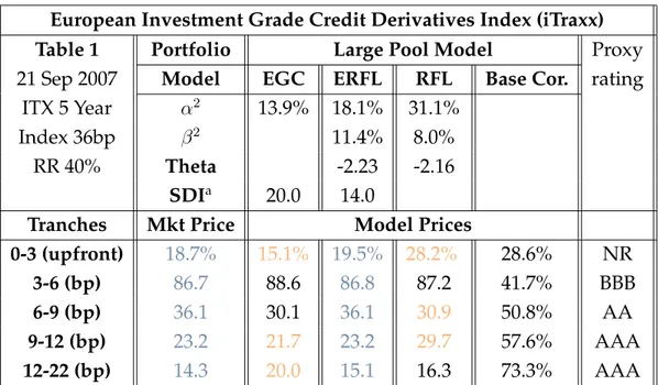
We first analyse the iTraxx case. In table 1, we display the results obtained by cali-bration of the 5 year iTraxx tranches on various versions of multi-name models, by increasing degrees of sophistication. The market data is on the September 21st, 2007 for the standard benchmarks with maturity December 20, 2012.

c

European Investment Grade Credit Derivatives Index (iTraxx)

Table 1 Portfolio Large Pool Model Proxy

21 Sep 2007 Model EGC ERFL RFL Base Cor. rating ITX 5 Year α2 _{13.9% 18.1% 31.1%}

Index 36bp β2 11.4% 8.0%

RR 40% Theta -2.23 -2.16

SDIa 20.0 14.0

Tranches Mkt Price Model Prices

0-3 (upfront) 18.7% 15.1% 19.5% 28.2% 28.6% NR

3-6 (bp) 86.7 88.6 86.8 87.2 41.7% BBB

6-9 (bp) 36.1 30.1 36.1 30.9 50.8% AA

9-12 (bp) 23.2 21.7 23.2 29.7 57.6% AAA

12-22 (bp) 14.3 20.0 15.1 16.3 73.3% AAA

European Investment Grade Credit Derivatives Index (iTraxx)

T

able

1

(continued)

Portfolio Homogeneous Model Heterogeneous Model

Model EGC ERFL RFL EGC ERFL RFL

α2 _{11% 16.6% 30.3% 10.2% 16.8% 29.8%}

β2 _{7% 3.8% 5.9% 3.2%}

θ -2.15 -2.16 -2.13 -2.13

SDI 20.8 14.0 20.8 13.0

Mkt Price Model Prices

18.7% 14.3% 19.5% 28.2% 12.7% 18.6% 26.7%

86.7 88.8 86.8 87.4 88.8 86.6 87.3

36.1 28.8 36.1 31.5 27.8 36.0 31.4

23.2 21.9 23.1 29.3 21.6 23.2 29.3

14.3 20.9 15.1 15.7 20.9 14.3 15.1

The corresponding 5 year iTraxx index level was 36bp, corresponding – under standard assumptions – to an expected loss of approximately 2.0% of the underlying portfolio. If this expected loss is realized over the 5 year horizon, the 0-3 equity tranche will be impaired by two-third of its nominal, but the 3-6 junior mezzanine (and all higher tranches) will be unimpaired. Unsurprisingly, the best calibration is obtained by the most sophisticated model (ERFL) on the most sophisticated description of the port-folio (heterogenous), with an error of 0.1bp on all tranches and less than 0.1% on the upfront price of the 0-3 equity tranche. On all the portfolio representations, the lack of

a_{SDI: systematic default intensity}

c

performance in the RFL and EGC models is significant on ”extreme” tranches, namely the junior and the senior tranches. In the RFL model, the 2 correlation regimes which are needed to adequately price the mezzanine and senior tranches are unable to cor-rectly capture the equity tranche, over-pricing its risk. It is interesting to notice the sharp contrast with the results of the EGC model. Here, in order to adequately capture the risks of the mezzanine and senior tranches, the calibration takes a “middle of the range” single correlation regime along with a relatively high SDI to force enough de-fault losses for the best names. The latter consequently overshoots the risk of the super senior 12 − 22, but the single correlation regime is “too high” and under-prices the risk of the 0-3 equity tranche.

When the heterogeneity and the term structure of the underlying single name curves is not taken into account, the consequence on a high grade portfolio is that it marginally lowers the amount of overall expected loss – a flat index level of 36 bps with no term structure implies a portfolio expected loss of 1.9% – and a more “concentrated” dis-tribution of losses around the mean: the dispersion of loss outcomes is reduced. In fact, this lower dispersion makes the “in-the-money” 0-3 equity more risky and the higher mezzanine and senior tranches comparatively less risky. Correspondingly, the ERFL calibration errors increase on the equity and the super senior tranche. The last step in the portfolio simplification is going from a homogenous but granular portfolio toward a large pool portfolio. The occurrence of a default in the granular portfolio is akin to a “default cluster” in a large pool portfolio, therefore mechanically increasing the correlation of defaults, especially for equity and mezzanine tranches. All else being equal, the large pool equity is therefore riskier; in fact, it suffers default losses, albeit infinitesimal, continuously and immediately.

European Investment Grade Credit Derivatives Index (iTraxx) Table 1 bis Portfolio Large Pool Model Proxy 06 Mar 2008 Model EGC ERFL RFL Base Cor. rating

ITX 5 Year α2 _{31.8% 27.7% 77.8%}

Index 126bp β2 11.9% 4.5%

RR 40% θ -1.2 -1.3

SDI 120.1 91.8

Tranches Mkt Price Model Prices

0-3 (upfront) 42.5% 30.5% 48.8% 59.5% 47.5% NR 3-6 (bp) 510 525.7 515.9 526.2 59.4% BBB 6-9 (bp) 321.5 304.8 319.8 264.7 66.1% AA 9-12 (bp) 231.5 212.1 232.0 232.1 71.1% AAA 12-22 (bp) 126.5 151.5 132.2 217.2 84.5% AAA c

In table 1 bis, we give large pool calibration results on the Itraxx on March 6th _2008.

While credit spread environment is very different with much wider levels, we see a similar need for the 3 levels of correlation. We observe a more frequent (θ = −1.2) and higher ”high correlation regime” (α2 _{= 27.7%). Also the systemic default intensity}

corresponds to 43% of index spread (SDI = 0.92%, RR = 40%, compared to the index at 126 bps) where it was only 23% of the index spread on September 21th _{2007 (SDI =}

0.14%, RR = 40%, compared to the index at 36 bps).

5.2

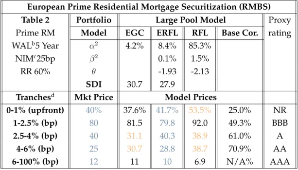
European prime RMBS and SME loan securitization

As an example of RMBS, we performed calibration on a generic European RMBS deal based on primary market statistics in the years 2004-2006 (results displayed in table 2)

European Prime Residential Mortgage Securitization (RMBS)

Table 2 Portfolio Large Pool Model Proxy

Prime RM Model EGC ERFL RFL Base Cor. rating WALb_{5 Year α}2 _{4.2% 8.4% 85.3%}

NIMc_{25bp β}2 _{0.1% 1.5%}

RR 60% θ -1.93 -2.13

SDI 30.7 27.9

Tranchesd Mkt Price Model Prices

0-1% (upfront) 40% 37.6% 41.7% 53.5% 25.0% NR

1-2.5% (bp) 80 81.5 79.8 92.0 49.3% BBB

2.5-4% (bp) 40 31.1 40.3 38.9 61.0% A

4-6% (bp) 25 30.7 28.8 38.7 70.9% AA

6-100% (bp) 12 11 10 6.9 N/A% AAA

The EGC and RFL models have poor calibration and discrimination of A and AA tranches, whereas the ERFL model appears to be sufficient within the large pool ap-proximation. The conclusion we draw is the necessity of the 3 correlation regimes. In comparison to the Itraxx calibration, we observe an ”almost independent” regime of correlation (which corresponds to β2 _{= 0, 1%), a lower correlation (β}2 _{= 8, 4%) in the}

stress regime and higher influence of the systemic risk, corresponding to 45% of the pool’s spread (SDI = 0.28% , RR = 60%, compared to a pool NIM of 25 bps).

b_{Weighted Average Life} c_{Neat Interest Margin}

d_{Attachment points include benefit of 0.4% reserve account from excess spread}

c

We also performed the calibration of a generic European SME loan deal based on pri-mary market statistics in the years 2000-2006 (results displayed in table 3).

European SME loans securitization

Table 3 Portfolio Large Pool Model Proxy

SME Model EGC ERFL RFL Base Cor. rating

WAL 4 Year α2 _{7.1% 8.0% 59.0%}

NIM 75bp β2 0.1% 5.0%

RR 50% θ -1.8 -2.06

SDI 46.1 38.2

Tranchese _{Mkt Price Model Prices}

0-4% (upfront) 35% 32.2% 35.2% 40.2% 23.5% NR 4-6% (bp) 120 122.1 120.8 120.4 34.1% BBB

6-8% (bp) 65 57.4 65.1 54.8 42.5% A

8-11% (bp) 40 47.4 41.9 53.0 52.4% AA

11-100% (bp) 18 20.1 16.7 10.7 N/A AAA

The correlation regimes are closed to the RMBS calibration, and we again observe the necessity of 3 correlation regimes. But the systemic risk influence is much more similar to the IG index (25% of the composite spread, SDI = 0.38%, RR = 50%, compared to pool NIM of 75 bps).

The main conclusion of the calibration on those three different products is that ERFL model parameters interpretation is valuable in a broader universe of ABS and multi-name credit assets. Based on pre-crisis market levels calibrations, ERFL parameters are more informative than base correlation:

• They suggest serious shortcomings of classical correlation neutral strategies. • Super senior risks captured by composite spread instead of correlations. Across credit asset classes, we observe

• Corporate credit risk has a higher correlation than SME or Retail credit in normal and stress regime (as could be expected).

• Residential mortgage credit has a higher proportion of systemic risk in the com-posite spread, which can be explained by several factors: importance of the real estate markets, leverage of households, banks concentration in the segment, jobs and real economy.

e_{Attachment points include benefit of 1.4% reserve account from excess spread}

c

6

Conclusion

Our results show that a simplistic composite closed-form model using a large pool ap-proximation together with a systematic default risk parameter can achieve calibration results that can nevertheless frequently outperform the calibration results obtained by a sophisticated random factor loading (RFL) model, with the full description of the portfolio underlying single names curves, but which lacks this SDI or “crash risk” pa-rameter. In our backtesting, the calibrated parameters on iTraxx and CDX since 2006 turn out to be very stable with respect to the market datas. This model provides an an-swer to some of the shortcomings of copula based models, and gives parameters which enjoy a real economic interpretation. These results are achieved with the introduction of this SDI parameter and the current ”sub-prime” crisis provides clear elements in its favour. Fear contagion, liquidity squeeze, loss of confidence in origination standards or rating methodologies happen with 100% correlation(!). This recent liquidity crisis, triggered by the contagion to all credit markets by the fear of US sub prime losses illus-trates even more the magnitude and correlation of this risk premium that can affect all credit assets, almost irrespective of credit quality or ratings. Taking into account these phenomena through a systematic default parameter is obviously a simplification, but it goes a long way in the right direction to explain both the long term risk premium as well as the occasional spikes seen in situations of crisis. We could even further argue that structured credit disasters such as CDOs of mezzanine HEL ABS could have been avoided through the use of this model. It would have required a much higher AAA CDO of ABS credit enhancement from the high proportion of SDI in the composite spread. As a consequence, more scrutiny would have resulted on BBB pieces of HEL ABS, which could no longer be channelled to CDO of ABS.

In our view, this approach demonstrates that simple core ingredients of credit mod-elling can still be fruitfully applied to address the pricing of credit derivatives and structured credit productsf_.

References

[AS2005] L. Andersen and J. Sidenius, Extensions to the Gaussian Copula: Random Recovery and Random Factor Loadings, Journal of Credit Risk, 2005.

[BR2002] T. Bielecki and M. Rutkowski, Credit Risk: Modeling, Valuation and Hedging, Springer-Verlag, Berlin, 2002.

[Sch2003] Ph. Sch ¨onbucher, Credit Derivatives Pricing Models, Wiley, 2003.

f_{Complementary insights can be found in [LPV2009]}

c

[LB2005] M. Trinh, R. Thompson and M. Devarajan, Relative Value in CDO Tranches: A View through ASTERION QCR Quarterly, Q1 2005.

[LPV2009] Jean-Pierre Lardy, Fr´ed´eric Patras and Franc¸ois-Xavier Vialard. Correlation, CDOs of ABS and the subprime crisis, in: Financial Risks: New Developments in Structured Product and Credit Derivatives. Eds: Christian Gourieroux and Monique Jeanblanc, Economica (to appear, 2009).

c