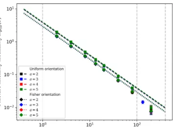
On the Density Variability of Poissonian Discrete Fracture Networks, with application to power-law fracture size distributions
Texte intégral
Figure

Documents relatifs
It has to be emphasized that the presence of the accelerometer on-board not only enables fundamental physics objectives to be met, but also constitutes an invaluable complement to
Au lieu de trois valeurs RVB, nous disposons donc en chaque pixel (u, v) d’un seul niveau de couleur dans un canal corres- pondant à la matrice de Bayer (cf. L’intensité d’un
Le but de cette thèse est de lever ces différentes limitations notamment en mettant au point une technique de fabrication stabilisée de substrats germes GaAs
We proved directly by dynamic light scattering (DLS) and cryogenic electron microscopy (cryo-TEM) that the substrate is encapsulated in the micelles after deprotonation,
CRITICAL: Removal of all culture medium from the ring and the forceps is essential, as the addition of culture medium near the aortic ring significantly decreases the local
Dans cet article, nous avons introduit IJTI, un nouvel algorithme d’inférence incré- mentale par JT qui est conçu pour les systèmes multi-cibles dynamiques. En supposant
/ La version de cette publication peut être l’une des suivantes : la version prépublication de l’auteur, la version acceptée du manuscrit ou la version de l’éditeur. For
Dans cet article, nous ne cherchons pas à calculer l’effet sur l’emploi d’un scénario ou d’une politique de transition énergétique mais à estimer le contenu en emploi et en
