HAL Id: hal-00437515
https://hal.archives-ouvertes.fr/hal-00437515
Submitted on 1 Jan 2016
HAL is a multi-disciplinary open access
archive for the deposit and dissemination of
sci-entific research documents, whether they are
pub-lished or not. The documents may come from
teaching and research institutions in France or
abroad, or from public or private research centers.
L’archive ouverte pluridisciplinaire HAL, est
destinée au dépôt et à la diffusion de documents
scientifiques de niveau recherche, publiés ou non,
émanant des établissements d’enseignement et de
recherche français ou étrangers, des laboratoires
publics ou privés.
GOMOS/ENVISAT stellar occultation instrument
Kristell Pérot, Alain Hauchecorne, Franck Montmessin, Jean-Loup Bertaux,
Laurent Blanot, Francis Dalaudier, Didier Fussen, Erkki Kyrölä
To cite this version:
Kristell Pérot, Alain Hauchecorne, Franck Montmessin, Jean-Loup Bertaux, Laurent Blanot, et al..
First climatology of polar mesospheric clouds from GOMOS/ENVISAT stellar occultation
instru-ment. Atmospheric Chemistry and Physics, European Geosciences Union, 2010, 10 (6), pp.2723-2735.
�10.5194/acp-10-2723-2010�. �hal-00437515�
www.atmos-chem-phys.net/10/2723/2010/ © Author(s) 2010. This work is distributed under the Creative Commons Attribution 3.0 License.
Chemistry
and Physics
First climatology of polar mesospheric clouds from
GOMOS/ENVISAT stellar occultation instrument
K. P´erot1, A. Hauchecorne1, F. Montmessin1, J.-L. Bertaux1, L. Blanot2, F. Dalaudier1, D. Fussen3, and E. Kyr¨ol¨a4
1LATMOS-IPSL, CNRS/INSU, UMR 8190, UPMC Univ. Paris 06, Univ. Versailles St-Quentin, Guyancourt, France
2ACRI-st, Sophia Antipolis, France
3BIRA-IASB, Brussels, Belgium
4FMI, Helsinki, Finland
Received: 26 October 2009 – Published in Atmos. Chem. Phys. Discuss.: 30 November 2009 Revised: 9 March 2010 – Accepted: 12 March 2010 – Published: 23 March 2010
Abstract. GOMOS (Global Ozone Monitoring by
Occul-tation of Stars), on board the European platform ENVISAT launched in 2002, is a stellar occultation instrument com-bining four spectrometers and two fast photometers which measure light at 1 kHz sampling rate in the two visible chan-nels 470–520 nm and 650–700 nm. On the day side, GO-MOS does not measure only the light from the star, but also the solar light scattered by the atmospheric molecules. In the summer polar days, Polar Mesospheric Clouds (PMC) are clearly detected using the photometers signals, as the solar light scattered by the cloud particles in the instrument field of view. The sun-synchronous orbit of ENVISAT allows ob-serving PMC in both hemispheres and the stellar occultation technique ensures a very good geometrical registration. Four years of data, from 2002 to 2006, are analyzed up to now. GOMOS data set consists of approximately 10 000 cloud ob-servations all over the eight PMC seasons studied. The first climatology obtained by the analysis of this data set is pre-sented, focusing on the seasonal and latitudinal coverage, represented by global maps. GOMOS photometers allow a very sensitive PMC detection, showing a frequency of oc-currence of 100% in polar regions during the middle of the PMC season. According to this work mesospheric clouds seem to be more frequent in the Northern Hemisphere than in the Southern Hemisphere. The PMC altitude distribution was also calculated. The obtained median values are 82.7 km in the North and 83.2 km in the South.
Correspondence to: K. P´erot
1 Introduction
Noctilucent clouds (NLC), also termed Polar Mesospheric Clouds (PMC) when observed from satellites, are Earth’s highest clouds, located in the atmospheric region just below the polar summer mesopause at an altitude of about 83 km. They typically occur at latitudes greater than 55◦ in both hemispheres during a period of approximately three months around the summer solstice. These clouds are composed pri-marily of water ice particles (Hervig et al., 2001; Eremenko et al., 2005). In the atmospheric region where they form, the pressure is about one hundred thousand times less at the surface and the air may be as much as a million times drier than the surface desert air (Sonnemann and Grygalashvyly, 2005), so extremely low temperatures are essential to allow the PMC formation. Such conditions only occur at the sum-mertime polar mesopause, which is the coldest place on earth with minimum temperatures below 140 K (L¨ubken, 1999). These extraordinary low temperatures can be explained by strong vertical motions, driven by the breaking of vertically propagating gravity waves. In the summer polar mesosphere, a strong upward motion is associated with adiabatic cool-ing of air. When seen by ground-based observers, NLC or “night-shining” clouds, resemble normal cirrus clouds ex-cept they can only be seen when the sun is below the horizon (Fig. 1). Indeed, at evening or morning twilight, the lower atmosphere is already in the dark, but the upper mesosphere is still sunlit.
First identified 120 years ago (Leslie, 1885), many issues about PMCs remain unresolved: “In short, we do not
un-derstand what causes a mesospheric cloud to form or how it evolves” (Russell et al., 2009). The answer to these
24
Fig. 1. Noctilucent cloud photographed by Kristell Pérot during the LPMR-09 meeting, 14
July 2009, Djurö island, Stockholm archipelago, Sweden
Fig. 1. Noctilucent cloud photographed by Kristell P´erot during
the LPMR-09 meeting, 14 July 2009, Djur¨o island, Stockholm archipelago, Sweden.
observations go back to 1885. Although the clouds are ob-served since a long period, the information gathered per year has significantly increased in recent decades due to the use of many new instruments. Their morphology and evolution have been studied using sounding rockets (e.g. Walchli et al., 1993; Gumbel and Witt, 1998; Goldberg et al., 2006) and lidars (Hansen et al., 1989; Thayer et al., 2003; Chu et al., 2006; Fiedler et al., 2009). Observed from satellite for the first time in the early 1970s (Donahue et al., 1972), since then noctilucent clouds have been monitored more or less continuously since the late 1970s by a variety of satellite-based instruments employing different measurement tech-niques (see Deland et al., 2006, for an overview of the ex-isting satellite data sets). The Aeronomy of Ice in the Meso-sphere (AIM) mission, launched in 2007 by NASA, is the first satellite mission entirely dedicated to the study of polar mesospheric clouds (Russell et al., 2009). All these measure-ments have yielded a great deal of information on PMC prop-erties, including the altitude and geometric extent of clouds, the size and composition of cloud particles, seasonal and multidecadal trends in cloud frequency and brightness, and their dependence on solar activity. Related parameters which have a significant influence on PMC formation (e.g. temper-ature, water vapor, turbulence, meteoric dust and ionization) are also measured.
These clouds which form at the “edge of space” have re-cently focused more and more attention, not only because of their formation process, but also for the information they re-veal about the mesospheric environment. They are indeed very sensitive to changes in that environment. They occur more frequently, appear brighter and seem to form at lower latitudes than ever before (Taylor et al., 2002; Deland et al., 2007). Deland et al. (2003, 2007) have found a long-term increase in the PMC frequency and brightness over the 27 years of observations from the solar backscattered ultraviolet
(SBUV) series of instruments. This behavior is not under-stood yet, and it suggests they could be considered as a pos-sible indicator of long-term global change in the mesosphere (Thomas and Olivero, 2001). Indeed they may be a phe-nomenon associated with the rise of greenhouse gases in the atmosphere (Thomas et al., 1989, 1991) and they are there-fore expected to respond to long-term climate change. But the discussion about this issue is controversial up to now (von Zahn, 2003; Thomas et al., 2003). A detailed analysis on the main PMC properties observations is still outstand-ing. It is important to study the mean and variations of cloud layer properties to generate a robust basis for interpretation of potential changes in the atmosphere, but it is equally im-portant to gather information on the microphysical processes involved in the cloud particles formation (see recent results of Murray et al., 2009; Zasetsky et al., 2009a; and Zaset-sky et al., 2009b, about the nucleation mechanism and for-mation rates). Mesospheric clouds variations are observed to occur on different scales, from small scales connected to gravity waves and turbulence (Gerrard et al., 2004) to the largest (Deland et al.,2003, have seen an anticorrelation be-tween PMC occurrence frequency and 11-years cycle of so-lar activity from SBUV data set), through the medium scales connected to tidal variations or planetary waves for example (Fiedler et al., 2005; Merkel et al., 2003).
The present work comes at a time of great interest and rapid improvement in our understanding of polar meso-spheric clouds. Around the globe, researchers make com-prehensive observations of these clouds with ever higher ca-pabilities instruments. Observations can be ground-, rocket-or space-based. This progress is accompanied by advances in modelling capabilities (Berger and L¨ubken, 2006; Merkel et al., 2009). International working group on Layered Phenom-ena in the Mesopause Region (LPMR) aims to develop and facilitate collaborations among different communities and different countries. In this paper, the first climatology of po-lar mesospheric clouds obtained from the GOMOS (Global Ozone Monitoring by Occultation of Stars) data analysis is presented. It is organized as follows. Section 2 summarizes the basic instrument design, sampling characteristics of the instrument and the measurement technique. Section 3 then describes the PMC detection algorithm used to generate the GOMOS PMC data set. The first results are finally presented in Sect. 4, including an analysis of the cloud detection fre-quency, seasonal and latitudinal distribution of PMC obser-vations, and also a first estimation of the cloud altitude dis-tribution, followed by a summary and conclusions.
2 GOMOS stellar occultation instrument
GOMOS is one of the three instruments with MIPAS (Michelson Interferometer for Passive Atmospheric Sound-ing) and SCIAMACHY (SCanning Imaging Absorption spectroMeter for Atmospheric CHartographY) flying aboard
25
Fig. 2. Principle and geometry of the GOMOS stellar occultation measurements. In the top
right: example of an intensity profile measured by the photometers during an occultation event on the day side.
Fig. 2. Principle and geometry of the GOMOS stellar occultation measurements. In the top right: example of an intensity profile measured
by the photometers during an occultation event on the day side.
the European Space Agency’s ENVISAT platform to study the atmosphere of the Earth. This satellite was launched with Ariane 5 on 1 March 2002 in Kourou (Guyana). It operates in a 800 km sunsynchronous orbit with a period of 100.6 min. GOMOS had its first occultation on 20 March. Since then, it is operating smoothly and has collected almost 700 000 oc-cultations. It has already provided up to seven years of data to analyze. This instrument was designed to monitor ozone and other related species from the upper troposphere to the lower thermosphere (about 15 to 100 km) with a very high accuracy using the technique of stellar occultation. It is the first space instrument dedicated to the study of the Earth by this technique (see Bertaux et al., 2004, and Kyr¨ol¨a et al., 2004, for more details).
It is constituted by four spectrometers and two fast pho-tometers. The spectrometers work in the ultraviolet-visible wavelengths 250–675 nm and two additional channels are lo-cated in the near-infrared centered at 760 and 940 nm. But this PMC analysis is performed exclusively with the pho-tometers, at least for the moment. They measure light at 1 kHz sampling rate, one of them in the blue wavelength re-gion and the other in the red. Their signals are integrated over the wavelength range 470–520 nm and 650–700 nm, respec-tively. They are initially aimed to correct star scintillation perturbations and to determine high vertical resolution tem-perature profiles. But, in the summer polar days, they also clearly detect the solar light scattered by the PMC particles.
The principle of stellar occultation is illustrated in Fig. 2. GOMOS is implemented on ENVISAT opposite to the ve-locity vector and looks at various stars while the platform is
moving along its orbit. When a star sets behind the atmo-sphere, its light crosses quasi-horizontally the atmosphere in a limb geometry and travels a long distance in layers just above the tangent point defined as the location of lowest al-titude. The telescope captures the star at a tangent height around 150 km, locks to it and follows it down to about 10 km. This technique allows a nearly perfect knowledge of the tangent altitude, only depending on the geometry of the light path between the star and the satellite. The photome-ters altitude registration is better than 100 m and the vertical resolution defined by the field of view is lower than 1 km. In Fig. 2 is represented an example of intensity profile mea-sured by the photometers during an occultation event on the day side. Tangent altitude is plotted as a function of mea-sured intensity. The signal corresponds to the light of the star, but also to scattered solar light. It will be described in more details in the next section.
Besides the self-calibration and the very good vertical res-olution, the advantage of the stellar occultation method is a very good geographical and temporal coverage ensured by the multitude of suitable targets (180 different stars can be aimed by GOMOS). Up to about 450 occultations are ob-served each day at almost all latitudes. Moreover measure-ments are obtained from both night and day side of the Earth but, as it will be explained in the Sect. 3.2, only day side cases are taken into account in this study. Consequently, the win-ter pole, immersed in the polar night, is not analyzed here. This, however, does not affect our results on PMC climatol-ogy as these clouds do not form in the winter mesosphere. Nevertheless GOMOS measurements distribution presents a
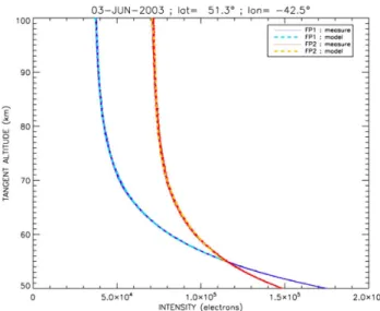
26 Fig. 3. Signals measured by GOMOS photometers (FP1: [470 ; 520] nm and FP2: [650 ; 700] nm) during an occultation event on the day side. At high altitude, the recorded signal mostly corresponds to star light. It is increasing downward due to the contribution of atmospheric Rayleigh scattering of the bright limb.
Fig. 3. Signals measured by GOMOS photometers (FP1: 470;
520 nm and FP2: 650; 700 nm) during an occultation event on the day side. At high altitude, the recorded signal mostly corresponds to star light. It is increasing downward due to the contribution of atmospheric Rayleigh scattering of the bright limb.
bias that must be noted. It is indeed characterized by a size-able asymmetry between North and South. The observations performed around the North Pole can be numerous and very close to the pole, but the South Pole is less well observed. GOMOS provides no measurement at latitude higher than 80◦S. This can be explained by the ENVISAT orbital prop-erties, as well as the GOMOS observation geometry. Indeed, the satellite’s orbit is quasi-polar, so it does not get exactly over the pole. It gets actually slightly over the right of the North Pole and over the left of the South Pole. As previ-ously explained, the GOMOS field of view is headed back-wards: the instrument observes in the opposite direction to the moving speed of the satellite on its orbit. The azimuth of the pointing direction with respect to the orbital plane ranges between −10◦ and 90◦, which explains why the re-gion surrounding the South Pole is still invisible for this in-strument. Moreover the local time of the descending node is 10:00. This means that, when ENVISAT is flying above the South Pole, the angle between the Sun and the line of sight is lower than above the North Pole. Angles smaller than 40◦are forbidden in order to protect the detector against sunlight. The stars which can be observed are therefore less numerous. Moreover, the number of observations and their latitudinal distribution are different for the two hemispheres, even at latitudes lower than 80◦. During the PMC season, at latitudes higher than 55◦(and lower than 80◦), where the clouds are most likely to occur, the observations are 6% more numerous in the South than in the North up to 70◦, but they are 50% less numerous between 70◦and 80◦. The difference in local time should also be noted (for most observations, at midmorning for the North and in the early morning for the South), because the PMC occurrence frequency is strongly
influenced by local time (e.g. Fiedler et al., 2005; Stevens et al., 2009; Shettle et al., 2009). As we shall see later, for all these reasons, the results obtained for the two hemispheres cannot always be directly compared because of this asym-metry. This must be taken into account in the analysis.
3 PMC detection algorithm 3.1 Photometers data description
When GOMOS points to a star, tangential (defined between the line of sight and a hypothetical sphere centered on the Earth center) altitude is about 150 km initially. At such al-titude, the light can be considered as being fully transmitted by the atmosphere without any loss caused by absorption or scattering. As previously explained, the instrument pointing is locked to the star throughout the sequence. As the satel-lite is moving along its orbit, the beam of light goes through thicker layers of the atmosphere until the star is completely occulted at low altitude. For each occultation sequence, each photometer records a vertical profile of intensity, propor-tional to the luminous flux impacting the pixels, as shown in Fig. 3, an example with no PMC. The measured signal does not correspond only to the light of the star, but also con-tains contributions from other sources. The sensor indeed detects the solar light scattered at the limb by the molecules (Rayleigh scattering) or by particles. The intensity of the light scattered according to Rayleigh theory is proportional to the atmospheric density integrated along the line-of-sight, so it decreases exponentially with the altitude. This explains the exponential shape of the curve.
As one can notice on Fig. 3, intensity is always greater in the blue channel than in the red one below roughly 55 km. In the lower mesosphere, Rayleigh scattering dominates, so the light is more scattered at shorter wavelengths. At higher altitude, the recorded signal is essentially that of the star.
3.2 Effect of a PMC on photometers signals
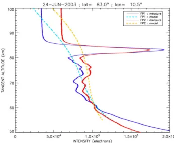
In Fig. 4 are plotted photometers signals in the case where a PMC is present. The light is scattered by the cloud particles. The scattering process can be represented by the Mie The-ory, which is, in this case, very close to Rayleigh scattering. The cloud particles are indeed much smaller than the wave-length of the incident light, with a radius of about 50 nm, according to various measurements (e.g. Rusch et al., 1991; Von Savigny et al., 2005; Baumgarten et al., 2007; Lumpe et al., 2008). In an optically thin regime, scattered intensity is proportional to tangential opacity, i.e. the number of scatter-ing particles encountered along the line-of-sight weighted by their effective cross section. The presence of a cloud is read-ily distinguishable as it creates a prominent peak in the verti-cal profile. Most profiles also present several other peaks be-low the main one. These secondary peaks are due to the part of the cloud which is not located at the tangent point during
measurement. This explains why they are associated with a lower tangent altitude. Small (with respect to the incident wavelength) cloud particles explain why the blue photome-ter is always more sensitive to the presence of a PMC than the red one. In its most general form, the measured signal
Smeas(z), where z denotes the tangent altitude, is given by the following sum of 4 components:
Smeas(z) = Sstar(z) + Smol(z) + SPMC(z) + Sstraylight
where Sstar(z) is the stellar contribution, Smol(z) and SPMC (z) are the components associated with the scattering of the solar light, respectively by the atmospheric molecules and by the PMC particles. The term Sstar (z) can be assumed to be constant at first order, independent of altitude. Smol (z) is present at all altitudes as an exponentially varying back-ground, and dominates at altitudes below the cloud, where
the atmosphere is denser. The atmospheric extinction is
negligible above 50 km of altitude in the considered wave-lengths. Photometers also detect a stray light component
Sstraylight. Any light which is not emitted by a source located in the GOMOS field of view is considered as stray light. The origin of this light is not very well established yet. It could be partly due to the scattering of solar light by thick and large tropospheric cloud systems and further scattering from the tracking mirror of GOMOS.
Figure 4 is only an example of the effect that a PMC can have on the signal. Some clouds generate a much smaller, hardly detectable distortion. Others deform the measured profile in a more complex way, which leads to the emergence of more numerous peaks in a wider range of altitudes. Even if the PMC contribution has a finite extent in the measured profile, it can be smeared out somewhat by the horizontal extent of the cloud along the line-of-sight.
Only day side cases are considered in this study, since mesospheric cloud detection relies on solar light scattered by the particles, which in the case of the solar beam is propor-tional to the field of view of the photometers and thus makes it more sensitive than observation at night, where detection would only rely on a slight, barely perceptible dimming of the star light by the cloud. More precisely, only cases with a solar zenith angle (SZA) lower than 94◦were studied, be-cause, at wider angles, the mesospheric clouds are not sun-lit enough to be detected (the SZA considered here is not measured at ground level, but corresponds to the SZA at the tangent point, averaged for each occultation between 50 and 100 km).
These day light measurements are very efficient at detect-ing noctilucent clouds, usdetect-ing the algorithm described below.
3.3 Detection algorithm description
The goal of the detection algorithm is to isolate any profile where a PMC signature SPMCis present. The most accurate way to do that is to model the shape the profiles would take if
27 Fig. 4. Example of GOMOS photometers (FP1: [470 ; 520] nm and FP2: [650 ; 700] nm) signals on which we can observe a PMC feature
Fig. 4. Example of GOMOS photometers (FP1: 470; 520 nm and
FP2: 650; 700 nm) signals on which we can observe a PMC feature.
there were no clouds along the line-of-sight. The methodol-ogy which yields the most accurate estimate is a least square fitting routine, which finds a polynomial fit of degree 3 of the signal between 55 and 100 km. This fit is carried out on each profile. Each fitted curve, represented by a dashed line on Figs. 3 and 4, is then compared to its correspond-ing original profile (i.e. the one that it was fitted to). If a PMC is present (Fig. 4), the two curves will be different to a detectable amount. The quantitative detection criterion is based on a chi square calculation between this modelled pro-file and the measured one. As shown on Fig. 3, when there is no PMC, the light curves are perfectly fitted and the χ2 is small. However we can see on Fig. 4 that the two curves are significantly different for each photometer. A noctilu-cent cloud event will therefore be characterized by a high chi-square value. The standard deviation σ of the measured intensity, used in the χ2 determination, is calculated using a 100-point running boxcar average around the point of in-terest. This smoothing significantly improves the reliability of the results. Given the χ2 values calculated for each oc-cultation and for each of the two photometers we can then define detection criteria for these clouds. Both photometers are used to minimize the risk of error. We define a PMC to be present if the measured intensity profile meets the following two criteria:
1. The obtained chi-square value is greater than a threshold value of 1.8 in the two channels.
2. The chi-square value associated with the blue photome-ter is greaphotome-ter than the value associated with the red one.
The choice of the 1.8 threshold is based upon a sensitivity analysis in which the detection algorithm was run on a large sample of data, using various thresholds. For each of them,
the results were compared to the measured profiles to verify if detected PMC corresponded to a real cloud. The value of 1.8 is the one which gave the best results, i.e. which gave the same number of detections as a human eye would.
For all GOMOS measurements, intensity profiles are con-sidered for the two photometers. This methodology was ap-plied to all available measurements from late August 2002 to early July 2006. Almost 200 000 events were thus pro-cessed over these four years, but some errors (false detec-tions) remain. Some mesospheric clouds were indeed de-tected although they were not expected. The verification of these cases confirmed these were false positive detections. These errors were due to spurious stray light contamination. As previously told, the origin of this light is not very well un-derstood yet. In most cases this component can be assumed constant, so it is not a problem to model the profile with-out the cloud contribution. But in some much more com-plex cases, the profiles are characterized by very strong vari-ations of the intensity as a function of altitude, which is how a mesospheric cloud is generally detected. In these cases how-ever, they correspond to measurements made at middle lati-tude. This component could have several causes, but it seems principally due to the reflection of solar light by tropospheric cloud systems. Sometimes the instrument observes above a region where there are large convective systems in the tro-posphere. Cumuli are very high and very reflecting clouds, so they can redirect light into GOMOS field of view through scattering on the tracking mirror. Some of these profiles were compared to photographs taken by METEOSAT at the same time and at the same place. The cloud cover was indeed very important, and the irregular spatial structure of these clouds appeared to explain the observed variations of light intensity. The second detection criterion noted above aims at limiting this problem. In most of these cases the chi-square value calculated for the red photometer is indeed greater than the one associated with the blue photometer, which is not possi-ble in the case of a PMC feature, as explained before. But unfortunately, this condition does not suffice to eliminate all errors due to the stray light. Because of this problem, the de-veloped methodology is not fully automatic. Errors of this kind are rare (they correspond to only 1.7% of the detec-tions). However it is necessary to eliminate them in order to ensure the accuracy of results. This problem is never met at high latitudes, so the results obtained in the summer polar region are correct. All cases where such errors are likely to appear (i.e. all clouds detected at another time than June–July above 65◦N or December–January below 65◦S) must be ver-ified, which can be made rather quickly with the sole hu-man eye. Indeed they cannot be confused with mesospheric clouds which create a characteristic distortion. A correction of the result is applied if necessary. It ensures that each de-tection corresponds to a real mesospheric cloud.
However some of the dimmest clouds are inevitably missed. Very thin clouds, whose effect on the photometers signals is barely visible, cannot be detected. But these cases
are rare, because the threshold value of 1.8 was chosen to ensure the highest possible accuracy. Indeed, the algorithm was set to detect thin clouds, even if it involves more numer-ous false positive detections, and therefore a longer time of verification.
This work eventually led to an accurate detection algo-rithm to detect noctilucent clouds, which will be subse-quently used to conduct a comprehensive study of these clouds at the edge of space.
4 First results
4.1 Global PMC maps
As previously told, the detection algorithm described in Sect. 3 was run on four years of GOMOS data, which range from late August 2002 to early July 2006, to yield an ini-tial set of potenini-tial PMC events. Almost 10 000 noctilucent clouds were detected thanks to this method.
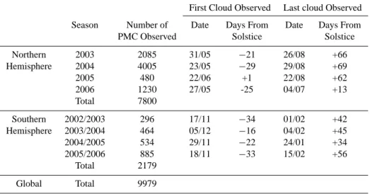
These results are summarized in Table 1, which lists the number of clouds observed during each period, and the dates when the first and last clouds occurred (“deadlines” in the following). This table helps to highlight the important differ-ence in the observation distribution between the two hemi-spheres. Indeed, 78% of PMC were detected in the north. As explained in Sect. 2, the South Pole is far less observed than the North Pole. This obviously affects significantly the number of clouds which can be observed. The deadlines also depend on the distribution of observations, which can be well visualized on Fig. 8, described in the following. For exam-ple, it appears that the NH season 2005 started unusually late (on day+1 relative to summer solstice). This late start is con-nected to lack of data, due to technical problems of the in-strument, rather than a delayed onset of the PMC season.
Our detection algorithm yielded a very rich PMC data set which can be graphically summarized by global maps. Fig-ure 5 shows the example of one year of data between 2003 and 2004. Each panel shows a map centered on the pole. The red symbols denote the location of all GOMOS mea-surements made during the given period, and the blue ones represent all events where a PMC was detected. The left col-umn corresponds to a PMC season in the Southern Hemi-sphere, and the right one to the PMC season in the Northern Hemisphere, the same year. In both cases these maps allow to visualize the evolution of clouds during the summer, from their appearance around the pole to their disappearance. For more details such maps were drawn every two weeks, for the four years considered and for the two hemispheres. For each of them the corresponding PMC detection frequency is also indicated. This quantity is the most useful measure of PMC occurrence in the GOMOS data set. This value strongly depends on observations distribution. Differences in sam-pling frequency from one period to another are apparent from variations in spatial density of red dots on each map. The
Table 1. Number of PMC detected by GOMOS and timing of first and last clouds in each season and for each hemisphere. The deadlines
also depend on the observations distribution (e.g. the late start of the NH season 2005 is connected to lack of data, due to an instrumental problem, rather than a delayed onset of the PMC season.).
First Cloud Observed Last cloud Observed Season Number of Date Days From Date Days From PMC Observed Solstice Solstice Northern 2003 2085 31/05 −21 26/08 +66 Hemisphere 2004 4005 23/05 −29 29/08 +69 2005 480 22/06 +1 22/08 +62 2006 1230 27/05 -25 04/07 +13 Total 7800 Southern 2002/2003 296 17/11 −34 01/02 +42 Hemisphere 2003/2004 464 05/12 −16 04/02 +45 2004/2005 534 29/11 −22 24/01 +34 2005/2006 885 18/11 −33 15/02 +56 Total 2179 Global Total 9979
observations distribution depends on the ENVISAT orbital properties, on the GOMOS observation geometry and on the aimed stars. There are always more measurements at high latitude, which corresponds very well to what we need to study the polar mesospheric clouds. The geographical cover-age is very good, but we can also see on Fig. 5 that, as told in Sect. 2, the measurements are closer to the pole in the North-ern Hemisphere than in the southNorth-ern one. This explains why the PMC detection frequencies are much higher in the North than in the South.
These maps allow a very good display of the results, but are not sufficient for an accurate interpretation.
4.2 PMC detection frequency
The PMC frequency of occurrence was then calculated in two weeks time bins, rather than every month. This quantity is simply obtained by dividing the number of PMC detected in the two weeks considered by the total number of corre-sponding GOMOS measurements. Figure 6 was obtained by plotting these values in the form of a histogram, for the two hemispheres. This provides a good picture of the evolu-tion of PMC throughout each season and its variability from year to year. Clouds appear over a period of approximately three months during the local summer. Their evolution is very fast: they appear in a few days and disappear as quickly. These results show a great amount of interannual variability in the observed frequencies. The origin of these variations is not yet understood, but they can in part be explained by the interhemispheric stratosphere-mesosphere coupling that can affect PMC population (Karlsson et al., 2007). This year-to-year variability is also observed in other studies. For exam-ple, L¨ubken et al. (2009) also found a significant decrease
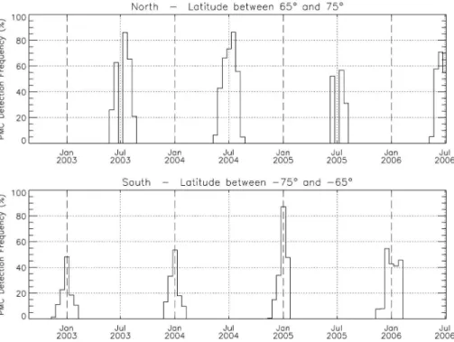
in the occurrence frequency in 2005 in the Northern Hemi-sphere with the LIMA model (Leibniz-Institute Middle At-mosphere model). This figure also shows some interhemi-spheric differences. For the most part, frequencies in the core of the PMC season vary between 5% and 85% within a sea-son in the North, and between 10% and 50% in the South (with an exception in January 2005 in the Southern Hemi-sphere, where GOMOS saw clouds in approximately 85% of its measurements). Therefore noctilucent clouds seem to be more frequent in the north than in the south, but it needs to be discussed. We must keep in mind that frequency values are strongly dependent on observations distribution. It is dif-ficult to distinguish what is due to an irregular distribution or what is a real trend, even if, in each hemisphere, only the lat-itudes between 65 and 75 degrees are considered, where the observations distribution is better. In general, clouds occur most frequently in mid-July in the North and in early January in the South. During certain seasons the values fall to zero. This is caused by significant data loss due to instrumental problems, particularly in 2003 and 2005, which might affect the PMC statistics. Indeed the fact that no PMC were ob-served in these periods is simply a consequence of sampling biases. Fortunately, these unavailability periods do not, if not slightly, overlap the time bins in which were calculated the frequency values shown in Fig. 6. Therefore the reliability of these values was not affected by the technical problems encountered, and this figure gives a good overview of first results.
Figure 7 allows a more accurate study of the evolution of the PMC detection frequency during a season. In this ver-sion, the frequency was also calculated in 2-weeks time-bins in the same latitude band, but this time combining the four years of data. When year to year variations are averaged out
Fig. 5. Example of maps for the two PMC seasons in 2003/2004, in the Southern Hemisphere
on the left, and in the Northern Hemisphere on the right. Each map corresponds to one month.
The red symbols represent all GOMOS measurements made during the considered month,
while the blue symbols indicate the location of all events where a PMC was detected. For
each map, the PMC detection frequency is also indicated.
Fig. 5. Example of maps for the two PMC seasons in 2003/2004,
in the Southern Hemisphere on the left, and in the Northern Hemi-sphere on the right. Each map corresponds to one month. The red symbols represent all GOMOS measurements made during the con-sidered month, while the blue symbols indicate the location of all events where a PMC was detected. For each map, the PMC detec-tion frequency is also indicated.
what remains is a smooth, symmetric seasonal distribution, of a roughly three months period. It is obvious from this fig-ure that the GOMOS PMC observations are peaked about 20 days after the summer solstice for both hemispheres, which is consistent with other studies on this subject (e.g. Thomas et al., 1991; Petelina et al., 2006; Lumpe et al., 2008; Fiedler et al., 2009; Robert et al., 2009). The obtained values range from approximately 10 to 80 % during the period from about 30 days before solstice to 70 days after in the North, and from 5 to 55 % from about 35 days before solstice to 55 days after in the South. So noctilucent clouds seem to be really more frequent in the Northern Hemisphere, and the PMC season is longer, even if this difference is difficult to quantify because of inequalities in observations distribution. These results are consistent with those found from other instruments whether they are space-based (e.g. Bailey et al., 2005; Wrotny and Russell, 2006) or ground-based (e.g. Chu et al., 2006; Lat-teck et al., 2007). This interhemispheric difference can be explained by the fact that the northern mesosphere is colder than the southern one by about 2–3 K at PMC altitudes in polar regions, due to some dynamical processes (L¨ubken and Berger, 2007).
4.3 Results of GOMOS data set analysis: general representation
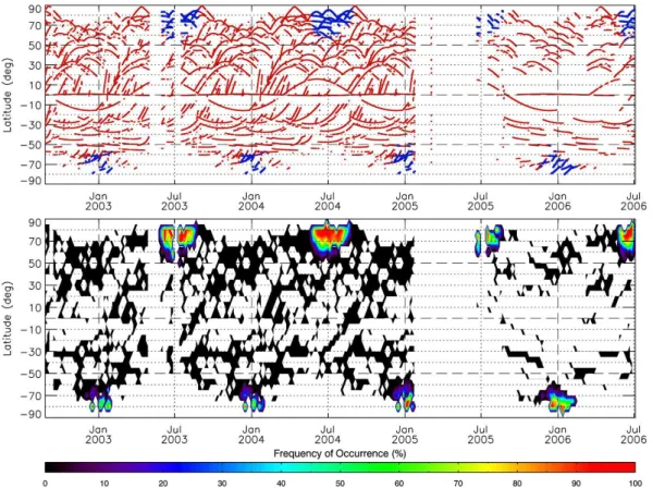
The finally obtained PMC data set can be summarized by Fig. 8. On the first plot, GOMOS observations are all repre-sented on the same figure. In this version, the latitude of the GOMOS measurements and of the observed clouds is plotted as a function of time all over the four years studied. The red and the blue symbols have the same meaning as in previous maps. This figure allows a very good visualization of the lat-itudinal coverage of the instrument. The measurements are spread over the entire globe, except in the Southern Hemi-sphere, where no dot appears at latitude below −80◦, as ex-plained in Sect. 2. A continuous red arc represents many occultations of the same star at successive orbits, covering all longitudes and slowly varying latitudes. We can check that noctilucent clouds are observed only at high latitudes in summer of both hemispheres. These results again show a significant amount of interannual variability in the temporal and latitudinal distribution of clouds observed by GOMOS. As told in Sect. 2, ENVISAT runs 14+11/35 orbits per day. The measurements are therefore very numerous and the blue dots, representing PMC detections, are sometimes superim-posed on the red ones. So this graph allows an accurate lo-cation of clouds on the globe and over the time, but does not allow distinguishing changes in their frequency.
As for Fig. 6, the second bottom plot represents the PMC detection frequency, but in this version it was calculated on a local level, in each square of 5 days by 5◦ of latitude. It appears that the presence of PMC is highly localized, both in time and in space. Their number varies very quickly: they ap-pear in the summer polar region and multiply in a few days.
29
Fig. 6. PMC detection frequency in 2-weeks time bins as a function of time all over the 4
years studied in the Northern Hemisphere (top) and in the Southern Hemisphere (bottom). Detection frequency is simply defined as the number of PMC detected in each 2-weeks period divided by the total number of GOMOS measurements in the same period, expressed in percent. Only the data situated in the latitude band ±[65; 75]° are considered here.
Fig. 6. PMC detection frequency in 2-weeks time bins as a function of time all over the 4 years studied in the Northern Hemisphere (top)
and in the Southern Hemisphere (bottom). Detection frequency is simply defined as the number of PMC detected in each 2-weeks period divided by the total number of GOMOS measurements in the same period, expressed in percent. Only the data situated in the latitude band
±65; 75◦are considered here.
Their frequency of occurrence tends to increase with latitude, to reach up to 100%. This is consistent with other PMC cli-matologies (Olivero and Thomas, 1986; Bailey, 2005). This figure highlights the fact that the south pole is less well ob-served than the north one. But, as previously noted, the mesospheric clouds still seem to be more frequent in the Northern Hemisphere than in the Southern Hemisphere, at the same latitude. The frequency values, here calculated on a local level, are more appropriate for interhemispheric com-parison. For a more quantitative comparison between the two hemispheres, various instrumental effects need to be taken into account. In particular different scattering angles (for-ward versus back(for-ward) lead to a difference in detected radi-ances and therefore also in frequencies of detection. In the case of GOMOS, the Southern Hemisphere is observed in a forward configuration (scattering angles from 40◦to 151◦), assumed more efficient for scattering of solar radiation, while the Northern Hemisphere is observed in a backward config-uration (scattering angles from 73◦to 180◦). Consequently, detection of the SH clouds is favored, and the differences between the hemispheres are therefore reduced by GOMOS viewing geometry.
These two plots show very well irregularities in GOMOS sampling frequency in both 2003 and 2005, as noticed
be-fore. Sparser GOMOS sampling in 2006 is also apparent. Fig. 7. Solid purple line: PMC detection frequency in 2-weeks time bins, in the latitude band ±[65; 75]° and combining the four years of data, for each hemisphere. Dotted-dashed lines: Total number of GOMOS measurements (in black) and of PMC observations (in blue). Time is expressed in days relative to summer solstice.
Fig. 7. Solid purple line: PMC detection frequency in 2-weeks time
bins, in the latitude band ±65; 75◦and combining the four years of data, for each hemisphere. Dotted-dashed lines: Total number of GOMOS measurements (in black) and of PMC observations (in blue). Time is expressed in days relative to summer solstice.
31
Fig. 8. Results of GOMOS data set analysis: General representation. Top: Observations
distribution as a function of time and latitude. As in Fig. 5, the red symbols represent all GOMOS measurements and the blue ones correspond to PMC detections. Bottom: PMC detection frequency as a function of time and latitude, calculated on a local level, in each square of 5 days by 5° of latitude. (In this figure, at highest latitudes observed, the frequency decreases, but is in fact always equal to 100%. This is only a bias due to the contour delineated algorithm.)
Fig. 8. Results of GOMOS data set analysis: General representation. Top: Observations distribution as a function of time and latitude. As
in Fig. 5, the red symbols represent all GOMOS measurements and the blue ones correspond to PMC detections. Bottom: PMC detection frequency as a function of time and latitude, calculated on a local level, in each square of 5 days by 5◦of latitude. (In this figure, at highest latitudes observed, the frequency decreases, but is in fact always equal to 100%. This is only a bias due to the contour delineated algorithm.)
4.4 PMC altitude determination
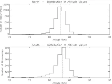
A PMC altitude data set was also produced, which is sum-marized on Fig. 9. The effective cloud height is defined as the tangent altitude corresponding to the highest peak of the signal. This altitude determination is correct only if the cloud layer is present at the line-of-sight tangent point and if it can be assumed to be approximately a simple spherical and uni-form shell. The cloud layers are spatially confined. Most of them are asymmetric about the tangent point, and this config-uration is not a problem, but in some cases, they do not cover the tangent point. Such cases produce misleading results. These cases correspond actually to events where the cloud was likely to have been detected entirely in the foreground or background along the line-of-sight. In this case, the deduced altitude will always be biased low. Indeed clouds sampled in this way do not yield a sharp, well defined peak in the intensity profile and are generally associated with very low altitude values. In order to eliminate them, all events where the obtained altitude was lower than 80 km were screened out, but it is possible that some errors remain.
In principle, the value deduced from both photometers should be identical. However, in practice, there are slight dif-ferences in some cases. The altitude was determined using the photometer which measures light in the blue, because, as previously noted, the effect of a PMC present along the line-of-sight is more marked in the blue wavelengths than in the red ones, but the second photometer was also used, in order to check the result. All cases where obtained values differ by more than 300 m were visually verified. Generally this problem occurs when one of the curves is wrong. So in these cases, one of the two values was chosen according to the shape of the curves.
95% of the obtained values range from 80 to 86 km, with a median value of 82.7 km in the North and 83.2 km in the
South. So mesospheric clouds are slightly higher in the
Southern Hemisphere, with a difference of about 500 m. These results are quite consistent with other measurements of PMC altitudes published in the literature. HALOE mea-surements yield a mean value of 83.3 km in the North and 84.2 km in the South (Wrotny and Russell, 2006). The mean altitude can also be derived from lidar: for example L¨ubken et al. (2008) have found a value of 83.3 km at ALOMAR (69◦N) and Chu et al. (2006) have found a value of 84.1 km
32
Fig. 9. Distribution of altitude values for each hemisphere. The obtained median value is
82.7km for the Northern Hemisphere and 83.2km for the Southern Hemisphere.
Fig. 9. Distribution of altitude values for each hemisphere. The
obtained median value is 82.7 km for the Northern Hemisphere and 83.2 km for the Southern Hemisphere.
at Rothera (67.5◦S). Collectively, the satellite and ground-based observations point to significant interhemispheric dif-ferences in PMC altitudes, with the southern clouds always higher than the northern ones. This can be explained by warmer temperatures in the South throughout the meso-sphere (Hervig and Siskind, 2006). The apparent discrep-ancy with GOMOS can be traced to different definitions of the considered PMC altitude. Most other studies use the al-titude corresponding to the maximum of brightness, or the centro¨ıd altitude (which is essentially the geometric center of the cloud layer), whereas the GOMOS cloud altitude is a tangent altitude, defined from brightness profiles integrated along the line of sight. The values obtained from this method are expected to be slightly lower than the true PMC altitudes. Limb observations of polar mesospheric clouds made from OSIRIS (Petelina et al., 2006) can be directly compared to the GOMOS measurements because the analyzed values are also tangent altitudes, observed in similar conditions. With a very close definition of the considered altitude, OSIRIS data yields a value of 82.3 km in the North and 83.4 km in the South, in agreement with GOMOS results.
This is only a first estimate of the PMC altitude. We plan to develop a cloud geometry model which will be able to fit the GOMOS PMC data. This simple inversion model will allow to carry out a more accurate study of PMC altitude and also to derive others geometric cloud parameters like the vertical thickness and the horizontal extent.
5 Summary and conclusions
This work yields a very rich PMC data set derived from the analysis of GOMOS photometers global observations. The technique of stellar occultation allows a very accurate alti-tude retrieval and a very good geographical and temporal coverage. For the moment 8 PMC seasons have been studied, from 2002 to 2006 in both hemispheres. A total of approx-imately 10 000 mesospheric clouds were detected all over these four years.
These results are summarized by a set of global maps which help us follow the evolution of clouds as a function of time and of their geographic location. Clouds appear over a period of approximately 70 days, with an occurrence fre-quency peaked about 20 days after summer solstice. There is a great deal of intrinsic interannual variability in the observed detection frequencies. The seasonally averaged frequencies calculated in 2-weeks time-bins in the latitude band ±65; 75◦range from about 10 to 80% in the Northern Hemisphere and from about 5 to 55% in the Southern Hemisphere dur-ing the PMC season, but reach 100% at high latitude when calculated at a local level, for both hemispheres. This shows that the PMC detection algorithm used for this analysis is very accurate, as it is able to detect even very faint clouds. These results agree reasonably well with other observations. They are one more piece of evidence that noctilucent clouds are more frequent in the North than in the South, although a further study is needed to make definite conclusions on the interhemispheric comparison. A PMC altitude data set was also produced, considering tangent altitudes. The obtained median value is 82.7 km for the Northern Hemisphere and 83.2 km for the Southern Hemisphere. So clouds are higher in the South, which is consistent with others studies made on this subject.
The algorithm described in this paper, which was de-veloped for the analysis of GOMOS photometers signals, yielded a very useful data set to study PMC, but it is still scarcely exploited. This work opens up many prospects, and will allow to conduct a comprehensive study of these myste-rious clouds at the edge of space. A vertical inversion will be performed to derive the main PMC characteristics (e.g. alti-tude, brightness, vertical thickness, geometric extent) and to study their variations. Extending these results to today and in the future will allow to obtain a long term data record, in order to better understand the link between these clouds and changes in their environment. Moreover the observa-tion of PMC with GOMOS spectrometers provides the spec-tral dependence of the scattering by these icy particles from which it is possible to derive some information on particle size. With this work, France is making its contribution in addressing the question of why noctilucent clouds form and vary.
Acknowledgements. This study was supported by the European
Space Agency, by the French funding agencies: INSU-CNRS and CNES, and by the European Commission within the SCOUT-03 project (contract 505390-GOCECT-2004).
Edited by: D. Murtagh
The publication of this article is financed by CNRS-INSU.
References
Bailey, S. M., Merkel, A. W., Thomas, G. E., and Carstens, J. N.: Observations of polar mesospheric clouds by the Stu-dent Nitric Oxide Explorer, J. Geophys. Res., 110, D13203, doi:10.1029/2004JD005422, 2005.
Baumgarten, G., Fiedler, J., and Von Cossart, G.: The size of noc-tilucent cloud particles above ALOMAR (69 N,16 E): Optical modeling and method description, Adv. Space Res., 40(6), 772– 784, 2007.
Berger, U. and L¨ubken, F.-J.: Weather in mesospheric ice layers, Geophys. Res. Lett., 33, L04806, doi:10.1029/2005GL024841, 2006.
Bertaux, J.-L., Hauchecorne, A., Dalaudier, F., Cot, C., Kyr¨ol¨a, E., Fussen, D., Tamminen, J., Leppelmeier, G. W., Sofieva, V., Hassinen, S., Fanton d’Andon, O., Barrot, G., Mangin, A., Th´eodore, B., Guirlet, M., Korablev, O., Snoeij, P., Koopman, R., and Fraisse, R.: First results on GOMOS/ENVISAT, Adv. Space Res., 33(7), 1029–1035, 2004.
Chu, X., Espy, P. J., Nott, G. J., Diettrich, J. C., and Gardner, C. S.: Polar mesospheric clouds observed by an iron Boltzmann li-dar at Rothera (67.5◦S, 68.0◦W), Antarctica from 2002 to 2005: properties and implications, J. Geophys. Res., 111, D20213, doi:10.1029/2006JD007086, 2006.
Collins, R. L., Bailey, S. M., Berger, U., L¨ubken, F.-J., and Merkel, A. W.: Special issue on global perspectives on the aeronomy of the summer mesopause region, J. Atmos. Sol.-Terr. Phy., 71(3– 4), 285–288, 2009.
Deland, M. T., Shettle, E. P., Thomas, G. E., and Olivero, J. J.: So-lar backscattered ultraviolet (SBUV) observations of poSo-lar meso-spheric clouds (PMCs) over two solar cycles, J. Geophys. Res., 108(D8), 8445, doi:10.1029/2002JD002398, 2003.
Deland, M. T., Shettle, E. P., Thomas, G. E., and Olivero, J. J.: A quarter-century of satellite PMC observations, J. Atmos. Sol-Terr. Phy., 68, 9–29, 2006.
Deland, M. T., Shettle, E. P., Thomas, G. E., and Olivero, J. J.: Latitude-dependent long-term variations in polar mesospheric clouds from SBUV version 3 PMC data, J. Geophys. Res., 112, D10315, doi:10.1029/2006JD007857, 2007.
Donahue, T. M., Guenther, B., and Blamont, J. E.: Noctilucent clouds in daytime: circumpolar particulate layers near the sum-mer mesopause, J. Atmos. Sci., 29(6), 1205–1209, 1972.
Envisat – GOMOS: An Instrument for Global Atmospheric Ozone Monitoring, ESA SP-1244, 2001.
Eremenko, M. N., Petelina, S. V., Zasetsky, A. Y., Karlsson, B., Rinsland, C. P., Llewellyn, E. J., and Sloan, J. J.: Shape and composition of PMC particles derived from satellite re-mote sensing measurements, Geophys. Res. Lett., 32, L16S06, doi:10.1029/2005GL023013, 2005.
Fiedler, J., Baumgarten, G., and von Cossart, G.: Mean diurnal vari-ations of noctilucent clouds during 7 years of lidar observvari-ations at ALOMAR, Ann. Geophys., 23, 1175–1181, 2005,
http://www.ann-geophys.net/23/1175/2005/.
Fiedler, J., Baumgarten, G., and L¨ubken, F.-J.: NLC observations during one solar cycle above ALOMAR, J. Atmos. Sol.-Terr. Phy., 71(3–4), 424–433, 2009.
Gerrard, A. J., Kane, T. J., Thayer, J. P., and Eckermann, S. D.: Con-cerning the upper stratospheric gravity wave and mesospheric cloud relationship over Søndrestrøm, Greenland, J. Atmos. Sol.-Terr. Phy., 66(3–4), 229–240, 2004.
Goldberg, R. A., Fritts, D. C., Schmidlin, F. J., Williams, B. P., Croskey, C. L., Mitchell, J. D., Friedrich, M., Russell III, J. M., Blum, U., and Fricke, K. H.: The MaCWAVE program to study gravity wave influences on the polar mesosphere, Ann. Geophys., 24, 1159–1173, 2006,
http://www.ann-geophys.net/24/1159/2006/.
Gumbel, J. and Witt, G.: In situ measurements of the vertical struc-ture of a noctilucent cloud, Geophys. Res. Lett., 25(4), 493–496, 1998.
Hansen, G., Serwazi, M., and Von Zahn, U.: First detection of a noctilucent cloud by lidar, Geophys. Res. Lett., 16, 1445–1448, 1989.
Hervig, M., Thompson, R. E., McHugh, M., Gordley, L. L., Russell III, J. M., and Summers, M. E.: First confirmation that water ice is the primary component of polar mesospheric clouds, Geophys. Res. Lett., 28(6), 971–974, 2001.
Hervig, M. and Siskind, D.: Decadal and inter-hemispheric variabil-ity in polar mesospheric clouds, water vapor, and temperature, J. Atmos. Sol.-Terr. Phy., 68(1), 30–41, 2006.
Karlsson, B., K¨ornich, H., and Gumbel, J.: Evidence for in-terhemispheric stratosphere-mesosphere coupling derived from noctilucent cloud properties, Geophys. Res. Lett., 34, L16806, doi:10.1029/2007GL030282, 2007.
Kyr¨ol¨a, E., Tamminen, J., Leppelmeier, G. W., Sofieva, V., Has-sinen, S., Bertaux, J.-L., Hauchecorne, A., Dalaudier, F., Cot, C., Korablev, O., Fanton d’Andon, O, Barrot, G., Mangin, A., Th´eodore, B., Guirlet, M., Etanchaud, F., Snoeij, P., Koopman, R., Saavedra, L., Fraisse, R., Fussen, D., and Vanhellemont, F.: GOMOS on Envisat: an overview, Adv. Space Res., 33(7), 1020– 1028, 2004.
Latteck, R., Singer, W., Morris, R. J., Holdsworth, D. A., and Murphy, D. J.: Observation of polar mesosphere summer echoes with calibrated VHF radars at 69◦ in the Northern and Southern Hemispheres, Geophys. Res. Lett., 34, L14805, doi:10.1029/2007GL030032, 2007.
Leslie, R.C.: Sky glows, Nature, 32, 245–245, doi:10.1038/032245a0., 1885.
L¨ubken, F.-J.: Thermal structure of the arctic summer mesosphere, J. Geophys. Res., 104(D8), 9135–9149, 1999.
L¨ubken, F.-J. and Berger, U.: Interhemispheric comparison of mesospheric ice layers from the LIMA model, J. Atmos. Sol.-Terr. Phy., 69(17–18), 2292–2308, 2007.
L¨ubken, F.-J., Baumgarten, G., Fiedler, J., Gerding, M., H¨offner, J., and Berger, U.: Seasonal and latitudinal variation of noc-tilucent cloud altitudes, Geophys. Res. Lett., 35, L06801, doi:10.1029/2007GL032281, 2008.
L¨ubken, F.-J., Berger, U., and Baumgarten, G.: Strato-spheric and solar cycle effects on long term variability of mesospheric ice clouds, J. Geophys. Res., 114, D00I06, doi:10.1029/2009JD012377, 2009.
Lumpe, J. D., Alfred, J. M., Shettle, E. P., and Bevilac-qua, R. M.: Ten years of Southern Hemisphere polar meso-spheric cloud observations from the Polar Ozone and Aerosol Measurement instruments, J. Geophys. Res., 113, D04205, doi:10.1029/2007JD009158, 2008.
Merkel, A. W., Thomas, G. E., Palo, S. E., and Bailey, S. M.: Obser-vations of the 5-day planetary wave in PMC measurements from the Student Nitric Oxide Explorer satellite, Geophys. Res. Lett., 30(4), 1196, doi:10.1029/2002GL016524, 2003.
Merkel, A. W., Marsh, D. R., Gettelman, A., and Jensen, E. J.: On the relationship of polar mesospheric cloud ice water content, particle radius and mesospheric temperature and its use in multi-dimensional models, Atmos. Chem. Phys., 9, 8889–8901, 2009, http://www.atmos-chem-phys.net/9/8889/2009/.
Murray, B. J. and Jensen, E. J.: Homogeneous nucleation of amor-phous solid water particles in the upper mesosphere, J. Atmos. Sol.-Terr. Phy., 72(1), 51–61, 2009.
Olivero, J. J. and Thomas, G. E.: Climatology of polar mesospheric clouds, J. Atmos. Sci., 43(12), 1263–1274, 1986.
Petelina, S. V., Llewellyn, E. J., Degenstein, D. A., and Lloyd, N. D.: Odin/OSIRIS limb observations of polar mesospheric clouds in 2001–2003, J. Atmos. Sol.-Terr. Phy., 68(1), 42–55, 2006. Robert, C. E., Von Savigny, C, Burrows, J. P., and Baumgarten, G.:
Climatology of noctilucent cloud radii and occurrence frequency using SCIAMACHY, J. Atmos. Sol.-Terr. Phy., 71(3–4), 408– 423, 2009.
Rusch, D. W., Thomas, G. E., and Jensen, E. J.: Particle size distributions in polar mesospheric clouds derived from Solar Mesosphere Explorer measurements, J. Geophys. Res., 96(D7), 12933–12939, 1991.
Russell, J. M. III, Bailey, S. M., Gordley, L. L., Rusch, D. W., Ho-ranyi, M., Hervig, M. E., Thomas, G. E., Randall C. E., Siskind, D. E., Stevens, M. H., Summers, M. E., Taylor, M. J., Englert, C. R., Espy, P. J., McClintock, W. E., and Merkel, A. W.: The Aeronomy of Ice in the Mesosphere (AIM) mission: overview and early science results, J. Atmos. Sol.-Terr. Phy., 71(3–4), 289– 299, 2009.
Shettle, E. P., Deland, M. T., Thomas, G. E., and Olivero, J. J.: Long term variations in the frequency of polar mesospheric clouds in the Northern Hemisphere from SBUV, Geophys. Res. Lett., 36, L02803, doi:10.1029/2008GL036048, 2009.
Stevens, M. H., Englert, C. R., Hervig, M., Petelina, S. V., Singer, W., and Nielsen, K.: The diurnal variation of polar mesospheric cloud frequency near 55◦N observed by SHIMMER, J. Atmos. Sol.-Terr. Phy., 71(3–4), 401–407, 2009.
Sonnemann, G. R. and Grygalashvyly, M.: Solar influence on meso-spheric water vapor with impact on NLCs, J. Atmos. Sol.-Terr. Phy., 67(1–2), 177–190, 2005.
Taylor, M. J., Gadsden, M., Lowe, R. P., Zalcik, M. S., and Brausch, J.: Mesospheric cloud observations at unusually low latitudes, J. Atmos. Sol.-Terr. Phy., 64, 991–999, 2002.
Thayer, J. P., Rapp, M., Gerrard, A. G., Gudmundsson, E., and Kane, T. J.: Gravity-wave influences on Arctic mesospheric clouds as determined by a Rayleigh lidar at Søndrestrøm, Greenland, J. Geophys. Res., 108(D8), 8449, doi:10.1029/2002JD002363, 2003.
Thomas, G. E., Olivero, J. J., Jensen, E. J., Schroeder, W., and Toon, O. B.: Relation between increasing methane and the presence of ice at the mesopause, Nature, 338, 490–492, 1989.
Thomas, G. E., McPeters, R. D., and Jensen, E. J.: Satellite obser-vations of polar mesospheric clouds by the Solar Backscattered Ultraviolet spectral radiometer: evidence of a solar-cycle depen-dence, J. Geophys. Res., 96(D1), 927–939, 1991.
Thomas, G. E. and Olivero, J. J.: Noctilucent clouds as possible indicators of global change in the mesosphere, Adv. Space Res., 28(7), 937–946, 2001.
Thomas, G. E., Olivero, J. J., Deland, M. T., and Shettle, E. P.: Comment on “Are noctilucent clouds truly a ‘miner’s canary’ for global change?”, EOS, Transactions American Geophysical Union, 84(36), doi:10.1029/2003EO360008, 2003.
Von Savigny, C., Petelina, S. V., Karlsson, B., Llewellyn, E. J., Degenstein, D. A., Lloyd, N. D., and Burrows, J. P.: Verti-cal variation of NLC particle sizes retrieved from Odin/OSIRIS limb scattering observations, Geophys. Res. Lett., 32, L07806, doi:10.1029/2004GL021982, 2005.
Von Zahn, U.: Are noctilucent clouds truly a “miner’s canary” of global change?, EOS, Transactions American Geophysical Union, 84(28), doi:10.1029/2003EO280001, 2003.
W¨alchli, U., Stegman, J., Witt, G., Cho, J. Y. N., Miller, C. A., Kelley, M. C., and Swartz, W. E.: First height comparison of noctilucent clouds and simultaneous PMSE, Geophys. Res. Lett., 20(24), 2845–2848, 1993.
Wrotny, J. E. and Russell III, J. M.: Interhemispheric differences in polar mesospheric clouds observed by the HALOE instrument, J. Atmos. Sol.-Terr. Phy., 68(12), 1352–1369, 2006.
Zasetsky, A. Y., Petelina, S. V., and Svishchev, I. M.: Thermody-namics of homogeneous nucleation of ice particles in the polar summer mesosphere, Atmos. Chem. Phys., 9, 965–971, 2009a, http://www.atmos-chem-phys.net/9/965/2009/.
Zasetsky, A. Y., Petelina, S. V., Remorov, R., Boone, C. D., Bernath, P. F., and Llewellyn, E. J.: Ice particle growth in the polar sum-mer mesosphere: Formation time and equilibrium size, Geophys. Res. Lett., 36, L15803, doi:10.1029/2009GL038727, 2009 b.