Small-scale spatial structure in plankton distributions

HAL Id: hal-00297857

https://hal.archives-ouvertes.fr/hal-00297857

HAL is a multi-disciplinary open access

archive for the deposit and dissemination of sci-entific research documents, whether they are pub-lished or not. The documents may come from teaching and research institutions in France or abroad, or from public or private research centers.

L’archive ouverte pluridisciplinaire HAL, est destinée au dépôt et à la diffusion de documents scientifiques de niveau recherche, publiés ou non, émanant des établissements d’enseignement et de recherche français ou étrangers, des laboratoires publics ou privés.

Small-scale spatial structure in plankton distributions

A. Tzella, P. H. Haynes

To cite this version:

A. Tzella, P. H. Haynes. Small-scale spatial structure in plankton distributions. Biogeosciences Dis-cussions, European Geosciences Union, 2006, 3 (6), pp.1791-1808. �hal-00297857�

BGD

Full Screen / Esc

Printer-friendly Version Interactive Discussion Biogeosciences Discuss., 3, 1791–1808, 2006

www.biogeosciences-discuss.net/3/1791/2006/ © Author(s) 2006. This work is licensed

under a Creative Commons License.

Biogeosciences Discussions

Biogeosciences Discussions is the access reviewed discussion forum of Biogeosciences

Small-scale spatial structure in plankton

distributions

A. Tzella and P. H. Haynes

Department of Applied Mathematics and Theoretical Physics, University of Cambridge, UK Received: 31 October 2006 – Accepted: 26 November 2006 – Published: 4 December 2006 Correspondence to: A. Tzella ([email protected])

BGD

Full Screen / Esc

Printer-friendly Version Interactive Discussion

Abstract

The observed filamental nature of plankton populations suggests that stirring plays an important role in determining their spatial structure. If diffusive mixing is neglected, the various interacting biological species within a fluid parcel are determined by the parcel time history. The induced spatial structure has been shown to be a result of competition

5

between the time evolution of the biological processes involved and the stirring induced by the flow as measured, for example, by the rate of divergence of the distance of neigh-bouring fluid parcels. In the work presented here we examine a simple biological model based on delay-differential equations, previously seen inAbraham(1998), including nu-trients, phytoplankton and zooplankton, coupled to a strain flow. Previous theoretical

10

investigations made on a differential equation model (Hern ´andez-Garcia et al.,2002) imply that the latter two should share the same small-scale structure. The general-ization from differential equations to delay-differential equations, associated with the addition of a maturation time to the zooplankton growth, should not make a difference, provided sufficiently small spatial scales are considered. However, this theoretical

pre-15

diction is in contradiction with the results ofAbraham(1998), where the phytoplankton and zooplankton structures remain uncorrelated at all length scales. A new set of nu-merical experiments is performed here which show that these two regimes coexist. On larger scales , there is a decoupling of the spatial structure of the zooplankton distri-bution on the one hand, and the phytoplankton and nutrient on the other. On the other

20

hand, at small enough length scales, the phytoplankton and zooplankton share the same spatial structure as expected by the theory involving no maturation time.

1 Introduction

The generation of patchiness in planktonic distributions is a result of the biological in-teractions between species coupled to the background fluid motion. Phytoplankton

25

distributions during springtime blooms, a consequence of ocean stratification and sea-1792

BGD

Full Screen / Esc

Printer-friendly Version Interactive Discussion sonal increase in sunlight, are strongly inhomogeneous and filamental with structures

that range from 1 to 100 km. Moreover, these distributions exhibit similar power law spectra to physical quantities like sea surface temperature (Seuront et al.,1996,1999). On the other hand, most observations of patchiness in zooplankton indicate a flatter or noisier spectrum than the phytoplankton (Tsuda et al., 1993), though, this result has

5

been questioned byMartin and Srokosz(2002). For a review seeMartin(2003). The phytoplankton filaments observed in colour satellite images are mostly formed in the strain-dominated regions of the ocean between mesoscale eddies or along fronts. At these scales, oceanic turbulence is now understood to be strongly anisotropic (McWilliams et al., 1994), dominated by the directional activity of these eddies and

10

fronts. Consequently, models employing eddy diffusion in order to parametrize turbu-lence and explain patchiness (Okubo,1971), are rendered irrelevant at the mesoscale. Instead, it is advection which plays an important role in their formation.

Unlike eddy diffusion, advection is responsible for the transfer of large-scale inho-mogeneities into smaller scales. Such a transfer from the larger scales (∼100 km) has

15

been shown numerically to take approximately 10 days to reach∼1 km at which point three-dimensional flow becomes important (Klein and Hua,1990). This is less than the maturation time of zooplankton such as copepods which is typically 25 days (Kiorboe and Sabatini, 1995). This means that during their lifetime, any large-scale variation (e.g.∼100 km) will be stirred down to kilometre lengths.

20

It has been previously recognized (e.g. Haynes,1999) that the dominant contribu-tion to adveccontribu-tion in large scale stably stratified geophysical flows can be successfully captured by two-dimensional spatially smooth and time-dependent velocity fields, that generate chaotic trajectories for the fluid particles. This chaotic advection (Aref,1984), leads to small-scale structures in inert tracers. It turns out that a number of explicit

25

results are insensitive to the model’s details. It is sufficient to know the ability of a flow to mix with a tracer, measured by the rate at which fluid parcel trajectories diverge from each other (Ottino,1989). At scales larger than the mixed-layer turbulence scale of a few hundred meters the effects of molecular diffusion can be neglected and the

BGD

Full Screen / Esc

Printer-friendly Version Interactive Discussion logical properties within a fluid parcel can be considered to evolve independently of its

surroundings. Hence, the concentrations of different planktonic species can be taken to be uniformly distributed within a fluid parcel and determined by the time history of that parcel.

The emergence of persistent patterns requires some spatially varying external

forc-5

ing such as a localised upwelling of nutrients or a latitudinal variation of sunlight. The induced spatial structure has been shown to be a result of competition between the rate of convergence of the biological processes involved and the rate of divergence of the distance of neighbouring fluid parcels. It has also been argued that, except under rather special conditions, the small scale behaviour should be the same for all

inter-10

acting species (Neufeld et al.,1999; Hern ´andez-Garcia et al.,2001,2002). However Abraham (1998) has presented results for a system in which the biological evolution equations include a maturation time for the zooplankton growth that results in a different small-scale spatial structure for the phytoplankton and the zooplankton, in disagree-ment with the case of a zero maturation time. This inclusion transforms the original set

15

of ordinary differential equations to a set of delay differential equations.

In this work we examine a class of models involving a nutrient, a prey and a predator, in order to represent the interactions between nutrient phytoplankton and zooplankton species, known as the NPZ models (Hern ´andez-Garcia et al.,2001). These are cou-pled to the flow by a spatially inhomogeneous forcing. A natural way to characterize

20

the emerging spatial distributions is to investigate the scaling properties of statistical quantities such as Fourier power spectra or structure functions of the corresponding concentration fields. A set of numerical simulations are in good agreement with the re-sults attained byNeufeld et al.(1999). The inclusion of a maturation time changes the differential equations that govern the interacting species to delay differential equations.

25

Although this is a significant alteration, the essential conclusions regarding the be-haviour of the structure functions remain unchanged, provided sufficiently small scales are considered. However, there appears to be a decoupling of the spatial structure of zooplankton on the one hand and phytoplankton and nutrient on the other, at scales

BGD

Full Screen / Esc

Printer-friendly Version Interactive Discussion larger than a particular characteristic length scale. This result reconciles the

contra-dicting conclusions given byNeufeld et al.(1999) andAbraham(1998).

2 Biological-fluid coupling

In the numerical investigations undertaken, we will assume that the flow v(x, t) is two-dimensional and incompressible. These conditions are usually enough to ensure the

5

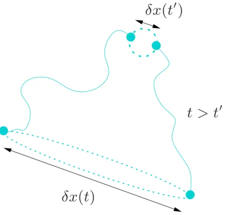
chaotic advection of fluid parcels, even if the velocity field is a smooth function of space (Ottino,1989). A way to characterize the flow is to look at its Lyapunov exponent,λ_F, defined as the exponential rate of separation of initially neighbouring fluid particles (Fig.1). Since the fluid is incompressible, its volume must be conserved, and therefore contraction must take place in another direction. Moreover, the contraction and also the

10

expansion occur at the same exponential rateλ_F. Consequently, blobs of fluid stretch along long and thin filaments and are repeatedly folded, thus transferring large-scale inhomogeneities into smaller ones.

Although the detailed flow used byAbraham(1998) was different, the essential points characterizing the strain dominated regions between the eddy regions is captured by

15

the flow used here. The domain of the velocity field is taken to be a periodic square with side lengthL, approximately 50 km, corresponding to the characteristic lengthscale of a mesoscale eddy. It will represent the regions that are formed between large eddies, where the phytoplankton filaments are usually observed. This is a pure strain velocity field whose form is

20 v(x, t) =      −2 TΘ(T/2 − t mod T ) cos(2πy/L + φ) −2 TΘ(t modT − T/2) cos(2πx/L + θ)      , (1)

where Θ(t) is the Heaviside step function defined to be equal to unity for t≥0 and zero otherwise. The phase anglesθ and φ change randomly at each period T of the flow,

BGD

Full Screen / Esc

Printer-friendly Version Interactive Discussion varying the directions of expansion and contraction and hence ensuring all parts of it

are equally mixed (Bohr et al., 1998; Ott,1993). Variation of T has an effect on the magnitude ofλ_F without changing the shape of the trajectories and spatial structure of the flow.

A number of independent fluid parcels are advected by this velocity field. Each one

5

of them carries a uniform distribution of phytoplanktonP and zooplankton Z, the latter applied mostly to copepod species, as these can be assumed to be drifting with their respective fluid parcels. On the other hand, large zooplankton, such as krill, actively modify their distributions by swimming (Trathan et al.,1993).

The interactions among the biological species are described in a model already

10

employed by Abraham (1998). This is a typical nutrient-predator-prey system ( Mur-ray,1993), where the former is parametrized by the carrying capacity C of the fluid parcel, defined as the maximum phytoplankton content that the parcel can sup-port in the absence of grazing. As the fluid parcel moves through the domain, the carrying capacity continuously relaxes to a space varying background source,

15

C0(x, y)=(1−cos(2π(x +y)/L)), where x and y are the domain’s horizontal and vertical

axes respectively. A large scale inhomogeneity is thus introduced into the system. The species’ dynamics are described by the following dimensionless equations, d C d t =α(C0(x)− C), (2a) d P d t =P (1 − P/C) − P Z, (2b) 20 dZ d t =P (t − τ)Z(t − τ) − δZ 2_, (2c) where t is the dimensionless time scaled to the phytoplankton production rate r=0.5d−1(t/r is the real time), α denotes the rate at which the carrying capacity relaxes to the background sourceC0, δ is the zooplankton mortality rate and τ/r represents

the time taken for the zooplankton to mature. Although it is plausible to assume an

25

instantaneous change in the prey population once prey and predator are encountered, 1796

BGD

Full Screen / Esc

Printer-friendly Version Interactive Discussion it is not reasonable to assume an instantaneous change in the predator population,

and this is the motivation behind the employment of this maturation time.

The phytoplankton growth is logistic and the grazing takes place according to a sim-pleP Z term. In the absence of advection, C0(x) is a constant, since the parcel

posi-tion remains unchanged, and the only fixed point of the model is given byC⋆=_C

0(x),

5

P⋆=_{δC0/(δ+C0) andZ}⋆=_P⋆_{/δ. This point is a stable fixed point of equilibrium for τ=0,} meaning that any perturbation around this point will eventually decay to zero. IfC0≤1

andδ≥0.5, as in the simulations performed here, it remains stable for any maturation time.

In the presence of the sourceC0(x), this equilibrium point can never be reached due

10

to the continually varying carrying capacity within the fluid parcel. The continual input of large-scale inhomogeneites injected by C0(x) and their transfer to smaller scales

by advection leads to a non-trivial statistical steady state. The study of the induced complex patterns will be the focus of the next sections.

3 Methodology

15

The planktonic distributions at a particular time are reconstructed by following an en-semble of fluid parcels. In the method used byAbraham (1998), the fluid parcels are tracked forwards in time and the corresponding distributions are obtained from a De-launay triangulation of the parcel positions by linear interpolation onto a regular grid. Here, the parcels final positions are fixed to a grid. The parcels are then tracked

back-20

wards in time up to a time when their initial biological concentration fields are known. Thereafter, knowing their trajectory, their biological evolution is determined by integrat-ing along this trajectory up to the final time usintegrat-ing a second order Runge-Kutta method. This way, no interpolation is necessary and consequently greater accuracy at smaller length scales is achieved. For the concentrations to be accurate up to three decimal

25

places, the timestep is chosen to be 0.001. This value in real time corresponds to 0.002d−1 and is in line with the assumption made of uniformly distributed populations

BGD

Full Screen / Esc

Printer-friendly Version Interactive Discussion within the fluid parcels. The ensemble of fluid parcels considered here is 250 000 and

evenly spans a grid of resolution 500×500. Their initial concentrations are set to be equal to their mean equilibrium values.

A statistical steady state is reached after 20T , where T is the period of the flow. The emerging patterns are complex in space (Fig.3). The standard way to characterize

5

such structures is by their Fourier power spectra. Here, we will also consider their first-order structure function (Monin and Yaglom, 1975), the square root of the variance, defined by

S(δx) ≡ h|c(x + δx) − c(x)|i ∼ (δx)γ, (3)

whereh...i denotes averaging over different values of the coordinate x. The scaling

10

exponent,γ, known as the H ¨older exponent, is related to the power spectrum exponent, ǫ, by the simple relationship ǫ=1+2γ, where 0<γ<1 corresponds to a rough structure andγ=1 to a smooth one.

4 Numerical results

The emergent spatial structures depend on the relative strength of the dispersion of the

15

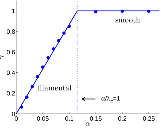
parcel trajectories and the stability of the biological dynamics. The phytoplankton car-rying capacity, whose biological evolution is described by Eq. (2a), has a structure that has been shown inNeufeld et al.(1999) to be characterized by two types of behaviour that depend on the interplay between the relaxation rateα and the Lyapunov exponent λF. Ifα>λF, the biological processes converge faster to their equilibrium value than

20

the trajectories diverge from each other. The corresponding distribution is smooth. On the other hand, ifα<λ_F, the biological processes are too slow to forget the different spatial histories experienced by the parcels. The corresponding distribution is rough, with a H ¨older exponentγ=α/λF in all directions except for the one that the filaments

grow into. This type of structure has been defined byNeufeld et al.(1999) as

filamen-25

tal. The transition from a filamental to a smooth structure asα varies is depicted in 1798

BGD

Full Screen / Esc

Printer-friendly Version Interactive Discussion Fig.2. The numerical agreement with the theoretical prediction gives confidence in the

method used here.

As inAbraham(1998),α is taken to be equal to 0.25 corresponding to a tracer that takes 8d to adapt to a background force. Choosing a flow withλ_F∼0.11 (achieved by setting the period to T =20), the emerging phytoplankton carrying capacity structure

5

is smooth. This is similar to physical quantities such as the sea surface temperature whose spectral slope has been measured to beǫ=3, equivalent to γ=1 (Deschamps et al.,1981). The limit ofα tending to zero corresponds to a tracer that takes an infinite time to adapt to a background source, i.e. a passive non-reactive tracer. Its expected exponent in a two-dimensional turbulent flow isǫ=1 or γ=0 (Powell and Okubo,1994).

10

The above suggests that although the model considered is simple, it is adequate to de-scribe the transfer of variability to smaller scales and hence capture the basic features of turbulence. Moreover, the exact details of the flow are not important as long as the fluid parcels are chaotically advected.

For a general biological system, the same smooth filamental transition can be

ob-15

tained. A system similar to the one described in Eq. (2), in the absence of a maturation time (τ=0), has previously been examined in Hern ´andez-Garcia et al. (2002). In this case, the phytoplankton and zooplankton populations always share the same small-scale structure. This is not the case for the carrying capacity, due solely to it not being symmetricaly coupled to the rest of the populations.

20

Using the same flow as before, a new set of numerical experiments is carried out, with the same biological parameters used byAbraham(1998). Because of the numer-ical method used, higher spatial resolution can be achieved. Here, the length scales considered reach 0.002 L, (∼100 m, the scale at which turbulence ceases to be two-dimensional). The induced spatial patterns can be seen in Fig.3. At first sight, the

25

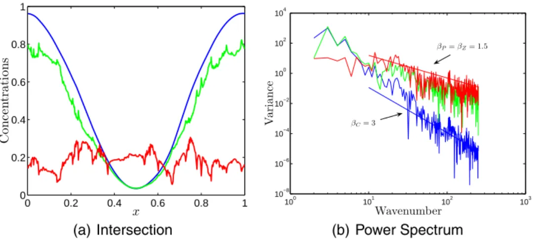
phytoplankton and zooplankton populations seem to be decoupled at all length scales, comfirming the picture given by Abraham (1998). However, a transect through the model domain (Fig.4(a)), shows that at small enough length scales, both phytoplank-ton and zooplankphytoplank-ton exhibit a fine scale structure. Their corresponding power spectra

BGD

Full Screen / Esc

Printer-friendly Version Interactive Discussion (Fig.4(b)), reveal that at large wavelengths (k>10/L∼0.2km−1), they share the same

structure with a spectral exponent larger than 1. As expected, the carrying capacity behaves smoothly at all scales. At smaller wavelengths, corresponding to larger length scales, the picture provided by Abraham (1998) is recovered with the phytoplankton spectral slope steepening and the zooplankton one flattening out.

5

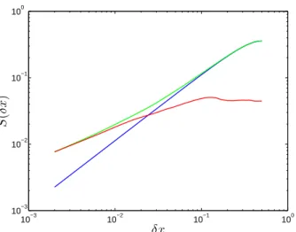
Perhaps a better way to picture this transition is by looking at the corresponding first-order structure functions as the length scaleδx increases (Fig. 5). For δx<δx_c, whereδx_c is a characteristic lengthscale approximately equal to 10−2L(∼ 5 km), the phytoplankton and zooplankton share similar structures. As δx increases, there is a regime change where the phytoplankton population decouples from the zooplankton

10

population. At this point the phytoplankton acquires a similar distribution to the carrying capacity, while the zooplankton distribution becomes increasingly flat.

5 Conclusions

The small-scale structure of interacting nutrient, phytoplankton and zooplankton pop-ulations, passively advected by a two-dimensional flow and coupled to it through an

15

inhomogeneous source, is here discussed. The particular focus is on the effect in-duced in these structures by introducing a maturation time in the zooplankton growth.

According to Hern ´andez-Garcia et al. (2002), given a particular class of flow and in the absence of a maturation time, the small-scale structure for the phytoplankton and zooplankton should be the same , given that they are symmetrically coupled, and

20

characterized by a single exponent at all small scales. The inclusion of a maturation time,τ, should not alter the above conclusions. Although the nature of the equations changes from ordinary to delay, there still exists a set of biological decay rates, shared by the phytoplankton and the zooplankton, that should dictate their common structure at small enough scales. This is in disagreement with the numerical results obtained

25

in Abraham (1998). There, the phytoplankton and the carrying capacity turn out to have similar distributions, close to a smooth one and completely decoupled to the

BGD

Full Screen / Esc

Printer-friendly Version Interactive Discussion zooplankton’s. As τ increases, the zooplankton’s distribution becomes increasingly

filamental, ultimately behaving like a passive tracer (β → 1 or γ → 0). The aim of this work has been to resolve this disagreement.

Using a model flow to depict the strain dominated regions formed between mesoscale eddies, we reproduce the regime observed byAbraham(1998). However,

5

the alternative numerical method used here permits the study of smaller length scales where it is revealed that this is only part of the true picture: as long as small enough length scales are considered, a second regime appears where the phytoplankton and zooplankton distributions share the same small-scale structure. The transition between these two regimes occurs at a characteristic length scale.

10

Hence, by introducing a maturation time, both the phytoplankton and zooplankton structures can no longer be characterized by a single exponent at all scales smaller than that of the flow. Perhaps this point, along with the shared exponent at small enough length scales, should be taken into account in trying to interpret observa-tional measurements in phytoplankton and zooplankton distributions at a large range

15

of length scales.

The conditions under which the decoupling of zooplankton and phytoplankton take place are still not completely understood. The effect the biological and the flow activ-ity have on the characteristic length size of the plankton distributions is the subject of current theoretical investigations that will be reported elsewhere. While many issues

20

remain to be resolved, it is hoped that the present paper will provide another step to-wards understanding the complicated dynamics of plankton in the presence of oceanic fluid motions.

References

Abraham, E. R.: The generation of plankton patchiness by turbulent stirring, Nature, 391, 577–

25

580, 1998.1792,1794,1795,1796,1797,1799,1800,1801

Aref, H.: Stirring by chaotic advection, J. Fluid Mech., 143, 1, 1984. 1793

BGD

Full Screen / Esc

Printer-friendly Version Interactive Discussion

Bohr, T., Jensen, M., Paladin, G., and Vulpiani, A.: Dynamical Systems Approach to Turbulence, Cambridge University Press, Cambridge, 1998. 1796

Deschamps, P., Frouin, R., and Wald, L.: Satellite determinations of the mesoscale variability of the sea surface temperature, J. Phys. Oceanogr., 11, 864–870, 1981. 1799

Haynes, P. H.: Transport, stirring an mixing in the atmosphere in Mixing – Chaos and

turbu-5

lence, edited by: Chate, H., Villermaux, E., and Chomaz, J. M., Kluwer, Dordretch, 1999. 1793

Hern ´andez-Garcia, E., L ´opez, C., and Neufeld, Z.: Spatial patterns in chemically and bio-logically reacting flows, Chaos in Geophysical Flows, edited by: Boffetta, G., Lacorata, G., Visconti, G., and Vulpiani, A., OTTO editore (Torino), 2001. 1794

10

Hern ´andez-Garcia, E., L ´opez, C., and Neufeld, Z.: Small-scale structure of nonlinearly inter-acting species advected by chaotic flows, CHAOS, 12, 470, 2002.1792,1794,1799,1800 Kiorboe, T. and Sabatini, M.: 1995 Scaling and fecundity, growth and development in marine

planktonic copepods., Mar. Ecol. Prog. Ser., 120, 285–298, 1995. 1793

Klein, P. and Hua, B. L.: The mesoscale variability of the sea surface temperature: An analytical

15

and numerical model, J. Mar. Res., 48, 729–763, 1990. 1793

Martin, A. P.: Phytoplankton patchiness: the role of lateral stirring and mixing, Prog. Oceanogr., 57, 125–174, 2003.1793

Martin, A. P. and Srokosz, M. A.: Plankton distribution spectra: inter-size class variability and the relative slopes for phytoplankton and zooplankton., Geophys. Res. Lett., 29, 2213,

20

doi:10.1029/2002GL015117, 2002. 1793

McWilliams, J., Weiss, J., and Yavneh, I.: Anisotropy and coherent vortex structures in planetary turbulence, Science, 264, 410–413, 1994. 1793

Monin, A. S. and Yaglom, A. M.: Statistical Fluid Mechanics, MIT Press, Cambridge, 1975. 1798

25

Murray, J. D.: Mathematical Biology, Springer-Verlag, New York, 1993.1796

Neufeld, Z., L ´opez, C., and Haynes, P. H.: Smooth-Filamental Transition of Active Tracer Fields Stirred by Chaotic Advection, Phys. Rev. Lett., 82, 2606–2609, 1999. 1794,1795,1798 Okubo, A.: Oceanic diffusion diagrams., Deep-Sea Res., 18, 789–802, 1971.1793

Ott, E.: Chaos in Dynamical Systems, Cambridge University Press, Cambridge, 1993.1796

30

Ottino, J. M.: The kinematics of mixing: Stretching, chaos and transport., Cambridge University Press, Cambridge, 1989. 1793,1795

Powell, T. M. and Okubo, A.: Turbulence diffusion and patchiness in the sea, Phil. Trans. R.

BGD

Full Screen / Esc

Printer-friendly Version Interactive Discussion

Soc. Lond. B, 343, 11–18, 1994. 1799

Seuront, L., Schmitt, F., Lagadeuc, Y., Schertzer, D., Lovejoy, S., and Frontier, S.: Multifractal analysis of phytoplankton biomass and temperature in the ocean., Geophys. Res. Lett., 23, 3591–3594, 1996. 1793

Seuront, L., Schmitt, F., Lagadeuc, Y., Schertzer, D., and Lovejoy, S.: Universal multifractal

5

analysis as a tool to characterize multiscale intermittent patterns: example of phytoplankton distribution in turbulent coastal waters., J. Plankton Res., 21, 977–922, 1999. 1793

Trathan, P. N., Priddle, J., Watkins, J. L., Miller, D. G. M., and Murray, A. W. A.: Spatial variabiity of Antarctic krill in relation to mesoscale hydrography., Mar. Ecol. Prog. Ser., 98, 61–71, 1993. 1796

10

Tsuda, A., Sugisaki, H., Ishimoru, T., Saino, T., and Sato, T.: White-noise-like distribution of the oceanic copepod Neocalanus cristatus in the subarctic North Pacific., Mar. Ecol. Prog. Ser., 97, 39–46, 1993. 1793

BGD

Full Screen / Esc

Printer-friendly Version Interactive Discussion

eities into smaller ones.

0

1 0

1

δx

_(t

′

₎

δx

_(t)

t > t

′

Fig. 1. Set of trajectories for a pair of fluid parcels. evolving either forwards (t>t′) or back-wards (t<t′) in time. Their separation is dominated by an exponential behaviour such that

δx(t)∼eλF(t−t′)_δx(t′_{), where λ}

F is the Lyapunov exponent of the flow. The dotted lines

repre-sent the stretching of a blob of fluid into a filament by the flow.

BGD

Full Screen / Esc

Printer-friendly Version Interactive Discussion

0

0.05

0.1

0.15

0.2

0.25

0

0.2

0.4

0.6

0.8

1

α

γ

α

_/

λ

=1

filamental

smooth

Fig. 2. Variation of the small-scale structure for the phytoplankton carrying capacity in response

to the rateα, at which it relaxes towards a smoothly varying background source. The structure

is characterized by the H ¨older exponent,γ, whose value depends on the ratio of α over the

Lyapunov exponentλ_F. When this ratio is bigger than 1 the corresponding structure is smooth otherwise it is filamental. The dots mark γ averaged over 500 evenly spaced intersections,

while the straight line represents its theoretical value. During this set of experiments,λ_F∼0.11.

BGD

Full Screen / Esc

Printer-friendly Version Interactive Discussion x y 0.2 0.4 0.6 0.8 1 0.2 0.4 0.6 0.8 1 0.1 0.2 0.3 0.4 0.5 0.6 0.7 0.8 0.9

(a) Carrying capacity

x y 0.2 0.4 0.6 0.8 1 0.2 0.4 0.6 0.8 1 0.1 0.2 0.3 0.4 0.5 0.6 0.7 0.8 (b) Phytoplankton x y 0.2 0.4 0.6 0.8 1 0.2 0.4 0.6 0.8 1 0.05 0.1 0.15 0.2 0.25 0.3 (c) Zooplankton

Fig. 3. Snapshots of the biological distributions at statistical equilibrium (t=20T ). The model

follows Eq. (2) withτ/r=25d and δ=2, denoting a high mortality zooplankton regime. The

smoothly varying forceC₀(x, y)=(1 − cos(2π(x+y)/L)) is diagonally oriented. The bar on the

right gives the concentration values associated with the different colours. The flow is described in Eq. (1) where the periodT =20. The axes are measured in units of L, where L is

approxi-mately 50 km.

BGD

Full Screen / Esc

Printer-friendly Version Interactive Discussion 0 0.2 0.4 0.6 0.8 1 0 0.2 0.4 0.6 0.8 1 x C o n c e n t r a t io n s (a) Intersection 100 101 102 103 10−8 10−6 10−4 10−2 100 102 104 Wavenumber V a r ian c e βP=βZ= 1.5 βC= 3 (b) Power Spectrum

Fig. 4. A representative transect (aty=0.5 L) and the corresponding spectra. Graphs show

carrying capacity (blue), phytoplankton (green) and zooplankton (red). The spectra are ob-tained over 500 evenly spaced horizontal transects and have a power law form. The spectral exponents of the populations areβ_C=3 andβ_P=_β

Z=1.5 The horizontal axes are measured in

units of lengthL and wavenumber 1/L respectively .

BGD

Full Screen / Esc

Printer-friendly Version Interactive Discussion 10−3 10−2 10−1 100 10−3 10−2 10−1 100 δx S ( δ x)

Fig. 5. First-order structure functions averaged over 500 evenly spaced horizontal transects.

Graph shows carrying capacity (blue), phytoplankton (green) and zooplankton (red). The hor-izontal axes are measured in units of lengthL. The H ¨older exponent of the carrying capacity

isγ_C=1. The phytoplankton and zooplankton respective exponents vary withδx. For δx<δx_c, whereδx_c≈ 10−2L, γ_P=_γ

Z=0.5. For δx>δxc,γC=γP=1 andγZ=0.