HAL Id: hal-00297605
https://hal.archives-ouvertes.fr/hal-00297605
Submitted on 2 Mar 2007
HAL is a multi-disciplinary open access
archive for the deposit and dissemination of
sci-entific research documents, whether they are
pub-lished or not. The documents may come from
teaching and research institutions in France or
abroad, or from public or private research centers.
L’archive ouverte pluridisciplinaire HAL, est
destinée au dépôt et à la diffusion de documents
scientifiques de niveau recherche, publiés ou non,
émanant des établissements d’enseignement et de
recherche français ou étrangers, des laboratoires
publics ou privés.
Small-scale spatial structure in plankton distributions
A. Tzella, P. H. Haynes
To cite this version:
A. Tzella, P. H. Haynes. Small-scale spatial structure in plankton distributions. Biogeosciences,
European Geosciences Union, 2007, 4 (2), pp.173-179. �hal-00297605�
www.biogeosciences.net/4/173/2007/ © Author(s) 2007. This work is licensed under a Creative Commons License.
Biogeosciences
Small-scale spatial structure in plankton distributions
A. Tzella and P. H. Haynes
Department of Applied Mathematics and Theoretical Physics, University of Cambridge, UK Received: 31 October 2006 – Published in Biogeosciences Discuss.: 4 December 2006 Revised: 21 February 2007 – Accepted: 1 March 2007 – Published: 2 March 2007
Abstract. The observed filamental nature of plankton
pop-ulations suggests that stirring plays an important role in de-termining their spatial structure. If diffusive mixing is ne-glected, the various interacting biological species within a fluid parcel are determined by the parcel time history. The induced spatial structure has been shown to be a result of competition between the time evolution of the biological pro-cesses involved and the stirring induced by the flow as mea-sured, for example, by the rate of divergence of the dis-tance of neighbouring fluid parcels. In the work presented here we examine a simple biological model based on delay-differential equations, previously seen in Abraham (1998), including nutrients, phytoplankton and zooplankton, coupled to a strain flow. Previous theoretical investigations made on a differential equation model (Hern´andez-Garcia et al., 2002) imply that the latter two should share the same small-scale structure. The generalisation from differential equations to delay-differential equations, associated with the addition of a maturation time to the zooplankton growth, should not make a difference, provided sufficiently small spatial scales are considered. However, this theoretical prediction is in contra-diction with the results of Abraham (1998), where the phyto-plankton and zoophyto-plankton structures remain uncorrelated at all length scales. A new set of numerical experiments is per-formed here which show that these two regimes coexist. On larger scales, there is a decoupling of the spatial structure of the zooplankton distribution on the one hand, and the phy-toplankton and nutrient on the other. On the other hand, at small enough length scales, the phytoplankton and zooplank-ton share the same spatial structure as expected by the theory involving no maturation time.
Correspondence to: A. Tzella
1 Introduction
The generation of patchiness in planktonic distributions is a result of the biological interactions between species coupled to the background fluid motion. Phytoplankton distributions during springtime blooms, a consequence of ocean stratifica-tion and seasonal increase in sunlight, are strongly inhomo-geneous and filamental with structures that range from 1 to 100 km. Moreover, these distributions exhibit similar power law spectra to physical quantities like sea surface temper-ature (Seuront et al., 1996, 1999). On the other hand, most observations of patchiness in zooplankton indicate a flatter or noisier spectrum than the phytoplankton (Tsuda et al., 1993), though this result has been questioned by Martin and Srokosz (2002). For a review see Martin (2003).
The phytoplankton filaments observed in colour satellite images are mostly formed in the strain-dominated regions of the ocean between mesoscale eddies or along fronts. At these scales, oceanic turbulence is now understood to be strongly anisotropic (McWilliams et al., 1994), dominated by the di-rectional activity of these eddies and fronts. Consequently, models employing eddy diffusion in order to parametrise tur-bulence and explain patchiness (Okubo, 1971) are rendered irrelevant at the mesoscale. Instead, it is advection which plays an important role in their formation.
Unlike eddy diffusion, advection is responsible for the transfer of large-scale inhomogeneities into smaller scales. Such a transfer from the larger scales (∼100 km) has been shown numerically to take approximately 10 days to reach
∼1 km at which point three-dimensional flow becomes im-portant (Klein and Hua, 1990). This is less than the matura-tion time of zooplankton such as copepods which is typically 25 days (Kiørboe and Sabatini, 1995). This means that dur-ing their lifetime, any large-scale variation (e.g. ∼100 km) will be stirred down to kilometre lengths.
It has been previously recognised (e.g. Haynes, 1999) that the dominant contribution to advection in large scale stably
174 A. Tzella and P. H. Haynes: Small-scale spatial structure in plankton distributions stratified geophysical flows can be successfully captured by
two-dimensional spatially smooth and time-dependent veloc-ity fields, that generate chaotic trajectories for the fluid par-ticles. This chaotic advection (Aref, 1984) leads to small-scale structures in inert tracers. It turns out that a number of explicit results are insensitive to the model’s details. It is sufficient to know the ability of a flow to mix with a tracer, measured by the rate at which fluid parcel trajectories di-verge from each other (Ottino, 1989). At scales larger than the mixed-layer turbulence scale of a few hundred metres the effects of molecular diffusion can be neglected and the bio-logical properties within a fluid parcel can be considered to evolve independently of its surroundings. Hence, the con-centrations of different planktonic species can be taken to be uniformly distributed within a fluid parcel and determined by the time history of that parcel.
The emergence of persistent patterns requires some spa-tially varying external forcing such as a localised upwelling of nutrients or a latitudinal variation of sunlight. The in-duced spatial structure has been shown to be a result of com-petition between the rate of convergence of the biological processes involved and the rate of divergence of the dis-tance of neighbouring fluid parcels. It has also been ar-gued that, except under rather special conditions, the small scale behaviour should be the same for all interacting species (Neufeld et al., 1999; Hern´andez-Garcia et al., 2001, 2002). On the other hand, Abraham (1998) has presented results for a system in which the same biological evolution equations as in Hern´andez-Garcia et al. (2002) were used, this time in-cluding a maturation time for the zooplankton growth. Such an inclusion gave rise to different small-scale spatial struc-tures for the phytoplankton and the zooplankton, in disagree-ment with the case of a zero maturation time.
Our main focus in this work is to resolve the discrepancy that arises between the numerical work in Abraham (1998) and the theoretical and numerical work in Hern´andez-Garcia et al. (2002). In order to compare these two investigations, the same biological model as used by these authors in the case of a non-zero maturation time will be employed. This model belongs to a class of models involving a nutrient, a predator and a prey and represents the interactions between the nutrient, zooplankton and phytoplankton species respec-tively. These are coupled to the flow by a spatially inhomo-geneous forcing. A natural way to characterise the emerging spatial distributions is to investigate the scaling properties of statistical quantities such as Fourier power spectra or struc-ture functions of the corresponding concentration fields. The results of numerical simulations exhibit a small-scale struc-ture that is in good agreement with the results obtained by Neufeld et al. (1999). However, on larger scales there ap-pears to be a decoupling of the spatial structure of zooplank-ton on the one hand and phytoplankzooplank-ton and nutrient. This re-sult reconciles the contradicting conclusions given by Abra-ham (1998) and Neufeld et al. (1999).
The paper is organised as follows: in Sect. 2 the
mod-0
1 0
1
0 0 1 1 0 0 1 1δx
(t
′)
δx
(t)
t > t
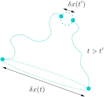
′Fig. 1. Set of trajectories for a pair of fluid parcels evolving ei-ther forwards (t >t′) or backwards (t <t′) in time. Their separa-tion is dominated by an exponential behaviour such that δx(t) ∼ eλF(t −t′)δx(t′), where λ
F is the Lyapunov exponent of the flow.
The dotted lines represent the stretching of a blob of fluid into a filament by the flow.
els used to describe both the flow and the biology are pre-sented. The numerical scheme employed is explained in Sect. 3 along with the tools used to interpret the results. Sec-tion 4 contains the numerical results which illuminate the apparent contradiction between previous results that is the primary focus of this paper. The conclusions are given in Sect. 5.
2 Biological-fluid coupling
In the numerical investigations undertaken, we will assume that the flow v(x, t ) is unsteady, two-dimensional and incom-pressible. These conditions are usually enough to ensure the chaotic advection of fluid parcels, even if the velocity field is a smooth function of space (Ottino, 1989). A way to charac-terise the flow is to look at its Lyapunov exponent, λF,
de-fined as the exponential rate of separation of initially neigh-bouring fluid particles (Fig. 1). Since the fluid is incompress-ible, its volume must be conserved, and therefore contraction must take place in another direction. Moreover, the contrac-tion and also the expansion occur at the same exponential rate
λF. Consequently, blobs of fluid stretch along long and thin
filaments and are repeatedly folded, thus transferring large-scale inhomogeneities into smaller ones.
Although the detailed flow used by Abraham (1998) was different, the essential points characterising the strain dom-inated regions between the eddy regions is captured by the
flow used here. The domain of the velocity field is taken to be a periodic square with side length L, approximately 50 km, corresponding to the characteristic lengthscale of a mesoscale eddy. It will represent the regions that are formed between large eddies, where the phytoplankton filaments are usually observed. This is a pure strain velocity field whose form is v(x, t )= −2 T2(T /2 − t mod T ) cos(2πy/L + φ) −2 T2(t mod T − T /2) cos(2π x/L + θ ) , (1) where 2(t ) is the Heaviside step function defined to be equal to unity for t ≥ 0 and zero otherwise. The phase angles θ and
φ change randomly at each period T of the flow, varying the
directions of expansion and contraction and hence ensuring all parts of it are equally mixed (Bohr et al., 1998; Ott, 1993). Variation of T has an effect on the magnitude of λF without
changing the shape of the trajectories and spatial structure of the flow.
A number of independent fluid parcels are advected by this velocity field. Each one of them carries a uniform distribu-tion of phytoplankton P and zooplankton Z, the latter ap-plied mostly to copepod species, as these can be assumed to be drifting with their respective fluid parcels (Abraham, 1998). On the other hand, large zooplankton, such as krill, actively modify their distributions by swimming (Trathan et al., 1993). Moreover, the model described is intended to only represent larger scales (greater than 100 m or so) on which the flow is quasi two-dimensional. Hence, neglecting any microscopic species motion, e.g. through locomotion or buoyancy, can be justified.
The interactions among the biological species are de-scribed in a model already employed by Abraham (1998). This is a typical nutrient-predator-prey system (Murray, 1993), where the former is parametrised by the carrying ca-pacity. This quantity, denoted as C, is carried along with the fluid parcel and is defined as the maximum phytoplankton content that the parcel can support in the absence of grazing. As the fluid parcel moves through the domain, the carrying capacity continuously relaxes to a space varying background source, C0(x, y)=(1− cos(2π(x+y)/L)), where x and y are
the domain’s horizontal and vertical axes respectively. A large scale inhomogeneity is thus introduced into the system. The species’ dynamics are described by the following di-mensionless equations, dC dt =α(C0(x) − C), (2a) dP dt =P (1 − P /C) − P Z, (2b) dZ dt =P (t − τ )Z(t − τ ) − δZ 2, (2c)
where t is the dimensionless time scaled to the phytoplank-ton production rate r=0.5d−1(t /r is the real time), α denotes the rate at which the carrying capacity relaxes to the back-ground source C0, δ is the zooplankton mortality rate and
τ/r represents the time taken for the zooplankton to mature.
Although it is plausible to assume an instantaneous change in the prey population once prey and predator are encoun-tered, it is not reasonable to assume an instantaneous change in the predator population, and this is the motivation behind the employment of this maturation time.
The phytoplankton growth is logistic and the grazing takes place according to a simple P Z term. In the absence of ad-vection, the parcel position x remains unchanged. In this case, the model has a single fixed point of equilibrium given by C⋆=C0(x), P⋆=δC⋆/(δ+C⋆) and Z⋆=P⋆/δ. This point
is a stable fixed point of equilibrium for τ =0, meaning that any perturbation around this point will eventually decay to zero. If C0≤1 and δ≥0.5, as in the simulations performed
here, it remains stable for any maturation time.
In the presence of advection, this equilibrium point can never be reached due to the continually varying carrying ca-pacity within the fluid parcel. The continual input of large-scale inhomogeneities injected by C0(x) and their transfer to
smaller scales by advection leads to a non-trivial statistical steady state. The study of the induced complex patterns will be the focus of the next sections.
3 Methodology
The planktonic distributions at a particular time are recon-structed by following an ensemble of fluid parcels. In the method used by Abraham (1998), the fluid parcels are tracked forwards in time and the corresponding distributions are obtained from a Delaunay triangulation of the parcel po-sitions by linear interpolation onto a regular grid. Here, the parcels final positions are fixed to a grid. The parcels are then tracked backwards in time up to a time when their ini-tial biological concentration fields are known. Thereafter, knowing their trajectory, their biological evolution is deter-mined by integrating along this trajectory up to the final time using a second order Runge-Kutta method. This way, no in-terpolation is necessary and consequently greater accuracy at smaller length scales is achieved. For the concentrations to be accurate up to three decimal places, the timestep is chosen to be 0.001. This value in real time corresponds to 0.002d and is in line with the assumption made of uniformly dis-tributed populations within the fluid parcels. The ensemble of fluid parcels considered here is 250 000 and evenly spans a grid of resolution 500×500. Their initial concentrations are set to be equal to their mean equilibrium values.
A statistical steady state is reached after 20T , where T is the period of the flow. The emerging patterns are complex in space (Fig. 3). The standard way to characterise such struc-tures is by their Fourier power spectra. Here, we will also
176 A. Tzella and P. H. Haynes: Small-scale spatial structure in plankton distributions 0 0.05 0.1 0.15 0.2 0.25 0.3 0.35 0 0.2 0.4 0.6 0.8 1 α γ α/λF=1 filamental smooth
Fig. 2. Variation of the small-scale structure for the phytoplank-ton carrying capacity in response to the rate α, at which it relaxes towards a smoothly varying background source. The structure is characterised by the H¨older exponent, γ , whose value depends on the ratio of α over the Lyapunov exponent λF. When this ratio is
bigger than 1 the corresponding structure is smooth otherwise it is filamental. The dots mark γ averaged over 500 evenly spaced in-tersections, while the straight line represents its theoretical value. During this set of experiments, λF ∼0.135.
consider their first-order structure function (Monin and Ya-glom, 1975) defined by
S(δx) ≡ h|c(x + δx) − c(x)|i ∼ (δx)γ, (3) where h...i denotes averaging over different values of the co-ordinate x. The scaling exponent, γ , known as the H¨older ex-ponent, is related to the power spectrum exex-ponent, β, by the simple relationship β=1+2γ , where 0<γ <1 corresponds to a rough structure and γ =1 to a smooth one.
4 Numerical results
The emergent spatial structures depend on the relative strength of the dispersion of the parcel trajectories and the stability of the biological dynamics. The phytoplankton car-rying capacity, whose biological evolution is described by Eq. (2a), has a structure that has been shown in Neufeld et al. (1999) to be characterised by two types of behaviour that de-pend on the interplay between the relaxation rate α and the Lyapunov exponent λF. According to the simplest theory
presented in Neufeld et al. (1999), if α>λF, the biological
processes converge faster to their equilibrium value than the trajectories diverge from each other. The corresponding dis-tribution is smooth. On the other hand, if α<λF, the
bio-logical processes are too slow to forget the different spatial histories experienced by the parcels. The corresponding dis-tribution is rough, with a H¨older exponent γ =α/λF in all
di-rections except for the one that the filaments grow into. This type of structure has been defined by Neufeld et al. (1999)
x y 0.2 0.4 0.6 0.8 1 0.2 0.4 0.6 0.8 1 0.1 0.2 0.3 0.4 0.5 0.6 0.7 0.8 0.9
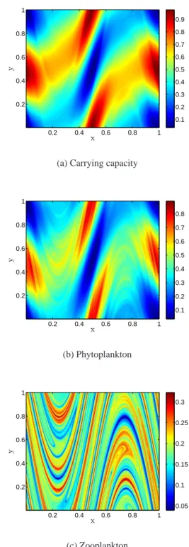
(a) Carrying capacity
x y 0.2 0.4 0.6 0.8 1 0.2 0.4 0.6 0.8 1 0.1 0.2 0.3 0.4 0.5 0.6 0.7 0.8 (b) Phytoplankton x y 0.2 0.4 0.6 0.8 1 0.2 0.4 0.6 0.8 1 0.05 0.1 0.15 0.2 0.25 0.3 (c) Zooplankton
Fig. 3. Snapshots of the biological distributions at statistical equi-librium (t=20T ). The model follows Eq. (2) with τ/r=25d and δ = 2, denoting a high mortality zooplankton regime. The smoothly varying force C0(x, y)=(1−cos(2π(x+y)/L)) is diagonally
orien-tated. The bar on the right gives the concentration values associated with the different colours. The flow is described in equation 1 where the period T =20. The axes are measured in units of L, where L is approximately 50 km.
as filamental. The transition from a filamental to a smooth structure as α varies is depicted in Fig. 2. The numerical agreement with the theoretical prediction gives confidence in the method used here. This is true apart from a small region around α/λF=1. The behaviour in this region is not captured
by the simple theory presented in Neufeld et al. (1999) and is believed to result from the fact that lengthscales are finite and that there is a distribution of finite time Lyapunov exponents. As in Abraham (1998), α is taken to be equal to 0.25 cor-responding to a tracer that takes 8d to adapt to a background force. Choosing a flow with λF∼0.135 (achieved by
set-ting the period to T =20), the emerging phytoplankton carry-ing capacity structure is smooth. This is similar to physical quantities such as the sea surface temperature whose spec-tral slope has been measured to be β=3, equivalent to γ =1 (Deschamps et al., 1981). The limit of α tending to zero cor-responds to a tracer that takes an infinite time to adapt to a background source, i.e. a passive non-reactive tracer. Its ex-pected exponent in a two-dimensional turbulent flow is β=1 or γ =0 (Powell and Okubo, 1994). The above suggests that although the model considered is simple, it is adequate to de-scribe the transfer of variability to smaller scales and hence capture the basic features of turbulence. Moreover, the ex-act details of the flow are not important as long as the fluid parcels are chaotically advected.
For a general biological system, the same smooth filamen-tal transition can be obtained. A system similar to the one described in Eq. (2), in the absence of a maturation time (τ =0), has previously been examined in Hern´andez-Garcia et al. (2002). In this case, the phytoplankton and zooplank-ton populations always share the same small-scale structure. This is not the case for the carrying capacity, due solely to it not being symmetrically coupled to the rest of the popula-tions.
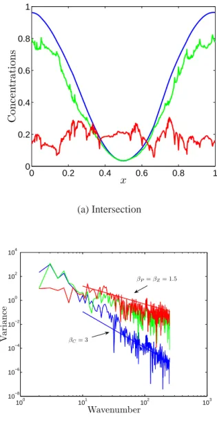
Using the same flow as before, a new set of numerical ex-periments is carried out, with the same biological param-eters used by Abraham (1998). Because of the numeri-cal method used, higher spatial resolution can be achieved. Here, the length scales considered reach 0.002L, (∼100 m, the scale at which turbulence ceases to be two-dimensional). The induced spatial patterns can be seen in Fig. 3. At first sight, the phytoplankton and zooplankton populations seem to be decoupled at all length scales, comfirming the picture given by Abraham (1998). However, a transect through the model domain (Fig. 4) shows that at small enough length scales, both phytoplankton and zooplankton exhibit a fine scale structure. Their corresponding power spectra (Fig. 4) reveal that at large wavelengths (k > 10/L∼0.2 km−1), they share the same structure with a spectral exponent larger than 1. As expected, the carrying capacity behaves smoothly at all scales. At smaller wavelengths, corresponding to larger length scales, the picture provided by Abraham (1998) is re-covered with the phytoplankton spectral slope steepening and the zooplankton one flattening out.
Perhaps a better way to picture this transition is by
look-0 0.2 0.4 0.6 0.8 1 0 0.2 0.4 0.6 0.8 1 x C o n c e n tr a ti o n s (a) Intersection 100 101 102 103 10−8 10−6 10−4 10−2 100 102 104 Wavenumber V a ri a n ce βP= βZ= 1.5 βC= 3 (b) Power Spectrum
Fig. 4. A representative transect (at y=0.5L) and the corre-sponding spectra. Graphs show carrying capacity (blue), phyto-plankton (green) and zoophyto-plankton (red). The spectra are obtained over 500 evenly spaced horizontal transects and have a power law form. The spectral exponents of the populations are βC=3 and
βP=βZ=1.5. The horizontal axes are measured in units of length
L and wavenumber 1/L respectively .
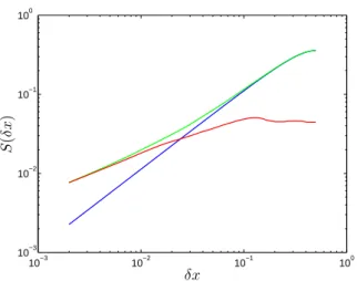
ing at the corresponding first-order structure functions as the length scale δx increases (Fig. 5). Initially, the phytoplankton and zooplankton share similar structures. As δx increases, there is a regime change where the phytoplankton population starts differentiating from the zooplankton population until it completely decouples it at a characteristic lengthscale δxc,
where δxc is approximately equal to 10−1L(∼ 5 km). At
this point the phytoplankton acquires a similar distribution to the carrying capacity, while the zooplankton distribution becomes increasingly flat.
178 A. Tzella and P. H. Haynes: Small-scale spatial structure in plankton distributions 10−3 10−2 10−1 100 10−3 10−2 10−1 100 δx S ( δ x)
Fig. 5. First-order structure functions averaged over 500 evenly spaced horizontal transects. The graph shows carrying capacity (blue), phytoplankton (green) and zooplankton (red). The horizon-tal axes are measured in units of length L. The H¨older exponent of the carrying capacity is γC=1. The phytoplankton and
zoo-plankton respective exponents vary with δx. For δx<δxc, where
δxc≈10−1L, γP=γZ=0.5. For δx>δxc, γC=γP=1 and γZ=0.
5 Conclusions
The small-scale structure of interacting nutrient, phytoplank-ton and zooplankphytoplank-ton populations, passively advected by a two-dimensional flow and coupled to it through an inhomo-geneous source, is here discussed. The particular focus is on the effect induced in these structures by introducing a matu-ration time in the zooplankton growth.
According to Hern´andez-Garcia et al. (2002), given a par-ticular class of flow and in the absence of a maturation time, the small-scale structure for the phytoplankton and zooplank-ton should be the same, given that they are symmetrically coupled, and characterised by a single exponent at all small scales. The inclusion of a maturation time, τ , should not alter the above conclusions. Although the nature of the equa-tions changes from ordinary to delay, there still exists a set of biological decay rates, shared by the phytoplankton and the zooplankton, that should dictate their common structure at small enough scales. This is in disagreement with the nu-merical results obtained in Abraham (1998). There, the phy-toplankton and the carrying capacity turn out to have similar distributions, close to a smooth one and completely decou-pled to the zooplankton’s. As τ increases, the zooplankton’s distribution becomes increasingly filamental, ultimately be-having like a passive tracer (β→1 or γ →0). The aim of this work has been to resolve this disagreement.
Using a model flow to depict the strain dominated regions formed between mesoscale eddies, we reproduce the regime observed by Abraham (1998). However, the alternative nu-merical method used here permits the study of smaller length scales where it is revealed that this is only part of the true
picture: as long as small enough length scales are consid-ered, a second regime appears where the phytoplankton and zooplankton distributions share the same small-scale struc-ture. The transition between these two regimes occurs at a characteristic lengthscale.
It is important to note that although the biological model under consideration is highly simplified, it can be readily ex-tended by including other species or space-dependent pro-ductivity and death rates and these extensions leave the above conclusions unchanged. As long as the biological system remains stable, with a single attractor, the emerging struc-tures will be characterised by a set of spectral exponents or H¨older exponents that will be determined by the competition between the slowest decay rate associated with the biolog-ical processes (though when the biologbiolog-ical model is space-dependent this decay rate will depend to some extend on the flow) and the Lyapunov exponent associated with the stretch-ing properties of the flow.
By introducing a maturation time, both the phytoplankton and zooplankton structures can no longer be characterised by a single exponent at all scales smaller than that of the flow. Perhaps this point, along with the shared exponent at small enough length scales, should be taken into account in try-ing to interpret observational measurements in phytoplank-ton and zooplankphytoplank-ton distributions at a large range of length-scales.
The conditions under which the decoupling of zooplank-ton and phytoplankzooplank-ton take place are still not completely understood. The effect that the biological and the flow activity have on the characteristic length size of the plankton distributions is the subject of current theoretical investiga-tions that will be reported elsewhere. While many issues remain to be resolved, it is hoped that the present paper will provide another step towards understanding the complicated dynamics of plankton in the presence of oceanic fluid motions.
Edited by: E. Boss
References
Abraham, E. R.: The generation of plankton patchiness by turbulent stirring, Nature, 391, 577–580, 1998.
Aref, H.: Stirring by chaotic advection, J. Fluid Mech., 143, 1, 1984.
Bohr, T., Jensen, M., Paladin, G., and Vulpiani, A.: Dynamical Systems Approach to Turbulence, Cambridge University Press, Cambridge, 1998.
Deschamps, P., Frouin, R., and Wald, L.: Satellite determinations of the mesoscale variability of the sea surface temperature, J. Phys. Oceanogr., 11, 864–870, 1981.
Haynes, P. H.: Transport, stirring an mixing in the atmosphere in Mixing – Chaos and turbulence, edited by: Chate, H., Viller-maux, E., and Chomaz, J. M., Kluwer, Dordretch, 1999.
Hern´andez-Garcia, E., L´opez, C., and Neufeld, Z.: Spatial patterns in chemically and biologically reacting flows., Proceedings of the 2001 ISSAOS School on Chaos in Geophysical Flows, Otto editore (Torino 2003), 2001.
Hern´andez-Garcia, E., L´opez, C., and Neufeld, Z.: Small-scale structure of nonlinearly interacting species advected by chaotic flows, CHAOS, 12, 470, 2002.
Kiørboe, T. and Sabatini, M.: 1995 Scaling and fecundity, growth and development in marine planktonic copepods., Mar. Ecol. Prog. Ser., 120, 285–298, 1995.
Klein, P. and Hua, B. L.: The mesoscale variability of the sea sur-face temperature: An analytical and numerical model., Journal of Marine Research, 48, 729–763, 1990.
Martin, A. P.: Phytoplankton patchiness: the role of lateral stirring and mixing, Progress in Oceanography, 57, 125–174, 2003. Martin, A. P. and Srokosz, M. A.: Plankton distribution spectra:
inter-size class variability and the relative slopes for phytoplank-ton and zooplankphytoplank-ton., Geophys. Res. Lett., 29, 2213, 2002. McWilliams, J., Weiss, J., and Yavneh, I.: Anisotropy and coherent
vortex structures in planetary turbulence, Science, 264, 410–413, 1994.
Monin, A. S. and Yaglom, A. M.: Statistical Fluid Mechanics, MIT Press, Cambridge, 1975.
Murray, J. D.: Mathematical Biology, Springer-Verlag, New York, 1993.
Neufeld, Z., L´opez, C., and Haynes, P. H.: Smooth-Filamental Transition of Active Tracer Fields Stirred by Chaotic Advection, Phys. Rev. Let., 82, 2606, 1999.
Okubo, A.: Oceanic diffusion diagrams, Deep-Sea Res., 18, 802, 1971.
Ott, E.: Chaos in Dynamical Systems, Cambridge University Press, Cambridge, 1993.
Ottino, J. M.: The kinematics of mixing: Stretching, chaos and transport., Cambridge University Press, Cambridge, 1989. Powell, T. M. and Okubo, A.: Turbulence diffusion and patchiness
in the sea, Phil. Trans. R. Soc. Lond. B, 343, 11–18, 1994. Seuront, L., Schmitt, F., Lagadeuc, Y., Schertzer, D., Lovejoy, S.,
and Frontier, S.: Multifractal analysis of phytoplankton biomass and temperature in the ocean., Geophys. Res. Lett., 23, 3591– 3594, 1996.
Seuront, L., Schmitt, F., Lagadeuc, Y., Schertzer, D., and Lovejoy, S.: Universal multifractal analysis as a tool to characterize mul-tiscale intermittent patterns: example of phytoplankton distribu-tion in turbulent coastal waters., J. Plankton Res., 21, 977–922, 1999.
Trathan, P. N., Priddle, J., Watkins, J. L., Miller, D. G. M., and Mur-ray, A. W. A.: Spatial variabiity of Antarctic krill in relation to mesoscale hydrography., Mar. Ecol. Prog. Ser., 98, 61–71, 1993. Tsuda, A., Sugisaki, H., Ishimoru, T., Saino, T., and Sato, T.: White-noise-like distribution of the oceanic copepod Neocalanus cristatus in the subarctic North Pacific., Mar. Ecol. Prog. Ser., 97, 39–46, 1993.