The Global Atmospheric Environment for the Next Generation

HAL Id: hal-03048267

https://hal.archives-ouvertes.fr/hal-03048267

HAL is a multi-disciplinary open access

archive for the deposit and dissemination of sci-entific research documents, whether they are pub-lished or not. The documents may come from teaching and research institutions in France or abroad, or from public or private research centers.

L’archive ouverte pluridisciplinaire HAL, est destinée au dépôt et à la diffusion de documents scientifiques de niveau recherche, publiés ou non, émanant des établissements d’enseignement et de recherche français ou étrangers, des laboratoires publics ou privés.

The Global Atmospheric Environment for the Next

Generation

F. Dentener, D. Stevenson, K. Ellingsen, T. van Noije, M. Schultz, M. Amann,

C. Atherton, N. Bell, D. Bergmann, I. Bey, et al.

To cite this version:

F. Dentener, D. Stevenson, K. Ellingsen, T. van Noije, M. Schultz, et al.. The Global Atmospheric Environment for the Next Generation. Environmental Science and Technology, American Chemical Society, 2006, 40 (11), pp.3586-3594. �10.1021/ES0523845�. �hal-03048267�

UCRL-JRNL-217619

The Global Atmospheric

Environment for the Next

Generation

F. Dentener, D. Stevenson, K. Ellingsen, T. van Joije, M. Schultz, M. Amann, C. Atherton, N. Bell, D. Bergmann, I. Bey, L. Bouwman, T. Butler, J. Cofala, B. Collins, J. Drevet, R. Doherty, B. Eickhout, H. Eskes, A. Fiore, M. Gauss, D. Hauglustaine, L. Horowitz, I. S. A. Isaksen, B. Josse, M. Lawrence, M. Krol, J. F. Lamarque, V. Montanaro, J. F. Muller, V. H. Peuch, G. Pitari, J. Pyle, S. Rast, J. Rodriguez, M. Sanderson, N. H. Savage, D. Shindell, S. Strahan, S. Szopa, K. Sudo, R. Van Dingenen, O. Wild, G. Zeng

December 8, 2005

Disclaimer

This document was prepared as an account of work sponsored by an agency of the United States Government. Neither the United States Government nor the University of California nor any of their employees, makes any warranty, express or implied, or assumes any legal liability or responsibility for the accuracy, completeness, or usefulness of any information, apparatus, product, or process

disclosed, or represents that its use would not infringe privately owned rights. Reference herein to any specific commercial product, process, or service by trade name, trademark, manufacturer, or otherwise, does not necessarily constitute or imply its endorsement, recommendation, or favoring by the United States Government or the University of California. The views and opinions of authors expressed herein do not necessarily state or reflect those of the United States Government or the University of California, and shall not be used for advertising or product endorsement purposes.

The global atmospheric environment for the next generation

F.Dentener1, D.Stevenson2, K.Ellingsen3, T.van Noije4, M.Schultz18, M.Amann5, C.Atherton12, N.Bell9, D.Bergmann12, I.Bey8, L.Bouwman6, T.Butler14, J.Cofala5, B.Collins20, J.Drevet8, R.Doherty2, B.Eickhout6, H.Eskes4, A.Fiore16,M.Gauss3, D.Hauglustaine13, L.Horowitz16, I.S.A. Isaksen3, B.Josse15, M.Lawrence14, M.Krol1, J.F.Lamarque17, V.Montanaro21, J.F.Müller11, V.H.Peuch15, G.Pitari21, J.Pyle19,S.Rast18, J.Rodriguez22, M.Sanderson20, N.H.Savage19, D.Shindell9, S.Strahan10, S.Szopa13, K.Sudo7, R.Van Dingenen1,O.Wild7, G.Zeng19.

1. Joint Research Centre, Institute for Environment and Sustainability, Ispra, Italy. 2. University of Edinburgh, School of Geosciences, United Kingdom.

3. University of Oslo, Department of Geosciences, Norway.

4. Royal Netherlands Meteorological Institute (KNMI), De Bilt, the Netherlands. 5. IIASA, International Institute for Applied Systems Analysis, Laxenburg, Austria. 6. Netherlands Environmental Assessment Agency (RIVM/MNP), Bilthoven, The Netherlands.

7. Frontier Research Center for Global Change, JAMSTEC, Yokohama, Japan. 8. Swiss Federal Institute of Technology (EPFL), Lausanne, Switzerland. 9. NASA-Goddard Institute for Space Studies, New York, USA.

10. Goddard Earth Science & Technology Center (GEST), Maryland, USA. 11. Belgian Institute for Space Aeronomy, Brussels, Belgium.

12. Lawrence Livermore National Laboratory, Atmospheric Science Division, Livermore, USA.

13. CEA/CNRS, Laboratoire des Sciences du Climat et de l'Environnement, Gif-sur-Yvette, France.

14. Max Planck Institute for Chemistry, Mainz, Germany. 15. Meteo-France, CNRM/GMGEC/CATS, Toulouse, France. 16. NOAA GFDL, Princeton, NJ, USA.

17. National Center of Atmospheric Research, Atmospheric Chemistry Division, Boulder, CO, USA.

18. Max Planck Institute for Meteorology, Hamburg, Germany.

19. University of Cambridge, Centre of Atmospheric Science, United Kingdom. 20. Met Office, Exeter, United Kingdom.

21. Università L'Aquila, Dipartimento di Fisica, Italy.

22. University of Miami/NASA-Goddard Space Flight Center Submitted ES&T, 01.12.2005

Abstract

Air quality, ecosystem exposure to nitrogen deposition, and climate change are intimately coupled problems: we assess changes in the global atmospheric environment between 2000 and 2030 using twenty-five state-of-the-art global atmospheric chemistry models and three different emissions scenarios. The first (CLE) scenario reflects implementation of current air quality legislation around the world, whilst the second (MFR) represents a

more optimistic case in which all currently feasible technologies are applied to achieve maximum emission reductions. We contrast these scenarios with the more pessimistic IPCC SRES A2 scenario. Ensemble simulations for the year 2000 are consistent among models, and show a reasonable agreement with surface ozone, wet deposition and NO2

satellite observations. Large parts of the world are currently exposed to high ozone concentrations, and high depositions of nitrogen to ecosystems. By 2030, global surface ozone is calculated to increase globally by 1.5±1.2 ppbv (CLE), and 4.3±2.2 ppbv (A2). Only the progressive MFR scenario will reduce ozone by -2.3±1.1 ppbv. The CLE and A2 scenarios project further increases in nitrogen critical loads, with particularly large impacts in Asia where nitrogen emissions and deposition are forecast to increase by a factor of 1.4 (CLE) to 2 (A2). Climate change may modify surface ozone by -0.8±0.6 ppbv, with larger decreases over sea than over land. This study shows the importance of enforcing current worldwide air quality legislation, and the major benefits of going further. Non-attainment of these air quality policy objectives, such as expressed by the SRES-A2 scenario, would further degrade the global atmospheric environment.

Introduction

Emissions of reactive nitrogen, i.e. nitrogen oxides (NOx = NO + NO2), generated in the

burning of fossil- and bio-fuels, and ammonia (NH3) volatilized from agricultural

processes, cause a number of environmental problems. Ozone (O3) is formed in the

presence of NOx, methane (CH4), carbon monoxide (CO) and hydrocarbons. O3 is an

important greenhouse gas and is also toxic to humans, animals and plants. The IPCC Third Assessment Report (1) recognized the intertwined role of CH4 and conventional air

pollutant emissions for climate and air quality. In particular, an evaluation of the high-emissions IPCC SRES A2 high-emissions scenario showed global mean surface O3 increases

of about 5 ppbv by 2030 and 20 ppbv by 2100 (2). Another associated adverse impact of the enhanced emissions of NOx and NH3 is the increased long-range transport and

deposition of nitrogen, leading to damaging eutrophication and acidification of ecosystems and loss of biodiversity (3,4).

In this work we focus on climate change, air quality, and ecosystem exposure to nitrogen deposition for the year 2030. We use a new set of emission scenarios for CH4, NOx, NH3,

CO, SO2 and non-methane volatile organic compounds (NMVOC) recently developed at

IIASA (International Institute for Applied Systems Analysis) and described by (5). The scenarios differ substantially from the previous SRES (6) scenarios. In the last few years increasing air pollution in developing countries has become a public concern (5, and references therein). As a consequence many of the major rapidly developing countries in Asia and Latin America have issued legislation on state-of-the-art emission controls. Upon implementation, these regulations will significantly cap the air pollution emissions at the regional and global scales. This is the basis of our CLE (Current LEgislation) scenario. Further, we evaluate the effects of the emissions of a MFR (Maximum

technologically Feasible Reduction) scenario, and contrast it with the pessimistic SRES A2 scenario. Both CLE and MFR are based on economic and energy use projections according to the moderate SRES B2 scenario. These emission scenarios were used by 25

global atmospheric chemistry-transport models (CTMs) driven by re-analyzed

meteorological fields or general circulation models (GCMs), run by groups in Europe, the United States, and Japan. Although some models share some common sub-components, the ensemble of model results is sufficiently broad to estimate uncertainties resulting from the various assumptions in the transport models. The models performed baseline (year 2000) and 2030 scenarios, all using a fixed meteorology based on the year 2000; whereas a subset of models repeated the 2030 CLE scenario, but with a changed climate. In this paper we give an integrative overview of the findings; other publications (7-10) present more detailed results from this large model exercise.

Methods

Up to five simulations were performed by each model (Table 1). B2000 evaluated the reference year 2000, whilst CLE, MFR, and A2 assessed the year 2030. CTMs used the meteorological year 2000. GCMs performed 5-10 years of simulations, using a climate appropriate for the time period 1995-2004. To evaluate the impacts of climate change, an additional simulation (CLE2030c) was computed by nine of the GCM-driven models, using a climate appropriate for 2030. Most modelers applied the IS92a climate scenario associated with a global mean surface warming of about 0.7K between 2000 and 2030. Global emissions of NOx, CO, NMVOC, and CH4 (Table 1) were generated by IIASA,

and spatially distributed using the EDGAR3.2 database, as described in and references therein. NH3 emissions were generated by RIVM IMAGE model

(http://arch.rivm.nl/image ). To avoid excessive spin-up times for equilibration of CH4 we

prescribed global CH4 volume mixing ratios instead of emissions [Table 1], using

consistent values from earlier transient simulations for 1990-2030 described in (5,11). In electronic supplement Table ES1 we present the 25 participating models, including characteristics of their resolution, chemistry and transport parameterizations. Compared to the earlier modeling exercises (2,12) twice as many models participated in this study; model complexity (inclusion of NMVOC chemistry), and resolutions have greatly improved: almost half of the models had horizontal resolutions of 2º-3º or better, and almost of the other models had resolutions around 4º-5º. Further information on the model experiment can be found on http://www2.nilu.no/farcry_accent.

Results

Surface ozone increases

In Figure 1a-1d we display the annual average O3 and O3 differences at the earth surface

calculated from all models for B2000, CLE,MFR, and A2 in 2030. The impact of climate change (CLE2030c) is given in Figure 1e. Figure 1a shows that calculated annual average surface O3 varies between 40-50 ppbv over large parts of N. America, S. Europe, and

Asia. Background values ranging between 15-25 ppbv are found in large parts of the S. Hemisphere (SH). Average surface concentrations are 33.7 ± 3.8, 23.7 ± 3.7 and 28.7 ± 3.6 ppbv (Table 2), for the N. Hemisphere (NH), SH, and world, respectively. In Figure 1a we also give averaged measurements for the year 2000, taken from the WMO-GAW World Data Centre for surface ozone, EMEP/AIRBASE in Europe; and CASTNet in the

United States. Measurements for India, China, and Africa are from various scientific studies (13-16). Our analysis reveals that our mean model results agree within 5 ppbv with measurements in the USA, China, and Central Europe, and may overestimate the measured annual average with 10-15 ppbv in Africa, India and the Mediterranean. The variability among the annual model results was of the order 10-30 %.

The CLE scenario (Figure 1b, Table 2) would approximately stabilize O3 in 2030 at 2000

levels in parts of N. America, Europe and Asia. However, O3 may increase by more than

10 ppbv in areas anticipated to experience large increases of transport and power generation related emissions (e.g. India). Background O3 increases by 2-4 ppbv in the

tropical and mid-latitude NH, related to the interaction of the increasing concentrations of CH4 and the worldwide increase of emissions of NOx, CO, and NMVOC. The increases

are most consistently predicted in Asia; whereas the ensemble predictions are not robust (large standard deviations) in North and South America, Southern Africa and the Middle East. A cleaner future is possible, if all currently available technologies are used to abate O3 precursor emissions. In this MFR case (Figure 1c; Table 2) O3 reduces by 5-10 ppbv

relative to the present situation in the regions of main pollution. The models are consistent in their prediction of the ozone reductions with relative standard deviations around 30-40%. Finally, consistent with previous studies (2), in the A2 scenario (Figure 1d), annual average surface O3 increases by 4.3 ppbv worldwide and by 5-15 ppbv in

Latin America, Africa and Asia.

How is climate change expected to influence these O3 changes? The average results from

9 models for the CLE2030c scenario indicate that climate change may reduce surface O3

by 1-2 ppbv over the oceans, and by 0.5 to 1 ppbv over the continents. We find that the climate change related processes affecting surface O3 were the regional and global

increase of temperature and water vapor, tending to decrease surface O3, particularly in

the cleanest regions, and the increased influx of stratospheric O3 into the troposphere,

increasing free tropospheric and surface O3. Note that many feedbacks, e.g. from natural

emission changes, were generally not included in the models. We further note that the variability in the calculated climate induced ozone perturbations is large [Table 2], associated with the differences of individual climate model simulations.

What is the effect on ozone air quality? Several regulatory O3 air quality limits, with

threshold values of 60-80 ppbv, are currently employed in Europe, the USA and Japan. The World Health Organization (WHO) re-analyzed epidemiological studies of O3

related health effects, and recommend the air quality index called SOMO35

(http://www.unece.org/env/documents/2004/eb/wg1/eb.air.wg1.2004.11.e.pdf). SOMO35 is based on the exceedance over 35 ppbv “background level” of the daily maximum of an 8-hour running average ozone volume mixing ratio (MaxO3):

[

]

∑

In contrast to other air quality limits, SOMO35 considers O3 toxicity at lower

concentrations; and is more suited to assess the effect of large scale changes of ozone background concentrations. Figure 2 gives the SOMO35 for scenario S1-S4, and in Table 2 we give a regional analysis of SOMO35. Ellingsen et al. (8) show that a SOMO35 of ~ 3000 ppb days is consistent with air quality limits currently in use in North America and Europe. According to our model calculations SOMO35 is exceeded in large parts of the world in the year 2000; most notably in the United States, the Middle East, and South Asia (India). In these regions most models consistently compute SOMO35 in excess of 3000 ppb.days. Only in the MFR scenario ozone will be close to the WMO airquality limit. The large scale regional and annual averaged ozone and SOMO35 appear to be highly correlated with a correlation coefficient of r=0.99; this high correlation follows from the fact that already at present background ozone is close to the 35 ppbv threshold.

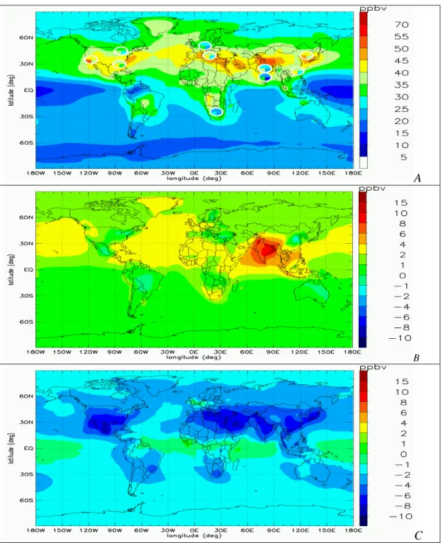
Nitrogen deposition

In Figure 3a-d we give the calculated NOy total deposition averaged for 22 models in

2000, CLE, MFR, and A2 2030. Figure 3e gives the total reactive nitrogen (=NOy+NHx)

deposition in the year 2000, showing the importance of NHx deposition. It is currently thought that 1000 mgNm-2yr-1 is a threshold (“critical load”), above which changes in sensitive natural ecosystems may occur (4,17). So far most studies have focused on the effects of NOy deposition (18), since it is intimately associated with O3 formation. Our

results indicate that accounting for NHx deposition, related to animal and food production

systems, may double the deposition from NOy alone. The resulting total Nitrogen (NOy

and NHx) deposition exceeds 2000 mgNm-2yr-1 in extended parts of the world, including

biodiversity hotspots. To date, the consequences for biodiversity and ecosystem health have only been studied for temperate regions, but it has been suggested that increased nitrogen deposition will play an important future role in the decrease of plant diversity worldwide (19). A comparison of the corresponding calculated wet deposition fluxes with measurements in USA, Europe, S.E. Asia , Africa and S. America, yields agreement within a factor of two for 70-80 % of the measurement stations (see EF). Exceptions are Asia where the models strongly underestimate NOy deposition by up to 60 %, and S.

America, where almost no measurement data were found. In 2030, considering the CLE scenario NOy deposition decreases in Europe, is near-constant in N. America, and

strongly increases in Asia. NHx depositions increase almost everywhere. Our clean MFR

scenario, which was evaluated only for NOy, considerably improves this situation, with

NOy deposition almost everywhere below 500 mgNm-2yr-1. In contrast, the A2 scenario in

the year 2030 leads to extended regions exposed to NOy deposition larger than 1000

mgNm-2yr-1.

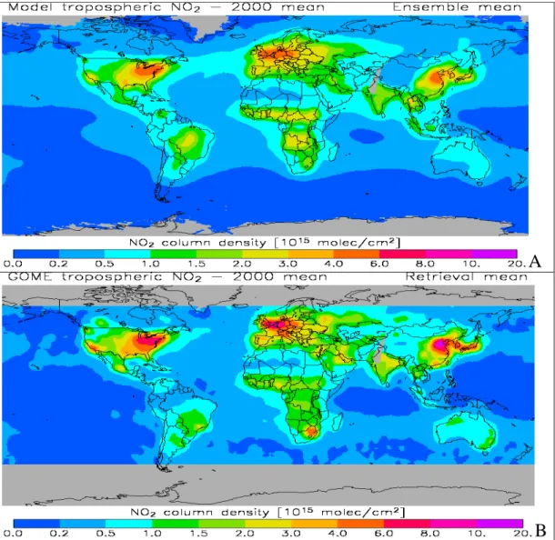
Satellite observations of NO2 columns

Recent satellite observations allow us to evaluate nitrogen pollution on near global scales. For the year 2000, the GOME instrument on-board of the ERS-2 satellite, provides a unique opportunity to compare model calculated NO2 columns with measurements. We

compare model NO2 column output at the satellite overpass time (10:30 LT), taking into

densities were calculated by 17 different models; uncertainties in the retrievals are quantified by using retrieval products from three different groups: KNMI/BIRA-IASB (20), University of Bremen (21), and an update of the Dalhousie/SAO retrieval (22), excluding uncertain retrievals at high latitudes. Low tropospheric NO2 columns of <1

1015 moleccm-2 are calculated and observed by GOME in marine regions. Over the continents, three regions of dominant NO2 pollution are found in N. America, W.Europe,

and China, coinciding with the regions of high emissions. These regions are also indicated in the average model; but the averaged model maxima of 6-8 1015 moleccm-2 clearly underestimate the GOME observed values, which exceed 10 1015 moleccm-2. The difference of models and measurements is particularly pronounced over the rapidly developing parts of Eastern China and South Africa, indicating that the assumed NOx

emissions may be unrealistically low in these regions. In regions dominated by biomass burning, such as in Africa and South America, the models tend to overestimate the observed seasonal cycle.

We note that the discrepancy in NO2 column in e.g. North America and Europe does not

seem consistent with the general agreement in NO3 wet deposition. In the rapidly

developing parts of China and Southern Africa, the model-satellite discrepancy indicates an underestimate of NO emissions, consistent with underestimates of N-deposition, but not corroborated by similar discrepancies in surface ozone. One important finding, however, is that the differences of the GOME retrievals are in many instances as large as the spread in model results, meaning that in only a few cases(i.e. in China) robust

statements on under prediction of NO emissions can be made.

The present and future atmospheric environment

The results from 25 state-of-the-art atmospheric chemistry transport and climate models regarding changes in surface O3, and deposition of nitrogen are for the year 2000 broadly

consistent with measurements of current day O3, NO2 columns, and nitrogen deposition,

with largest discrepancies in the developing regions of India, Africa, and S.E. Asia. Most models indicate that already in the year 2000, the most recent WHO recommended air quality standard SOMO35 is exceeded over large regions. We considered 3 scenarios for 2030. In the CLE scenario this situation is aggravated in parts of Asia (most notably in India with large growth in the transport sector), whereas the MFR scenario provides a cleaner alternative for O3. Our model results indicate that the undesirable SRES A2

scenario would lead to large problems in 2030 with attaining any air quality standard in most industrialized parts of the world. We also show that NOy and NHx deposition are

already at present above the critical nitrogen loads, resulting in eutrophication and decrease of biodiversity. These deposition fluxes are expected to increase further considering the CLE and A2 scenarios. The same emissions that worsen air quality and nitrogen deposition also have a substantial impact on climate. Stevenson et al. (10) show that the sum of the O3 and CH4 radiative forcings, in case of CLE and A2, contributes

22% - 28% to the forcings of CO2 alone. Only introduction of stringent NOx, CO,

NMVOC, and CH4 abatement technologies (MFR) prevents further increases in the

reducing NOx, CO, NMVOC, and CH4 emissions (5,23,24) is needed to guarantee a

cleaner atmospheric environment for the next generation.

Acknowledgements

This model exercise was organized under the umbrella of the EC FP6 Network of Excellence ACCENT.

This work was performed under the auspices of the U.S. Department of Energy by University of California, Lawrence Livermore National Laboratory under contract W-7405-Eng-48.

References

(1) Prather, M.; Ehhalt, D.; Dentener, F.; Derwent, R.; Dlugokencky, E.; Holland, E.; Isaksen, I.; Katima, J.; Kirchhoff, V.; Matson, P.; Midgley, P.; Wang, M. In Climate

Change 2001, The scientific basis: Contribution of working group I to the Third

assessment report of the Intergovernmental Panel on Climate; Houghton, J. T., Ding, Y.,

Griggs, D. J., Noguer, M., Linden, P. J. v. d., Dai, X., Maskell, K., Johnson, C. A., Eds.; Cambridge University Press: Cambridge, United Kingdom and New York, NY, US, 2001; p 881

(2) Prather, M.; Gauss, M.; Berntsen, T. K.; Isaksen, I.; Sundet, J.; Bey, I.; Brasseur, G.; Dentener, F.; Derwent, R.; Stevenson, D. S.; Grenfell, L.; Hauglustaine, D.;

Horowitz, L. W.; Jacob, D.; Mickley, L. J.; Lawrence, M. G.; Kuhlman, R. v.; Muller, J.-F.; Pitari, G.; Rogers, H.; Johnson, M.; Pyle, J. A.; Law, K. S.; Weele, M. v.; Wild, O. Fresh air in the 21st century. Geophys. Res. Lett 2003, 30, 72-72-74.

(3) Stevens, C. J.; N.B. Dise; J.O. Mountford; Gowing, D. J. Impacts of nitrogen deposition on species richness of grassland. Science 2004, 303, 1876-1879.

(4) Galloway, J. M.; F.J. Dentener; D.G. Capone; E.W. Boyer; R.W. Howarth; S.P. Seitzinger; G.P. Asner; C. Cleveland; P. Green; E. Holland; D.M. Karl; A.F. Michaels; J.H. Porter; A. Townsend; Charles, V. Nitrogen Cycles: Past, Present and Future.

Biogeochemistry 2004, 70, 153-226.

(5) Dentener, F.; D. Stevenson; J. Cofala; R. Mechler; M. Amann; P. Bergamaschi; F. Raes; Derwent, R. The impact of air pollutant and methane emission controls on

tropospheric ozone and radiative forcing: CTM calculations for the period 1990-2030.

Atmospheric Chemistry and Physics 2005, 5, 1731-1755,

SREF-ID:1680-7324/ap/2005-1735-1731.

(6) Nakicenovic, N.; Alcamo, J.; Davis, G.; De Vries, B.; Fenhann, J.; Gaffin, S.; Gregory, K.; Grübler, A.; Jung, T. Y.; Kram, T.; Lebre La Rovere, E.; Michaelis, L.; Mori, S.; Morita, T.; Pepper, W.; Pitcher, H.; Price, L.; Riahi, K.; Roehrl, A.; Rogner, H. H.; Sankovski, A.; Schlesinger, M.; Priyadarshi Shukla, P.; Steven Smith, S.; Robert Swart, R.; Van Rooijen, S.; Victor, N.; Dadi, Z.; Cambridge University press: Cambridge, United Kingdom and New York, USA, 2000; p 599 p.

(7) Dentener, F.; etal. Nitrogen and Sulphur Deposition on regional and global scales: a multi-model evaluation. Global Biogeochemical Cycles 2005, in preparation.

(8) Ellingsen, K.; etal Ozone air quality in 2030: a multi model assessment of risks for health and vegetation. Journal of Geophysical Research 2005, in preparation. (9) van Noije, T.; etal Multi-model ensemble simulations of tropospheric NO2 compared with GOME retrievals for the year 2000. Journal Geophysical Research 2005, in preparation.

(10) Stevenson, D. S.; Dentener, F. J.; Schultz, M. G.; Ellingsen, K.; Van Noije, T. P. C.; Wild, O.; Zeng, G.; M. Amann; Atherton, C. S.; Bell, N.; Bergmann, D. J.; Bey, I.; Butler, T.; Cofala, J.; Collins, W. J.; Derwent, R. G.; Doherty, R. M.; Drevet, J.; Eskes, H. J.; Fiore, A.; Gauss, M. A.; Hauglustaine, D. A.; Horowitz, L. W.; Isaksen, I. S. A.; Krol, M. C.; Lamarque, J. F.; Lawrence, M. G.; Montanero, V.; Müller, J. F.; Pitari, G.; Prather, M. J.; Pyle, J. A.; Rast, S.; Rodriguez, J. M.; Sanderson, M. G.; Savage, N. H.; Shindell, D. T.; Strahan, S. E.; Sudo, K.; Szopa, S. Multi-model ensemble simulations of

present-day and near-future tropospheric ozone. Journal Geophysical Research 2005, accepted.

(11) Stevenson, D.; R. Doherty; M. Sanderson; C. Johnson; B. Collins; Derwent, D. Impacts of climate change and variability on tropospheric ozone and its precursors.

Faraday Discuss 2005, 130, 1-17.

(12) Gauss, M., G. Myhre, G. Pitari, M. J. Prather, I. S. A. Isaksen, T. K. Berntsen, G. P. Brasseur, F. J. Dentener, R. G. Derwent, ; D. A. Hauglustaine, L. W. H., D. J. Jacob, M. Johnson, K. S. Law, L. J. Mickley, J.-F. Müller, P.-H. Plantevin, J. A. Pyle, H. L. Rogers, D. S. Stevenson, J. K. Sundet, M. van Weele, ; Wild, O. Radiative forcing in the 21st century due to ozone changes in the troposphere and the lower stratosphere.

J.Geophys. Res. 2003, 108 (D9), 4292, doi:4210.1029/2002JD002624.

(13) Zunckel, M.; K. Venjonoka; J.J. Pienaar; E.G. Brunke; O. Pretorius; A.

Koosialee; A. Raghunandan; Tienhoven, A. M. v. Surface ozone over southern Africa, synthesis of monitoring results during the cross border Air Pollution Impact Assessment project. Atmos Environ. 2004, 38, 6139-6147.

(14) Carmichael, G. R.; Ferm, M.; Thongboonchoo, N.; Woo, J.-H.; Chan, L. Y.; Murano, K.; Viet, P. H.; Mossberg, C.; Bala, R.; Boonjawat, J.; Upatum, P.; Mohan, M.; Adhikary, S. P.; Shrestha, A. B.; Pienaar, J. J.; Brunke, E. B.; Chen, T.; Jie, T.; Guoan, D.; Peng, L. C.; Dhiharto, S.; Harjanto, H.; Jose, A. M.; Kimani, W.; Kirouane, A.; Lacaux, J.; Richard, S.; Barturen, O.; Cerda, J. C.; Athayde, A.; Tavares, T.; Cotrina, J. S.; Bilici, E. Measurements of sulfur dioxide, ozone and ammonia concentrations in Asia, Africa, and South America using passive samplers. Atm. Env. 2003, 37, 1293-1308. (15) Naja, M.; Lal, S. Surface ozone and precursor gases at Gadanki (13.5 N, 79.2 E) a tropical rural site in India. Journal Geophysical Research 2002, 107, 4179, DOI:

4110.1029/2001JD000357.

(16) Naja, M.; S. Lal; Chand, D. Diurnal and seasonal variabilities in surface ozone at a high altitude site Mt Abu (24.6 N, 72,7 E, 160 ma asl) in India. Atm. Env. 2003, 37, 4205-4215.

(17) Bobbink, R.; M. Hornung; J.M. Roelofs The effects of air-borne pollutants on species diversity in natural and semi-natural European vegetation. Journal of Ecology

1998, 86, 717-738.

(18) Holland, E. A.; B.H. Brasswell; J.F. Lamarque; A. Townsend; J. Sulzman; J.F.Muller; F. Dentener; G.Brasseur; H. Levy II; J.E. Penner; Roelofs, G. J. Variations in the predicted spatial distribution of atmospheric nitrogen deposition and their impact on carbon uptake by terrestial ecosystems. J. Geophys. Res. 1997, 102, 15849-15866. (19) Sala, O. E., F.S. Chapin III, J.J. Armesto, R. Berlow, J. Bloomfield, R. Dirzo, E. Huber-Sanwald, L.F. Huenneke, R.B. Jackson, A. Kinzig, R. Leemans, D. Lodge, H.A. Mooney, M. Oesterheld, N.L. Poff, M.T. Sykes, B.H. Walker, M. Walker, and D.H. Wall, Global biodiversity scenarios for the year 2100. Science 2000, 87, 1770-1774.

(20) Boersma, K. F.; H.J. Eskes; Brinksma, E. J. Error analysis for tropospheric NO2 retrieval from space. J. Geophys. Res. 2004, 109,, doi:10.1029/2003JD003962.

(21) Richter, A.; Burrows, J. P. Retrieval of tropospheric NO2 from GOME measurements. Adv. Space Res. 2002, 29, 1673-1683.

(22) Martin, R. V.; K. Chance; D.J. Jacob; T.P. Kurosu; R.J.D. Spurr; E. Bucsela; J.F. Gleason; P.I. Palmer; I. Bey; A.M. Fiore; Q. Li; R.M. Yantosca; Koelemeijer, R. B. A.

An improved retrieval of tropospheric nitrogen dioxide from GOME. J. Geophys. Res.

2002, 107, 4437, 4410.1029/2001JD001027.

(23) Fiore, A. M.; Jacob, D. J.; Field, B. D.; D. G. Streets; S. D. Fernandes; Jang, C. Linking ozone pollution and climate change: The case for controlling methane. Geophys.

Res. Lett 2002, 29, 25-21/25-24, doi:10.1029/2002GL015601.

(24) West, J. J.; Fiore, A. M. Management of Tropospheric Ozone by Reducing Methane Emissions. Environ. Sci. Technol. 2005, E39(13), 4685-4691,

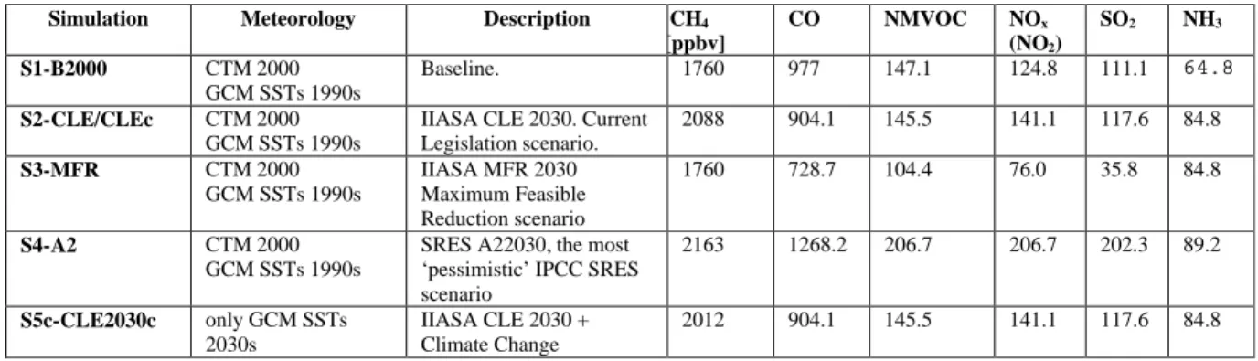
Table 1. Overview of simulations, prescribed methane volume mixing ratios and global anthropogenic emissions of CO, NMVOC, SO2 and NH3. Emissions in Tg Full

Molecular Weight /year.

Simulation Meteorology Description CH4

[ [ppbv] CO NMVOC NOx (NO2) SO2 NH3 S1-B2000 CTM 2000 GCM SSTs 1990s Baseline. 1760 977 147.1 124.8 111.1 64.8 S2-CLE/CLEc CTM 2000 GCM SSTs 1990s

IIASA CLE 2030. Current Legislation scenario. 2088 904.1 145.5 141.1 117.6 84.8 S3-MFR CTM 2000 GCM SSTs 1990s IIASA MFR 2030 Maximum Feasible Reduction scenario 1760 728.7 104.4 76.0 35.8 84.8 S4-A2 CTM 2000 GCM SSTs 1990s

SRES A22030, the most ‘pessimistic’ IPCC SRES scenario 2163 1268.2 206.7 206.7 202.3 89.2 S5c-CLE2030c only GCM SSTs 2030s IIASA CLE 2030 + Climate Change 2012 904.1 145.5 141.1 117.6 84.8

Table 2: Area weighted regional and global annual mean surface ozone [ppbv] and in Italics SOMO35 [ppbv days] in 2000 and increases for various scenarios at selected regions. Regions are defined according to IMAGE2.2

(http://arch.rivm.nl/image/). Standard deviations are calculated from ‘n’ models. The WHO recommended SOMO35 is based on the exceedance of 35 ppbv of the daily maximum of an 8-hour running average ozone volume mixing ratio.

Region O3 2000 n=24/17 ?O3 CLE2030-B2000 n=22/14 ?O3 MFR2030 -B2000 n=19/14 ?O3 A2_2030-B2000 n=18/14 ?O3 CLE2030c -CLE2030 n=9 USA 38.7 ±4.9 4145±1378 1.3±2.4 583±280 -4.9±1.8 -1788±525 4.8± 4.5 1911±797 -0.4±1.2 South America 27.9 ±4.7 1681±865 0.5±2.0 140±74 -2.4±2.3 -231±106 5.7± 2.7 1247 ±597 -0.5±0.8 Southern Africa 34.8 ±5.0 3207±1304 1.4±3.9 553±190 -2.5±4.5 -332±126 7.0± 4.2 2084±666 -0.4±0.7 OECD Europe 36.6 ±4.2 3056±1084 1.8±1.5 384±335 -2.8±1.1 -1071±292 3.9± 3.8 1417 ±823 -0.4±0.7 Middle East _{43.5 ±6.4} 5388±1917 1.7±2.4 766±401 -6.6±2.2 -2195±668 8.7± 6.0 3692±1523 -0.6±0.9 South Asia 45.0 ±6.9 6093±2266 7.2±1.9 3094±791 -5.9±1.6 -1976±560 11.8± 4.3 4914±1435 -0.7±0.9 South East Asia 31.5 ±4.4 2096±937 3.8±0.7 945±329 -3.6±0.5 -703±276 7.7± 1.8 2222±563 -0.6±1.0 Northern Hemisphere 33.7 ±3.8 2336±950 2.3±0.5 615±254 -2.9±0.6 -786±208 5.9±2.1 1738±704 -0.8±0.7 Southern Hemisphere 23.7 ±3.7 486±330 0.6±2.1 111±85 -1.7±2.3 -79±55 2.7± 2.6 394±229 -0.7±0.6 World _{28.7 ±3.6} 1411±608 1.5±1.23 63±160 -2.3±1.1 -433±118 4.3± 2.2 1066±426 -0.8±0.6

Figure 1: (a) Ozone in the year 2000; and the ozone differences between scenarios (b) CLE, (c) MFR, (d) A2 with 2000 and (e) the impact of climate change comparing CLEc and CLE. Differences are based on the averaged difference of individual model simulation. Regionally averaged measurements (upper: mean, lower left mean+1 s , lower right mean-1 s ) are given in the circles.

A

B

D

Figure 2: SOMO35 [ppbv days] (a) in the year 2000; (b) 2030 CLE; (c) 2030 MFR and (d) A2. SOMO35 is based on the daily maximum of an 8 hours moving average ozone volume mixing ratio subtracted by 35 ppbv.

A

C

Figure 3: NOy total deposition averaged for 22 models [mgNm-2 yr-1] in (a) 2000 (b)

CLE 2030 (c), MFR 2030 (d) A2 2030 ; and (e) total reactive nitrogen (=NOy+NHx)

deposition [mgNm-2 yr-1] in 2000.

A

B

D

Figure 4: (a) Modelled and (b) GOME measured annual average NO2 columns for

the year 2000. Modelled data represents an average of 17 models, and the GOME retrieval is an average of three retrieval products. For a consistent comparison, the data in both cases have been smoothed to a horizontal resolution of 5ox5o.

A