HAL Id: hal-00295307
https://hal.archives-ouvertes.fr/hal-00295307
Submitted on 1 Aug 2003
HAL is a multi-disciplinary open access
archive for the deposit and dissemination of
sci-entific research documents, whether they are
pub-lished or not. The documents may come from
teaching and research institutions in France or
abroad, or from public or private research centers.
L’archive ouverte pluridisciplinaire HAL, est
destinée au dépôt et à la diffusion de documents
scientifiques de niveau recherche, publiés ou non,
émanant des établissements d’enseignement et de
recherche français ou étrangers, des laboratoires
publics ou privés.
Svalbard, 78°N
J. Höffner, C. Fricke-Begemann, F.-J. Lübken
To cite this version:
J. Höffner, C. Fricke-Begemann, F.-J. Lübken. First observations of noctilucent clouds by lidar at
Sval-bard, 78°N. Atmospheric Chemistry and Physics, European Geosciences Union, 2003, 3 (4),
pp.1101-1111. �hal-00295307�
www.atmos-chem-phys.org/acp/3/1101/
Chemistry
and Physics
First observations of noctilucent clouds by lidar at Svalbard, 78
◦
N
J. H¨offner, C. Fricke-Begemann, and F.-J. L ¨ubken
Leibniz-Institut f¨ur Atmosph¨arenphysik, K¨uhlungsborn, Germany
Received: 23 October 2002 – Published in Atmos. Chem. Phys. Discuss.: 4 February 2003 Revised: 29 April 2003 – Accepted: 5 June 2003 – Published: 1 August 2003
Abstract. In summer 2001 a potassium lidar was installed
near Longyearbyen (78◦N) on the north polar island of
Spits-bergen which is part of the archipelago Svalbard. At the same place a series of meteorological rockets (“falling spheres”, FS) were launched which gave temperatures from the lower thermosphere to the stratosphere. The potassium lidar is ca-pable of detecting noctilucent clouds (NLCs) and of mea-suring temperatures in the lower thermosphere, both un-der daylight conditions. In this paper we give an overview on the NLC measurements (the first at this latitude) and compare the results with temperatures from meteorological rockets which have been published recently (L¨ubken and M¨ullemann, 2003). NLCs were observed from 12 June (the first day of operation) until 12 August when a period of bad weather started. When the lidar was switched on again on 26 August, no NLC was observed. The mean occurrence frequency in the period 12 June – 12 August (“lidar NLC pe-riod”) is 77%. The mean of all individual NLC peak altitudes is 83.6 km (variability: 1.1 km). The mean peak NLC alti-tude does not show a significant variation with season. The average top and bottom altitude of the NLC layer is 85.1 and 82.5 km, respectively, with a variability of ∼1.2 km. The mean of the maximum volume backscatter coefficient βmax at our wavelength of 770 nm is 3.9×10⁻¹⁰/m/sr with a large variability of ±3.8×10⁻¹⁰/m/sr. Comparison of NLC char-acteristics with measurements at ALOMAR (69◦N) shows that the peak altitude and the maximum volume backscatter coefficient are similar at both locations but NLCs occur more frequently at higher latitudes.
Simultaneous temperature and NLC measurements are available for 3 flights and show that the NLC layer occurs in the lower part of the height range with super-saturation. The NLC peak occurs over a large range of degree of satura-tion (S) whereas most models predict the peak at S = 1. This demonstrates that steady-state considerations may not be
ap-Correspondence to: F.-J. L¨ubken ([email protected])
plicable when relating individual NLC properties to back-ground conditions. On the other hand, the mean variation of the NLC appearance with height and season is in agreement with the climatological variation of super-saturation derived from the FS temperature measurements.
1 Introduction
Noctilucent clouds (NLCs) have been observed since more than 100 years in the upper summer mesosphere at polar and midlatitudes (Leslie, 1885; Gadsden and Schr¨oder, 1989). The appearance of NLCs is closely connected to the very low temperatures in the summer mesopause region and is therefore indirect evidence for the peculiar seasonal variation of the thermal structure in the upper atmosphere (“cold” in summer and “warm” in winter) (von Zahn and Meyer, 1989; L¨ubken et al., 1996; L¨ubken, 1999). It was stated some years ago that the occurrence frequency of NLCs has increased in the last decades (Gadsden, 1998) and that this is perhaps re-lated to anthropogenic changes (Thomas et al., 1989). More recently, however, it has been pointed out that this increase is presumably due to a bias in the data base and that there is in fact no trend present (Kirkwood and Stebel, 2003), which is in line with the observation that temperatures in the high latitude summer mesopause region do not show a long term trend (L¨ubken, 2000). Whether or not NLCs are an indica-tor for long term trends in the upper atmosphere can only be solved if we better understand the physical processes leading to NLCs and their relationship to the background conditions such as temperature and water vapor concentration.
The experimental investigation of NLCs has been signifi-cantly improved by lidars, which can now detect them even during full daylight (Hansen et al., 1989; von Zahn et al., 1998; Fricke-Begemann et al., 2002). A series of NLC ob-servations at different locations, different wavelengths, and different observational setups has become available in the
Fig. 1. Measurements of the K lidar on 31 July 2001. The potassium
number density is shown in color contour from green to red, and the BSC from the NLC is shown in color contour from purple to blue (see color code at right margin). The maximum BSC observed around 5:00 UT was 20.8·10−10/m/sr. The vertical line indicates the launch time of the falling sphere ROFS07.
last years (von Cossart et al., 1999; Alpers et al., 2000; Chu et al., 2001; Thayer et al., 2002; Baumgarten et al., 2002). These observations have significantly improved our knowledge about the nature of NLCs and have initiated var-ious model studies to better understand the microphysical processes leading to their genesis including the dependence on background conditions varying with time, height, lati-tude, and longitude (Jensen and Thomas, 1988; Garcia, 1989; Fritts et al., 1993; Klostermeyer, 1998; Berger and von Zahn, 2002; Rapp et al., 2002). A critical test of some of these models comes from observations of NLCs at different lati-tudes which (if greater than approximately 60◦) is only pos-sible with lidars since the sky is too bright to observe NLCs by the naked eye.
In this paper we report on the first observations of NLCs by a potassium lidar on Svalbard (78◦N). These observations will be compared with measurements of the thermal structure in the upper mesosphere region by means of meteorological rockets (“falling spheres”, FS). First results of these flights have been published in L¨ubken and M¨ullemann (2003) and some comparison with NLC and PMSE (polar mesosphere summer echoes) has been presented in L¨ubken et al. (2002). In the next section we describe the experimental techniques, namely the detection of NLCs with lidar, and the tempera-ture measurements by meteorological rockets. In Sect. 3 we present the experimental data relevant to NLCs. A compar-ison of our results with measurements at other latitudes and the geophysical implications are discussed in Sect. 4.
2 Experimental techniques
2.1 K lidar
The mobile potassium resonance lidar of the IAP was de-signed to measure atmospheric temperatures and potassium abundance in the mesopause region (80–105 km). With a narrowband alexandrite laser the K(D1) resonance line at 769.9 nm is probed scanning the laser wavelength by a few pm over the Doppler broadened absorption line. From the spectral shape of the effective backscatter coefficient vertical profiles of air temperature and potassium density are derived. The instrument is described in more detail by von Zahn and H¨offner (1996). Since November 2000 the lidar is provided with a Faraday anomalous dispersion optical filter for day-light rejection (Fricke-Begemann et al., 2002) which allows operation under polar summer conditions. The lidar was in-stalled in spring 2001 at 78.23◦N, 15.39◦E, near Longyear-byen, a small town on the north polar island of Spitsbergen which is part of the archipelago Svalbard.
Potassium lidar profiles are retrieved every 2 min and at 200 m intervals vertically. At altitudes between approx-imately 35 km and 120 km the lidar records the photons backscattered from air molecules, from the K layer, and from aerosols. A NLC is detected as an enhanced signal (relative to the background noise and the air molecule signal) which does not vary when the laser frequency is tuned over the potassium resonance line. The NLC is quantified by deter-mining the volume backscatter coefficient (BSC) which is defined as: βN LC(z, λ) = nN LC(z) · dσ (180◦) d N LC (1)
where nN LC is the number density of NLC particles and dσ (180◦)
d
N LCis the effective cross section for backscatter by an individual NLC particle for a specific NLC particle size distribution and the applied wavelength of 770 nm. An ex-pression analogous to Eq. (1) applies for scattering on air molecules (βm). In practice the backscatter coefficient is
cal-culated from the backscatter ratio RN LC(z)and from βmby:
βN LC(z) = (RN LC(z) −1) · βm(z) (2)
where the backscatter ratio RN LC(z)is determined from the
backscatter signals
RN LC(z) =
S(z) Sm(z)
. (3)
S(z)is the total signal (molecular plus NLC) after subtraction of the background, and Sm(z)is the backscatter signal from
the molecules. The molecular backscatter coefficient βm(z)
in Eq. (2) is calculated as follows: Between 40 and 60 km the backscatter signal S = Sm(there are no aerosols or K atoms
at these heights) is normalized to the molecular backscatter signal, i. e. Sm = c · βm, which is calculated from the air
densities taken from CIRA-1986 (Fleming et al., 1990). The constant c constrains βm(z)at NLC altitudes. The NLC
sig-nal can be distinguished from the backscatter by K atoms as it is constant in wavelength. Thus the backscatter coefficients for both can be determined simultaneously. The ability to separate a NLC from the K layer depends on the strength of the NLC relative to the potassium signal. Generally, a strong K signal reduces the sensitivity to detect a NLC, and vice versa. For example, a NLC with a volume backscatter coef-ficient of 1·10−10/m/sr can be detected in a K layer with a density of up to ∼7/cm3.
In Fig. 1 the NLC and the potassium number densities on 31 July 2001, are shown. The potassium layer spreads over a height range of approximately 85–100 km and is clearly separated from the NLC. The NLC layer is present nearly permanently after 01:00 UT. The maximum BSC (βmax) ap-pears at a fairly constant altitude of ∼83 km with a root-mean-square (RMS) variability of ±0.9 km. At 05:09 UT the maximum BSC of 20.8·10−10/m/sr is detected at an alti-tude of 82.3 km. At the lidar wavelength of 770 nm this BSC corresponds to a Rayleigh signal originating from ∼45.5 km altitude. The NLC lasted in total for more than 11 h and faded at the end of the observation period which was due to bad weather. Prior to the statistical analysis presented in the next sections we have applied a vertical and temporal filtering of ±200 m and ±10 min to the data.
2.2 Falling spheres and the ROMA campaign
In summer 2001 a field campaign was conducted close to Longyearbyen. The campaign was part of the ROMA (“Rocket borne Observations in the Middle Atmosphere”) project. From 16 July to 14 September 2001, a series of 30 small meteorological rockets were launched from a mobile launcher installed close to Longyearbyen. Here we concen-trate on temperature measurements employing the “falling sphere” (FS) technique which is described in detail elsewhere (Schmidlin, 1991; L¨ubken et al., 1994). This technique gives densities and horizontal winds in an altitude range from ap-proximately 95 down to 30 km. Temperatures are obtained by integrating the density profile assuming hydrostatic equi-librium. A summary of temperatures and densities, and a list of flight dates and labels is presented by L¨ubken and M¨ullemann (2003). It should be noted, that the tempera-ture at the top of the FS profile was taken from K lidar tem-perature measurements as the ‘start temtem-perature’ T◦ in the
FS data reduction procedure (see L¨ubken and M¨ullemann, 2002, for more details). The K lidar and the rocket launcher were only ∼3 km apart from each other but the actual falling sphere measurements are made at a horizontal distance of ap-proximately 40–50 km from the launcher. The availability of the K temperatures significantly improves the FS tempera-ture accuracy in the upper part of the profiles. For example, a typical uncertainty of the K lidar temperatures at ∼95 km is ±10 K which includes natural variability and the horizontal
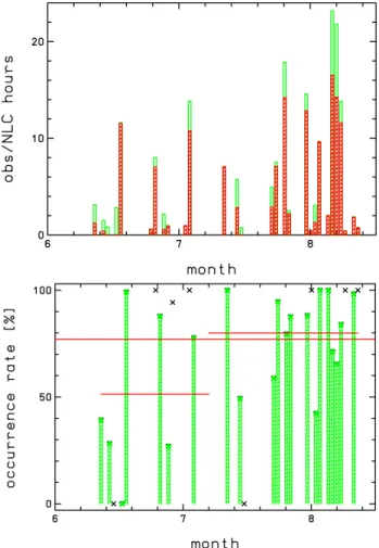
Fig. 2. Daily mean observation statistics for NLC detection by the
K lidar on Spitsbergen. Upper panel: total hours of observation and hours with NLCs (shaded). Lower panel: occurrence frequency of NLCs. Days with little observation time (less than 1 h) are marked by crosses only (no vertical bar). Ignoring these days, 3 mean values have been calculated (horizontal lines): one for the entire period and one each for the period 12 June – 4 July and 12 July – 12 August, respectively.
difference of the actual measurements. An uncertainty in T◦
of ±10 K reduces to ±4, 0.8 and 0.2 K at 90, 85, and 80 km, respectively. A typical overall uncertainty in temperature at 83 km is ±4 K, including errors in T◦and instrumental
ef-fects. The height-dependent sphere reaction time-constant causes a smoothing of the density, temperature, and wind profiles. The smallest scales detectable are typically 8, 3, and 0.8 km at 85, 60, and 40 km, respectively.
3 Observations
3.1 Noctilucent clouds
We have analyzed all available backscatter profiles for NLC and found the first occurrence on the first observation day
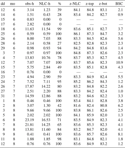
Table 1. Details of the NLCs observed by K lidar in Spitsbergen in the summer of 2001
dd mo obs-h NLC-h % z-NLC z-top z-bot BSC 12 6 3.14 1.23 39 84.1 84.8 83.1 2.1 14 6 1.51 0.43 28 83.4 84.2 82.7 0.9 15 6 0.83 0.00 0 — — — — 17 6 2.82 0.00 0 — — — — 18 6 11.63 11.54 99 83.6 85.1 82.7 3.7 25 6 0.59 0.59 100 86.1 87.3 84.7 3.2 26 6 8.00 7.03 88 83.3 84.5 82.6 5.6 28 6 2.14 0.58 27 82.5 82.8 82.3 2.3 29 6 0.98 0.93 94 84.2 84.8 83.6 1.4 3 7 0.97 0.97 100 84.8 87.3 82.6 2.3 4 7 13.83 10.76 78 83.7 85.3 82.7 4.5 12 7 7.07 7.07 100 83.7 85.6 82.3 10.9 15 7 5.75 2.84 49 83.5 85.1 82.8 4.3 16 7 0.76 0.00 0 — — — — 23 7 4.94 2.90 59 83.3 84.9 82.4 5.5 24 7 7.52 7.11 95 85.2 86.2 84.3 1.2 26 7 17.87 14.22 80 83.2 84.8 82.2 2.6 27 7 2.51 2.20 88 83.3 84.2 82.4 1.0 31 7 14.59 12.86 88 83.2 84.6 82.2 3.3 1 8 0.46 0.46 100 83.4 84.1 82.8 3.8 2 8 3.07 1.30 42 81.6 82.4 80.8 6.2 3 8 9.66 9.66 100 83.8 86.1 82.6 2.5 5 8 2.02 2.02 100 84.1 85.9 82.0 1.3 6 8 23.19 16.53 71 83.5 84.9 82.3 4.1 7 8 21.81 14.25 65 83.6 85.3 82.3 4.1 8 8 13.81 11.60 84 83.2 84.7 82.0 4.1 9 8 0.41 0.41 100 83.6 85.7 82.6 8.1 11 8 1.88 1.85 98 83.1 84.8 82.1 1.8 12 8 0.76 0.76 100 83.6 84.9 83.2 1.2 dd=day; mo=month; obs-h=total observation hours; NLC-h=hours with NLC; %=occurence rate; z-NLC=mean NLC peak altitude; z-top=top of NLC; z-bot=bottom of NLC; BSC=volume backscatter coefficient [10−10/m/sr]
(12 June) and the last on 12 August. Note, that the lidar was out of operation for a significant part of the campaign because of bad weather. The first measurements after 12 Au-gust were made on 26 AuAu-gust and no NLC was observed. In the following we will refer to the time period 12 June until 12 August as the “lidar NLC period”. The total number of observing hours in the lidar NLC period was 184.5 h (5894 profiles) and noctilucent clouds were detected during 142.1 h (4549 profiles), i.e. during 77% of the time. We have ana-lyzed the NLC layers in time slots of 24 h centered around midnight. The result of this analysis is presented in Table 1. As can be seen from Fig. 2 the daily mean occurrence rate varies between 0% (no NLC) and 100% (permanent NLC). Ignoring days with little observation time (i.e. less than 1 h) the scatter of the occurrence rates is ±30%. We have ana-lyzed the daily mean occurrence rates in two subsets, namely in the period 12 June – 4 July, and 12 July – 12 August, respectively. There are 8 days with little observation time
(less than 1 hour). Ignoring these days we find mean occur-rence rates of 51% and 80% with a RMS variability of ±34% and ±19%, respectively. We have also examined the occur-rence frequency in a different manner, namely by summing up all times with and without NLC in the first and second subset (no pre-calculation for each day). Now, the total oc-currence rates are more equal in both subsets: 74% compared to 78%. While strong NLCs (peak BSC>5×10⁻¹⁰/m/sr) are evenly distributed (18/19%), medium NLCs (BSC 2–5) are more frequent in the first period (38/25%) and the occurence of weak NLCs increases (18/35%). At least part of this in-crease is probably due to the fact that the performance of the K lidar was improved throughout the campaign and the solar elevation is lowered which led to a sensitivity increase by a factor of 2–3. We note that more days of observations are available in the second half of the NLC season.
In Fig. 3 the daily mean NLC peak altitudes are shown. Ignoring days where the observation period is less than 1 h
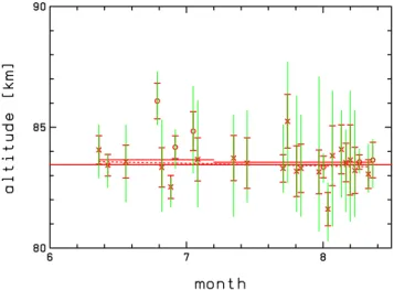
Fig. 3. Daily mean NLC peak altitudes versus month. The crosses
indicate the mean altitude of maximum volume backscatter coeffi-cient βmax(circles if observation time is less than 1 h). The thick
error bars present the RMS variability of βmaxand the thin
verti-cal lines indicate the upper-most and lower-most appearance of the NLC layer during that particular day. The solid horizontal lines give the mean altitudes for the entire period and for the subsets described in the text, respectively. The dashed line is the straight line fitted to the βmaxvalues.
the average NLC peak altitude determined from the daily means is 83.4 km. The mean of all individual NLC peak altitudes (without pre-averaging) is 83.6 km, i.e. practically the same value. This demonstrates that the daily mean al-titudes are representative for the entire data set. The RMS variation of the mean NLC altitude is 1.1 km. The median of the daily NLC peak altitudes is 83.5 km, i.e. very simi-lar to the mean. The distribution of all individual NLC peak altitudes is shown in Fig. 4. The width of the distribution (FWHM) corresponding to a normal distribution is 2.8 km. We have fitted a Gaussian separately to the lower and upper part of the distribution keeping the maximum value at an al-titude of 83 km fixed. We find half widths (FWHM) of 1.9 and 3.5 km, respectively. This indicates that the NLC peak altitudes extend to somewhat higher altitudes above the mean (compared to below). For comparison with measurements at other latitudes we have also determined the centroid altitudes (zc =P(β · z)/ P β) of each NLC profile. The mean of all
these centroid altitudes is of 83.7±1.0 km. Furthermore, we have calculated the “center of half width” defined in Fiedler et al., 2002 and arrive at a mean value of 83.6 km (RMS vari-ability is 1.1 km), again close to the mean of the NLC peak altitudes.
We have analyzed the NLC data in the two subsets men-tioned above and found the mean of the individual NLC peak altitudes at 83.6±0.9 km and 83.5±1.2 km, respectively. This indicates that there is no significant NLC height dif-ference in these subsets which is also evident from the slope
Fig. 4. Histogram of NLC peak altitudes normalized to 100% for
maximum occurrence. The solid vertical lines indicate the mean and the RMS variability of the NLC peak altitudes, respectively.
of a straight line fitted to the daily mean peak altitudes in Fig. 3 which is small (−0.10 km/month) and not significant (uncertainty: ±0.25 km/month). For each NLC profile we have determined the uppermost (“top”) and the lowermost (“bottom”) altitude of the NLC layer. The average top and bottom altitude calculated from all individual NLC profiles is 85.1 and 82.5 km, respectively (RMS variation: ∼1.2 km). The mean layer thickness (FWHM) is 1.7 km (variability: 0.9 km).
The upper edge of the NLC layer is always located be-low the be-lower edge of the potassium layer, as in the exam-ple of Fig. 1. There is no case of a NLC reaching above the lower edge of the potassium layer or appearing (with β >10−10/m/sr) inside. This suggests that there are no very weak NLC present inside the K layer which we could have missed due to the somewhat reduced sensitivity to de-tect NLCs inside the K layer. We therefore argue that our statistics on the altitude and occurrence distribution for weak NLCs is not influenced by the decreased sensitivity inside the K layer.
We have also analyzed the statistical properties of the max-imum volume backscatter coefficient (βmax) at our wave-length of 770 nm. The mean βmaxfor the entire season de-termined from all individual NLC profiles (ignoring profiles with no NLC) is 3.9×10⁻¹⁰/m/sr with a large RMS variabil-ity of nearly 100%. Again, we have analyzed the NLC data in the two subsets mentioned above and found mean values for βmaxof 4.1 and 3.8 with a RMS variability of 3.0 and 4.1, respectively (all values in units of 10−10/m/sr). This implies that there is no significant change of the maximum BSC in these subsets. We note that the measurement of the maxi-mum BSC does not depend on the lidar sensitivity as long as βmaxis significantly above the detection threshold. With the increased sensitivity of the lidar (see above) more weak
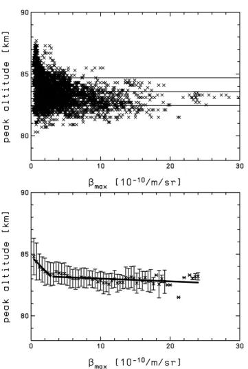
Fig. 5. Scatter plot of the maximum volume backscatter coefficient
βmaxversus peak altitude for all individual profiles (upper panel).
The solid horizontal lines indicate the mean and the RMS variability of the NLC peak altitudes. In the lower panel the peak altitudes are averaged in BSC bins of width 0.4·10−10/m/sr. The vertical lines indicate the variability in each bin. Two straight lines have been fitted (thick solid lines in lower panel) namely for βmaxvalues
smaller and larger than 3, respectively.
NLCs are included in the statistics and a somewhat lower mean value is expected for the second subset.
Another characteristic of NLC layers that can be compared with models is the distribution of βmax with altitude. For example, from steady state considerations of NLC growth and sedimentation it is sometimes taken for granted that the strongest NLCs occur at lowest heights. In Fig. 5a we present a scatter plot of all individual βmaxvalues versus peak alti-tudes. Indeed, there is a weak tendency for brighter NLCs to occur at lower altitudes and this trend varies with βmax. To arrive at more quantitative results we have averaged the peak altitudes in βmax-bins of 0.4×10⁻¹⁰/m/sr and have fit-ted two straight lines, namely for small βmaxvalues (up to 3) and for larger βmax(see Fig. 5b). At small βmaxvalues the slope of a regression line is −0.58±0.08. The slope at larger
Table 2. Simultaneous measurements by K lidar and falling spheres
during ROMA, 2001
flight date, time potassium lidar period NLC label (UT) dates and times (UT)
(ROFS03) 22 Jul. 12:20 22 Jul 23:48–23 Jul 19:47 yes (ROFS05) 25 Jul. 10:00 25 Jul 14:31–26 Jul 14:37 yes ROFS07 31 Jul. 09:00 30 Jul 16:11–31 Jul. 12:00 yes ROFS09 02 Aug. 18:00 02 Aug 08:24–02 Aug 21:45 yes ROFS10 06 Aug. 09:38 05 Aug 09:52–08 Aug 01:54 yes ROFS18 27 Aug. 10:45 26 Aug 09:37–28 Aug 02:00 no
The K lidar time period may include a few hours of data interruption due to bad weather. For ROFS03 and ROFS05 the K
lidar measurements took place a few hours prior to launch.
βmaxvalues is very small (−0.023±0.008) but still statisti-cally significant (all numbers are in the physical dimensions of Fig. 5).
3.2 NLCs and falling sphere temperatures
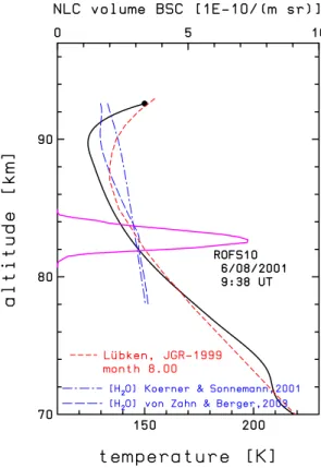
Simultaneous K lidar measurements and FS temperature pro-files are available for 4 flights, where during 3 of these flights a NLC was detected (see Table 2). Two more flights, namely ROFS03 and ROFS05, took place a few hours prior to the closest K lidar measurements and will therefore not be con-sidered in the following discussion. In Fig. 6 we present the temperature profile from ROFS10 and the correspond-ing NLC profile averaged for ±1 h around the rocket launch. Furthermore, two frost point temperature profiles Tfrost are shown using water vapor mixing ratio profiles from two dif-ferent models, namely from K¨orner and Sonnemann (2001) (K&S) and from von Zahn and Berger (2003) (vZ&B). The latter is a 3-dimensional model which includes the effect of freeze drying, i.e. the redistribution of water vapor due to ice particles being formed in the vicinity of the mesopause, and evaporating at lower altitudes. At very high latitudes the two H2O profiles are rather similar up to ∼85 km (difference is less than a factor of 2) but deviate by a factor of up to 10 at the mesopause (see Fig. 9 in von Zahn and Berger, 2003). As can be seen from Fig. 6 the actual temperatures are lower then Tfrostin an extended altitude range from approximately 82 to 91 km (depending on [H2O]) indicating that it is cold enough at these heights for ice particles to grow or to exist. The NLC in Fig. 6 appears at the bottom of the height range where the actual temperatures are smaller than Tfrost. We will come back to a comparison of NLCs and temperatures in Sect. 4.1
Fig. 6. Temperature profile from flight ROFS10 launched on 6
Au-gust at 09:38 UT (black line) and the NLC volume BSC averaged for ±1 h around the rocket launch (purple line; upper abscissa). The two blue dashed lines indicate frost point temperatures Tfrost using model water vapor mixing ratios from K¨orner and Sonne-mann (2001) and from von Zahn and Berger [2003], respectively. For comparison the profile from FJL-JGR99 for 69◦N is presented (red dashed line).
4 Discussion
4.1 NLCs and the degree of saturation
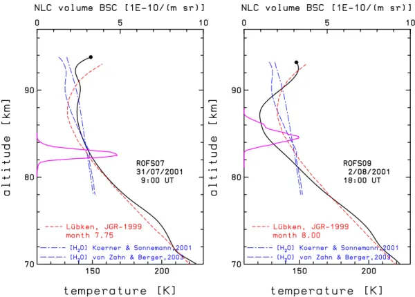
In Fig. 7 two more temperature profiles and the correspond-ing NLC layers are shown, namely from flights ROFS07 and ROFS09. As in Fig. 6 there are various height ranges with super-saturation (Tatm<Tfrost) in the upper mesosphere, but the NLC appears only in the lower part of these height ranges. We have calculated the degree of saturation (S) at the NLC peak and at the top and the bottom of the layer. The results of these calculations are presented in Table 3. To demonstrate the uncertainty of these values due to the un-known water vapor profile we have determined two S values using water vapor values from K&S and vZ&B, respectively. As noted before the two model profiles are rather similar up to ∼85 km and deviate substantially above. Subsequently, the effect on the S values depends on altitude and is substan-tial (more than a factor of 3) only for the NLC top altitude during flight ROFS09. The S values depend strongly on tem-perature (T ), i.e. any error in T results in comparatively large
Table 3. Temperatures in the NLC layer
ROFS07 ROFS09 ROFS10 zt op[km] 84.5 87.3 84.5 temperature [K] 143 121 136 S(K&S) 1.5 1500 13 S(vZ&B) 1.0 140 6 zpeak[km] 82.5 84.5 82.6 βmax[10−10/m/sr] 4.8 3.3 7.3 temperature [K] 149 127 144 S(K&S) 0.5 380 2.3 S(vZ&B) 0.7 180 2.8 zbot t om[km] 80.7 82.9 81.1 temperature [K] 157 137 152 S(K&S) 0.1 18 0.4 S(vZ&B) 0.1 21 0.4
S(K&S) is the degree of saturation using water vapor mixing ratios from K¨orner and Sonnemann (2001).
S(vZ&B) is the degree of saturation using water vapor mixing ratios from von Zahn and Berger (2003).
errors in S. For example, at NLC altitudes an uncertainty in temperature of 2–3 degrees (a typical value at 83 km; see above) corresponds to an uncertainty in S by a factor of 2.
Some of the S values in Table 3 are smaller than one even if we take into account the uncertainties in S discussed above. This suggests that the particles should disappear due to evap-oration. We would like to note, however, that even in a sit-uation of under-saturation it will take some time before an ice particle disappears. For example, with S = 0.5 and a radius of 20 nm it takes several hours before the ice particle has completely evaporated (Gadsden, 1981).
As can be seen from Table 3 the degree of saturation at the NLC peak varies substantially and differs significantly from S = 1. In a simplistic picture one would expect that NLC particles achieve their largest size and produce largest BSC at the S = 1 level since they grow in the S > 1 regime while sedimenting through the atmosphere. However, model stud-ies of microphysical processes controlling the generation of NLCs in the presence of gravity waves have shown that (for long period gravity waves) the NLC peak coincides with the S =1 level only very seldom and values larger and smaller than S = 1 will occur. Rapp et al. (2002) found values in the range of about S = 0.2 to S = 10. Our observations sup-port this finding even if we take into account the uncertainties about the actual S value discussed above.
For flight ROFS07 a major part of the NLC is located in a region of under-saturation in particular at the bottom of the layer at 80.7 km. We note that large enhancements of water vapor up to 10-15 ppmv have been observed in this altitude range by the HALOE instrument on UARS, though at lower latitudes Summers et al. (2001). This enhancement is
pre-Fig. 7. Same as pre-Fig. 6 but for flights ROFS07 (left panel) and ROFS09 (right panel). The launch dates and times are given in the plots.
sumably caused by the “freeze drying” effect mentioned ear-lier We can certainly not exclude that the local water vapor concentration during flight ROFS07 deviated largely from the model values. For flight ROFS09, very large S values are found in the entire NLC layer. We conclude that the range of S values in the NLC layer varies greatly and can be larger and smaller than one.
As can also be seen from Table 3 there is no obvious correlation between the degree of saturation and the maxi-mum volume backscatter coefficient βmax. The peak BSC varies only little and is largest in a case of moderate super-saturation (S = 2 for flight ROFS10). This again supports the statement that arguments derived from steady-state as-sumptions may not be applicable when relating individual NLC properties to the background thermal field. On the other hand, the mean variation of the NLC appearance with height and season is in agreement with the climatological variation of super-saturation derived from the FS temperature mea-surements (see Fig. 4 in L¨ubken and M¨ullemann, 2003). This is true even if we consider the uncertainty S caused by the unknown water vapor concentration discussed above. At the end of our lidar NLC period (12 August, i.e. when measure-ments had to be terminated due to bad weather) temperatures are still low enough for super-saturation. When the lidar was started again on 26 August temperatures had just become too high for super-saturation and indeed no NLC was observed.
The maximum S values deduced from the FS climatology occur around 87–88 km and reach values of 26, 3, and 0.2 for 15 August, 23 August, and 1 September, respectively, us-ing H2O values from K&S. Similar values for the model of vZ&B can not be given because this model depends not on season. This indicates that at 26 August (time = 8.84) clima-tological temperatures are too high for the creation of NLCs. We conclude that there is a very close correspondence of the general morphology of NLCs and the local thermal structure over Spitsbergen allowing for super-saturation, in spite of the large time constants (hours) which are associated with large horizontal transport distances (Berger and von Zahn, 2002).
In summary, NLCs appear in the lower part of the height range of super-saturation but details of their morphology (BSC, layer width etc.) do not depend on the local thermal structure. This is in line with model results which suggest that it can take several hours before an ice particle reaches a size detectable by lidar (Berger and von Zahn, 2002; Rapp et al., 2002). During this time the particle is carried hundreds of kilometers by the mean wind and the background con-ditions relevant for ice particle formation, e.g. temperatures and vertical winds, have most likely varied. On the other hand, the mean variation of the NLC appearance with height and season is in nice agreement with the climatological vari-ation of the thermal structure in the upper mesosphere.
4.2 Comparison of NLCs with other latitudes
The characteristics of NLCs observed by the R/M/R-lidar at ALOMAR (69◦N) have recently been summarized by Fiedler et al. (2002) based on data from 5 summer seasons. Technical details of the lidar are described in von Zahn et al. (2000). Although our statistics are poorer compared to ALO-MAR we will now compare the main NLC features at both sites. The analysis of Fiedler et al. was performed in 5 time periods of 15 days each. Our lidar NLC period at Spitsber-gen is best represented by their periods 2–5 (16 June – 15 August).
The NLC occurrence frequency at ALOMAR varies from year to year and is in the range ∼30–50%. This is consid-erably less compared to Spitsbergen (77%). In the year of our measurements (2001) the mean occurrence frequency at ALOMAR is 28% which is less than half compared to Spits-bergen. To avoid an instrumental bias in these values we compare the rates derived for NLCs which are stronger than a threshold of βmax>4 which is clearly above the detection limit of the ALOMAR lidar. The occurence rate then ranges between 20 and 30%, with the lower value observed in 2001. Using a corresponding threshold of βmax>1.25 at 770 nm (see below), which is above our instrumental limit, we obtain an occurence rate of 61%, again more than twice the value from 69◦N. This occurrence increase of NLCs with latitude is in line with the increase of polar mesospheric cloud (PMC) frequency observed by satellites (Thomas et al., 1991).
The mean center NLC altitude zcat ALOMAR varies
lit-tle in periods 2–5 and is approximately 83.3 km (variabil-ity: ±1.2 km) which is very similar to our value of 83.6 km. The center altitude at ALOMAR has increased since 1997 and reaches ∼83.9 km in 2001, thus varying about the value at Svalbard. Fiedler et al. (2002) find only very little sea-sonal variation of zc, again very similar to our observations
at Spitsbergen. The mean width of 1.3 km at ALOMAR is slightly less compared to Spitsbergen (1.7 km).
The maximum BSC at ALOMAR has decreased since 1997 and reached a mean of βmax= 9· 10−10/m/sr in 2001. This value is slightly larger (9.6) if the same time period in 2001 is taken at ALOMAR compared to our campaign period at Spitsbergen. Please note that there exist large differences between mean, median and mode values for βmaxas is de-scribed in more detail in Fiedler et al. (2002).
When comparing NLC strengths measured by different li-dars the wavelength dependence of the backscatter coeffi-cient must be taken into account. The ratio of the BSCs at two wavelengths is called “color ratio” and depends strongly on the particle mode radius rm and on the size distribution.
We assume a lognormal size distribution of spherical ice par-ticles with rm = 40 nm and a width of σ = 1.4. We
then arrive at color ratios of 3.2 and 7.3 for 532 nm/770 nm and 374 nm/770 nm, respectively. These ratios need to be applied for the comparison of our results with the R/M/R-lidar at ALOMAR and the Fe R/M/R-lidar at the South pole (see
later). Taking into account this color ratio the ALOMAR value of βmax= 9.6 (see above) corresponds to a βmax of 3.0·10−10/m/sr at 770 nm which is slightly but not signif-icantly less compared to the Spitsbergen mean of βmax= 3.9·10−10/m/sr. We note that the color ratio varies substan-tially (from approximately 2.5 – 4.5) if other particle radii and widths are assumed. Therefore we conclude, that the brightness of the NLCs at ALOMAR and at Spitsbergen do not deviate significantly.
In summary, the mean NLC characteristics at two sites separated by almost 10 degrees in latitude, namely ALO-MAR at 69◦N and Spitsbergen at 78◦N, are similar with re-spect to the peak altitude and the maximum volume backscat-ter coefficient, but differ significantly with respect to the oc-currence frequency (larger at higher latitudes).
Chu et al. (2002) have recently presented NLC results obtained with their Fe Boltzmann lidar (374 nm) at the South Pole during the summer seasons of 1999/2000 and 2000/2001. Their coverage of the summer season is simi-lar to our “lidar NLC period” (12 June to 12 August which corresponds to day numbers after solstice of −9 and 52, re-spectively) with a somewhat better coverage at the beginning of the NLC season. Taking mean values from both years the centroid altitude zc at the South pole is approximately
85.0 km, i.e. ∼1.3 km higher compared to Spitsbergen. It should be noted, however, that zc varies by approximately
1 km in the two years of observations at the South pole. We do not detect a decrease of NLC altitudes at the end of the season as stated in Chu et al. (2002). The NLC occurrence frequency at the South pole is somewhat smaller (67%) com-pared to Spitsbergen, but the difference is within the natural variability observed during our NLC season (±28%).
The mean of the maximum backscatter coefficients βmax at the South pole is 37·10−10/m/sr at 374 nm. This corre-sponds to 5.1 at 770 nm taking the color ratio into account (see above). This is somewhat larger compared to the mean value at Spitsbergen (3.9). However, the difference is within the uncertainty of the color ratio caused by the unknown mean particle radius and size distribution.
5 Conclusion and outlook
We have presented the first lidar observations of noctilucent clouds at Spitsbergen and have discussed in detail the sta-tistical properties of the NLC layer height, strength etc. We have compared these results with the thermal structure of the background field deduced from falling sphere measurements. The NLC altitudes and strengths at Spitsbergen are similar to ALOMAR (10◦ further south) but NLCs are more frequent
at Spitsbergen.
The comparison of FS temperatures and NLCs demon-strates that arguments derived from steady-state assumption may not be applicable when relating individual NLC prop-erties to the background thermal field. On the other hand,
the mean variation of the NLC appearance with height and season is in nice agreement with the climatological variation of the thermal structure in the upper mesosphere. This lo-cal agreement between the mean appearance of NLCs and the conditions set by the background atmosphere is important for comparison with models which take into account the time constant of hours for the generation of NLC particles and the corresponding large horizontal transport distances. We will continue and complete our measurements in the next years to explore inter-annual variability and improve the statistics of NLCs at very high latitudes.
Acknowledgements. We thank Mrs. Liu, Mr. Menzel, and Mr.
Laut-enbach for their assistance during the lidar operation. The support of the Svalsat team during installation and maintenance of the lidar in Spitsbergen is gratefully acknowledged. We thank A. M¨ullemann for the FS data processing and G. Baumgarten and M. Alpers for the color ratio calculations. J. Fiedler has kindly provided results for the comparison with the ALOMAR data. The ROMA project is supported by the Bundesministerium f¨ur Bildung, Wissenschaft, Forschung und Technologie, Bonn, under grants 50 OE 99 01 and 07 ATF 10.
References
Alpers, M., Gerding, M., H¨offner, J., and von Zahn, U.: NLC parti-cle properties from a five-color observation at 54◦N, J. Geophys. Res., 105, 12 235–12 240, 2000.
Baumgarten, G., L¨ubken, F. J., and Fricke, K. H.: First observation of one noctilucent cloud by a twin lidar in two different direc-tions, Ann. Geophysicae, 20, 1863–1868, 2002.
Berger, U. and von Zahn, U.: Icy particles in the summer mesopause region: 3-dim modeling of their environment and 2-dim modeling of their transport, J. Geophys. Res., 107, doi. 10.1029/2001JA00316, 2002.
Chu, X., Gardner, C., and Papen, G.: Lidar observations of polar mesospheric clouds at south pole: seasonal variations, Geophys. Res. Lett., 28, 1203–1206, 2001.
Chu, X., Gardner, C., and Roble, R.: Lidar studies of inter-annual, seasonal and diurnal variations of polar mesospheric clouds at the South pole, J. Geophys. Res., 108, 8447, doi. 10.1029/2002JD002524, 2002.
Fiedler, F., Baumgarten, G., and von Cossart, G.: Noctilucent clouds above ALOMAR between 1997 and 2001: Occurrence and properties, J. Geophys. Res., doi. 10.1029/2002JD002419, 2002.
Fleming, E. L., Chandra, S., Barnett, J. J., and Corney, M.: Zonal mean temperature, pressure, zonal wind, and geopotential height as functions of latitude, Adv. Space Res., 10, 12, 11–59, 1990. Fricke-Begemann, C., Alpers, M., and H¨offner, J.: Daylight
rejec-tion with a new receiver for potassium resonance temperature lidars, Opt. Lett., 27, 21, 1932–1934, 2002.
Fritts, D. C., Isler, J. R., Thomas, G. E., and Andreassen, Ø.: Wave breaking signatures in noctilucent clouds, Geophys. Res. Lett., 20, 2039–2042, 1993.
Gadsden, M.: The north-west Europe data on noctilucent clouds: a survey, J. Atmos. Sol.-Terr. Phys., 60, 1163–1174, 1998.
Gadsden, M. and Schr¨oder, W.: Noctilucent clouds, Springer-Verlag, New York, 1989.
Gadsden, M.: The silver-blue cloudlets again: nucleation and growth of ice in the mesosphere, Planet. Space Sci., 29, 1079– 1087, 1981.
Garcia, R. R.: Dynamics, radiation and photochemistry in the meso-sphere: Implications for the formation of noctilucent clouds, J. Geophys. Res., 94, 14 605–14 615, 1989.
Hansen, G., Serwazi, M., and von Zahn, U.: First detection of a noctilucent cloud by lidar, Geophys. Res. Lett., 16, 1445–1448, 1989.
Jensen, E. and Thomas, G. E.: A growth-sedimentation model of polar mesospheric clouds: Comparions with SME measure-ments, J. Geophys. Res., 93, 2461–2473, 1988.
Jesse, O.: Die leuchtenden Nachtwolken, Meteorol. Zeitung, 6, 184–186, 1889.
Kirkwood, S. and Stebel, K.: The influence of planetary waves on noctilucent cloud occurrence over NW Europe, J. Geophys. Res., 108, doi. 10.1029/2002JD002356, 2003.
Klostermeyer, J.: A simple model of the ice particle size distribu-tion in noctilucent clouds, J. Geophys. Res., 103, 28 743–28 752, 1998.
K¨orner, U. and Sonnemann, G. R.: Global 3D-modeling of the wa-ter vapor concentration of the mesosphere/mesopause region and implications with respect to the NLC region, J. Geophys. Res., 106, 9639–9651, 2001.
Leslie, R.: Sky glows, Nature, 32, 245, 1885.
L¨ubken, F.-J.: Thermal structure of the Arctic summer mesosphere, J. Geophys. Res., 104, 9135–9149, 1999.
L¨ubken, F.-J.: Nearly zero temperature trend in the polar summer mesosphere, Geophys. Res. Lett., 27, 3603–3606, 2000. L¨ubken, F.-J. and M¨ullemann, A.: First in situ temperature
measure-ments in the summer mesosphere at very high latitudes (78◦N), J. Geophys. Res., 108, doi. 10.1029/2002JD002414, 2003. L¨ubken, F.-J., Hillert, W., Lehmacher, G., von Zahn, U., Bittner, M.,
Offermann, D., Schmidlin, F., Hauchecorne, A., Mourier, M., and Czechowsky, P.: Intercomparison of density and tempera-ture profiles obtained by lidar, ionization gauges, falling spheres, datasondes, and radiosondes during the DYANA campaign, J. At-mos. Terr. Phys., 56, 1969–1984, 1994.
L¨ubken, F.-J., Fricke, K.-H., and Langer, M.: Noctilucent clouds and the thermal structure near the Arctic mesopause, J. Geophys. Res., 101, 9489–9508, 1996.
L¨ubken, F.-J., H¨offner, J., Fricke-Begemann, C., M¨ullemann, A., Zecha, M., and R¨ottger, J.: Mesospheric layers and tempera-tures at Spitsbergen, 78◦N, in Proceedings of the “Mesospheric Clouds” meeting, edited by Gadsden, M., British Astronomical Association, Perth, Scottland, 2002.
Rapp, M., L¨ubken, F.-J., M¨ullemann, A., Thomas, G. E., and Jensen, E. J.: Small scale temperature variations in the vicin-ity of NLC: Experimental and model results, J. Geophys. Res., 107, doi. 10.1029/2001JD001241, 2002.
Schmidlin, F. J.: The inflatable sphere: A technique for the accurate measurement of middle atmosphere temperatures, J. Geophys. Res., 96, 22,673–22,682, 1991.
Summers, M. E., Conway, R. R., Englert, C. R., Siskind, D. E., Stevens, M. H., Russell, J. M., Gordley, L. L., and McHugh, M. J.: Discovery of a water vapor layer in the Artic summer mesosphere: Implications for Polar mesospheric clouds,
Geo-phys. Res. Lett., 28, 3601–3604, 2001.
Thayer, J., Rapp, M., Gerrard, A., Gudmundsson, E., and Kane, T.: Grawity Wave Influences on Arctic Mesospheric Clouds as Determined by the Sondrestrom, Greenland, Rayleigh Lidar, J. Geophys. Res., 107, doi. 10.1029/2002JD002363, 2002. Thomas, G. E., Olivero, J. J., Jensen, E. J., Schroeder, W., and Toon,
O. B.: Relation between increasing methane and the presence of ice clouds at the mesopause, Nature, 338, 490–492, 1989. Thomas, G. E., McPeters, R. D., and Jensen, E. J.: Satellite
obser-vations of polar mesospheric clouds by the solar backscattered ultraviolet spectral radiometer: evidence of a solar cycle depen-dence, J. Geophys. Res., 96, 927–939, 1991.
von Cossart, G., Fiedler, J., and von Zahn, U.: Size distributions of NLC particles as determined from 3-color observations of NLC by ground-based lidar, Geophys. Res. Lett., 26, 1513–1516, 1999.
von Zahn, U. and Berger, U.: Persistent ice cloud in the midsummer upper mesosphere at high latitudes: Three-dimensional model-ing and cloud interactions with ambient water vapor, J. Geophys. Res., 108, 8451, doi. 10.1029/2002JD002409, 2003.
von Zahn, U. and H¨offner, J.: Mesopause temperature profiling by potassium lidar, Geophys. Res. Lett., 23, 141–144, 1996. von Zahn, U. and Meyer, W.: Mesopause temperatures in polar
summer, J. Geophys. Res., 94, 14 647–14 651, 1989.
von Zahn, U., von Cossart, G., and Fiedler, J.: Tidal variations of noctilucent clouds measured at 69◦N latitude by ground based lidar, Geophys. Res. Lett., 25, 1289–1292, 1998.
von Zahn, U., von Cossart, G., Fiedler, J., Fricke, K. H., Nelke, G., Baumgarten, G., Rees, D., Hauchecorne, A., and Adolfsen, K.: The ALOMAR Rayleigh/Mie/Raman lidar: Objectives, configu-ration, and performance, Ann. Geophysicae, 18, 815–833, 2000.