Modeling place cells and grid cells in multi-compartment environments: Entorhinal–hippocampal loop as a multisensory integration circuit

HAL Id: hal-03062697

https://hal.archives-ouvertes.fr/hal-03062697

Submitted on 14 Dec 2020

HAL is a multi-disciplinary open access

archive for the deposit and dissemination of

sci-entific research documents, whether they are

pub-lished or not. The documents may come from

teaching and research institutions in France or

abroad, or from public or private research centers.

L’archive ouverte pluridisciplinaire HAL, est

destinée au dépôt et à la diffusion de documents

scientifiques de niveau recherche, publiés ou non,

émanant des établissements d’enseignement et de

recherche français ou étrangers, des laboratoires

publics ou privés.

Modeling place cells and grid cells in multi-compartment

environments: Entorhinal–hippocampal loop as a

multisensory integration circuit

Tianyi Li, Angelo Arleo, Denis Sheynikhovich

To cite this version:

Tianyi Li, Angelo Arleo, Denis Sheynikhovich.

Modeling place cells and grid cells in

multi-compartment environments: Entorhinal–hippocampal loop as a multisensory integration circuit.

Neu-ral Networks, Elsevier, 2020, 121, pp.37-51. �10.1016/j.neunet.2019.09.002�. �hal-03062697�

Neural Networks 121 (2020) 37–51

Contents lists available atScienceDirect

Neural Networks

journal homepage:www.elsevier.com/locate/neunet

Modeling place cells and grid cells in multi-compartment

environments: Entorhinal–hippocampal loop as a multisensory

integration circuit

Tianyi Li, Angelo Arleo, Denis Sheynikhovich

∗

Sorbonne Université, INSERM, CNRS, Institut de la Vision, 17 rue Moreau, F-75012 Paris, France

a r t i c l e i n f o

Article history:

Received 8 April 2019

Received in revised form 24 July 2019 Accepted 2 September 2019 Available online 6 September 2019

Keywords: Place cells Grid cells Multisensory integration Hippocampus Computational model Neural network a b s t r a c t

Hippocampal place cells and entorhinal grid cells are thought to form a representation of space by integrating internal and external sensory cues. Experimental data show that different subsets of place cells are controlled by vision, self-motion or a combination of both. Moreover, recent studies in environments with a high degree of visual aliasing suggest that a continuous interaction between place cells and grid cells can result in a deformation of hexagonal grids or in a progressive loss of visual cue control over grid fields. The computational nature of such a bidirectional interaction remains unclear. In this work we present a neural network model of the dynamic interaction between place cells and grid cells within the entorhinal–hippocampal processing loop. The model was tested in two recent experimental paradigms involving environments with visually similar compartments that provided conflicting evidence about visual cue control over self-motion-based spatial codes. Analysis of the model behavior suggests that the strength of entorhinal–hippocampal dynamical loop is the key parameter governing differential cue control in multi-compartment environments. Moreover, con-struction of separate spatial representations of visually identical compartments required a progressive weakening of visual cue control over place fields in favor of self-motion based mechanisms. More generally our results suggest a functional segregation between plastic and dynamic processes in hippocampal processing.

© 2019 The Author(s). Published by Elsevier Ltd. This is an open access article under the CC BY license (http://creativecommons.org/licenses/by/4.0/).

1. Introduction

It has long been accepted that spatial navigation depends cru-cially on a combination of visual and self-motion input (O’Keefe & Nadel,1978). Since the seminal work ofO’Keefe and Dostro-vsky (1971), a neural locus of this combination is thought to be the place cell network in the CA1–CA3 subfields of the hip-pocampus proper (Jayakumar et al., 2019; Knierim, Kudrimoti, & McNaughton, 1998; Muller & Kubie,1987; O’Keefe & Speak-man, 1987), with different subsets of place cells sensitive to self-motion cues, to visual cues or, more often, to a combination of them (Chen, King, Burgess, & O’Keefe, 2013; Fattahi, Sharif, Geiller, & Royer, 2018; Markus, Barnes, McNaughton, Gladden, & Skaggs, 1994). A more recent discovery of grid cells in the medial entorhinal cortex (mEC) led to the suggestion that the grid-cell network provides a self-motion-based representation of location that is combined with other sensory information on the level of place cells (Cheng & Frank, 2011; Fyhn, Molden,

∗

Corresponding author.

E-mail addresses: tianyi.li@inserm.fr(T. Li),angelo.arleo@inserm.fr

(A. Arleo),denis.sheynikhovich@upmc.fr(D. Sheynikhovich).

Witter, Moser, & Moser, 2004; Hayman & Jeffery, 2008; Jacob, Capitano, Poucet, Save, & Sargolini,2019;McNaughton, Battaglia, Jensen, Moser, & Moser, 2006). The grid-cell representation is itself vision-dependent, since various properties of grid cells are affected by changes in visual features of the environment ( Haft-ing, Fyhn, Molden, Moser, & Moser,2005;Krupic, Bauza, Burton, Barry, & O’Keefe, 2015). Combined with the evidence showing that coherent changes in place-cell and grid-cell representations occur during environment deformation and cue manipulation, these data suggest a bidirectional interaction between these rep-resentations at the neural level (Fyhn, Hafting, Treves, Moser, & Moser,2007). While this bidirectional link is always present in normal conditions, it may not be necessary for place cell activities, as shown in a number of lesion experiments (Sasaki, Leutgeb, & Leutgeb,2015;Schlesiger, Boublil, Hales, Leutgeb, & Leutgeb, 2018).

The nature of the dynamic interaction between visual and self-motion cues on the level of grid cells has recently been tested in two experiments: in a merged room, formed by removal of a wall separating two visually similar environments (Wernle et al., 2018), and during exploration of an environment consisting of two identical rooms connected by a corridor (Carpenter, Manson, https://doi.org/10.1016/j.neunet.2019.09.002

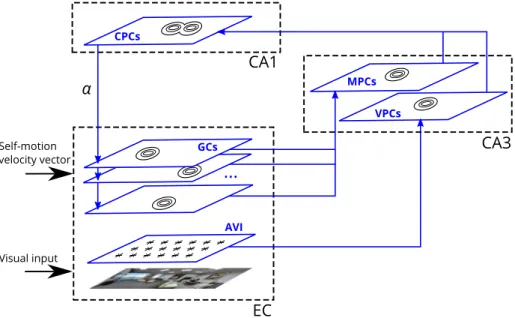
Fig. 1. Schematic representation of the model. Self-motion input is integrated in 5 grid-cell populations of the medial EC (only 3 populations are shown for clarity), and via competitive interactions results in a self-motion-driven space representation in CA3 (encoded by the MPC population). Visual input, represented by the activities of AVI neurons, results in a purely vision-based representation in CA3, encoded by the VPC population. Both MPCs and VPCs project to CA1 where the conjunctive representation of location is encoded in the CPC population. The projection from CPCs in CA1 back to the mEC closes the dynamic hippocampal processing loop and the strength of this projection is determined by the parameterα. The arrows represent the information flow in the network. Small ovals represent subsets of strongly active cells in the corresponding populations (even though strongly active cells are shown in nearby locations in the figure, no particular topographical relations between cells are assumed in the model, apart from the AVI population with a retinotopic neuronal organization).

Jeffery, Burgess, & Barry,2015). Results of the first experiment have shown that firing patterns of grid cells were anchored by local sensory cues near environmental boundaries, while they underwent a continuous deformation far from the boundaries in the merged room, suggesting a strong control of local visual cues over the grid-cell representation (Wernle et al.,2018). Results of the second experiment indicated in contrast that during learning in a double-room environment grid cells progressively formed a global self-motion-based representation disregarding previously learned local visual cues (Carpenter et al.,2015).

Existing models of the entorhinal–hippocampal system are mostly based on the feed-forward input from grid cells to place cells, with an additional possibility to reset grid-field map upon the entry to a novel environment (Blair, Gupta, & Zhang,2008; O’Keefe & Burgess,2005;Pilly & Grossberg,2012;Sheynikhovich, Chavarriaga, Strösslin, Arleo, & Gerstner,2009;Solstad, Moser, & Einevoll, 2006), or focus on the feed-forward input from place cells to grid cells (Bonnevie et al., 2013). In addition to be at difficulty at explaining the above results on dynamic interac-tions between visual and self-motion cues, they are also not consistent with data showing that hippocampal spatial represen-tations remain spatially tuned after mEC inactivation (Brun et al., 2008;Rueckemann et al.,2016), that in rat pups place fields can exist before the emergence of the grid cell network (Muessig, Hauser, Wills, & Cacucci,2015) and that disruption of grid cell spatial periodicity in adult rats does not alter preexisting place fields nor prevent the emergence of place fields in novel envi-ronments (Brandon, Koenig, Leutgeb, & Leutgeb, 2014; Koenig, Linder, Leutgeb, & Leutgeb,2011).

In this paper we propose a model of continuous dynamic loop-like interaction between grid cells and place cells, in which the main functional parameter is the feedback strength in the loop. We show that the model is able to explain the observed pattern of grid-cell adaptation in multi-compartment environments by as-suming a progressive decrease of visual control over self motion, and a plasticity mechanism regulated by allothetic and idiothetic cue mismatch over a long time scale.

2. Model

The rat is modeled by a panoramic visual camera moving in an environment along quasi-random trajectories resembling those of a real rat. The orientation of the camera corresponds to the head orientation of the model animal. The constant speed of the modeled rat is set to 10 cm/s, and sampling of sensory input oc-curs at frequency 10 Hz, roughly representing hippocampal theta update cycles. The modeled rat receives two types of sensory input (Fig. 1). First, self-motion input to the model is represented by angular and translational movement velocities integrated by grid cells in mEC to provide self-motion representation of loca-tion, as proposed earlier (McNaughton et al.,2006). Competitive self-organization of grid cell output occurs downstream from the entorhinal cortex in the dentate gyrus (DG)–CA3 circuit and gives rise to a self-motion-based representation of location, encoded by motion-based place cells (MPC). We did not include a specific neuronal population to model DG (see, e.g.,de Almeida, Idiart, & Lisman,2009b). Instead, we implemented competitive learning directly on mEC inputs to CA3. Second, visual input is represented by responses of a two-dimensional retina-like grid of orientation-sensitive Gabor filters, applied to input camera images at each time step. For instance, in featureless rectangular rooms used in most of the simulations below, the only features present in the input images are the outlines of the environment walls (Fig. 2A, bottom). Importantly, the ‘retinal’ responses are assumed to be aligned with an allocentric directional frame further along the dorsal visual pathway (not modeled), the directional frame be-ing set by head direction cells (Byrne, Becker, & Burgess,2007; Sheynikhovich et al., 2009). That is, visual input to the model at each spatial location is independent on the head direction that the model rat has upon arriving at that location. The visual input aligned with an allocentric directional frame is assumed to be encoded in the inputs to the hippocampal formation from non-grid mEC cells or from the lateral entorhinal cortex (lEC). Competitive self-organization of these inputs results in a purely vision-based representation of location, encoded by a population of visual place cells (VPCs). Both MPCs and VPCs project to CA1

T. Li, A. Arleo and D. Sheynikhovich / Neural Networks 121 (2020) 37–51 39

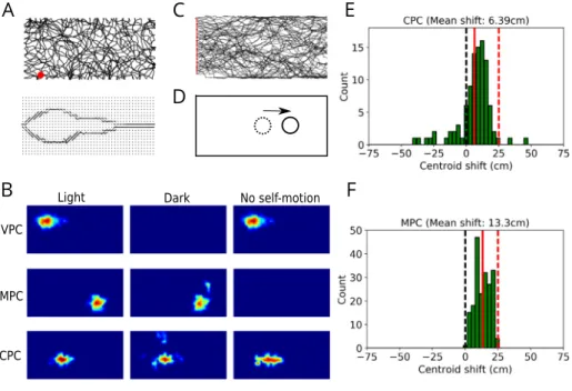
Fig. 2. Multisensory integration in modeled place cells. A. An example of the trajectory of the modeled animal in a rectangular environment (top) and the visual input to the model (bottom) from the location marked by the red dot. In the bottom plot, the dots represent the grid of Gabor filters, and lines represent the orientations of the most active filters. Visual input at each location is independent from head direction. B. Firing fields of VPCs (top row), MPCs (middle row) and CPCs (bottom row) in simulated ‘light’ condition (left column), ‘dark’ condition (middle column) and during passive translation (right column). C. Trajectories of model animal crossing the rectangular environment from left to right. The red dots denote the starting positions. D. When the model rat crosses the environment from left to right, self-motion position estimate (dotted circle) is behind the visual position estimate (full circle) in the conditions of decreased speed gain, leading to a forward-shift of receptive fields. E,F. Forward-shift of receptive fields in the population of CPCs (top) and MPCs (bottom). Full red lines represent the mean shift in the population. Dashed red lines represent the shift due to purely self-motion input.

cells that form a conjunctive representation of location in

con-junctive place cells (CPCs). The CPCs in CA1 project back to the

entorhinal grid cells and thus form a recurrent loop, reflecting the anatomy of entorhinal–hippocampal connections (Iijima et al., 1996). Further details of the model components and synaptic learning rules are described in the following sections.

2.1. Visual input

Visual snapshots of the environment are produced by a panoramic cylindrical camera representing the model rat visual field (160◦

x 360◦

). These snapshots are then encoded by the activities of a rectangular sheet of 40

×

90 neurons uniformly covering the visual field. The activities of visual neurons are computed in four steps. First, input images are convolved with Gabor filters of 4 different orientations (0

,

90◦

_,

180◦

_,

270◦

) at 2 spatial frequencies (0.5 cpd, 2.5 cpd), chosen so as to detect visual features of simulated environments (see Section3). Second, the 8 convolution images are discretized with the 40

×

90 grid, and the maximal response at each position is chosen, producing an array of 3600 filter responses. These operations are assumed to roughly mimic retinotopic V1 processing. Third, the filter responses are aligned with a common allocentric directional frame (assumed to be given by the head direction system), such that if the model rat rotates without changing its spatial location, the activities of aligned filters stay constant. This operation implements an egocentric–allocentric coordinate transformation thought to be performed by parietal cortex neurons (Byrne et al.,2007). Fourth, the vector of aligned filter activities at time t is normalized to length unity, giving the final neuronal activities Aavi(t

,

j) of the

allocentric visual input cells, with the index j running over all elements of the vector.

2.2. Integration of visual and self-motion input by grid cells

The self-motion input is processed by 5 identical neuronal populations (seeFig. 1) representing distinct grid-cell populations in the dorsal mEC (Hafting et al.,2005). Each grid cell population is modeled by a two-dimensional sheet of neurons equipped with attractor dynamics on a twisted-torus topology, as has been proposed in earlier models (Burak & Fiete,2009;Guanella, Kiper, & Vershure,2007;Sheynikhovich et al.,2009). The position of an attractor state (corresponding to subset of strongly active cells, or activity packet) in each grid-cell population is updated based on the self-motion velocity vector. This is implemented by the modulation of recurrent connection weights with Mexican hat-like structure (i.e. with short-range excitation and long-range inhibition) according to the model rat rotation and displacement, such that the activity packet moves across the neural sheet ac-cording to the rat movements in space (Guanella et al.,2007). The only difference between different grid-cell populations is that the speed of movement of the activity packet across the neural sheet is specific for each population, resulting in a population-specific distance between neighboring grid fields and field size ( Haft-ing et al., 2005). As long as each location in an environment corresponds to a distinct combination of positions of the activ-ity packets, the population activactiv-ity of all grid cells encodes the current position of the animal in the environment (Fiete, Burak, & Brookings, 2008). The exact implementation of the attractor mechanism governing grid-cell network dynamics is not essential for our model to work.

In addition to the recurrent input from other grid cells in the same population, each grid cell receives input from the CPC pop-ulation which represent conjunctive visual and self-motion rep-resentation (described in detail later), and the relative strength of these two inputs is controlled by the parameter

α

. At a relatively

high value of this parameter, the position of the activity packet in each grid-cell layer is strongly influenced by the hippocampal in-put, leading to an overall stronger effect of visual information. At a low value of

α

, the position of the attractor states is determined exclusively by the self-motion input.

Thus, the total synaptic input to grid cell i at time t is (omitting grid cell population index for clarity)

Igc(t

,

i)

=

α

Igccpc(t

,

i)

+

(1

−

α

)Igcgc(t

,

i) (1)

where the external input from CPCs and the recurrent input from other grid cells are determined by

I_gccpc(t

,

i)

=

ncpc

∑

j=1 Acpc(t

−

1

,

j)Wgccpc(t

,

i

,

j) (2) I_gcgc(t

,

i)

=

ngc

∑

k=1 Agc(t

−

1

,

k)Wgcgc(t

,

i

,

k) (3)

Here, Acpc(t

,

j) is the activity of jth CPC at time t (described below)

and Agc(t

,

k)

=

Igc(t

,

k) is the activity of kth grid cell (we use

linear activation function for grid cells).

Feedforward synaptic connections from CPCs are initialized by small random values and updated during learning according to a standard Hebbian learning scheme:

W_gccpc(t

,

i

,

j)

=

W_gccpc(t

−

1

,

i

,

j)

+

η

cpc_gc Agc(t

,

i)Acpc(t

,

j) (4)

followed by explicit normalization ensuring that the norm of the synaptic weight vector of each cell is unity.

Recurrent synaptic connections between grid cells are con-structed such as to ensure attractor dynamics, modulated by velocity vector (Guanella et al.,2007). More specifically, the con-nection weight between cells i and j is a Gaussian function of the distance between these cells in the neural sheet. This connection weight is modulated by the self-motion velocity vector, such that the activity packet moves across the neural sheet according to the direction and norm of the velocity vector, with a proportionality constant that is grid-cell population specific. These proportion-ality constants were tuned such that the grid spacing across different grid cell populations were between 42 cm and 172 cm. Grid-cell firing patterns were oriented 7.5◦

with respect to one of the walls of an experienced experimental enclosure (Krupic et al., 2015).

2.3. Encoding of visual and self-motion input by place cells

As mentioned above, the model includes three distinct popula-tions of place cells (Fig. 1). First, VPCs directly integrate allocentric visual inputs and project further to CA1. We putatively assign VPC population to CA3 where a competitive mechanism based on recurrent feedback can result in self-organization of visual inputs, the resulting spatial code further transmitted to CA1. The model of this pathway is based on the evidence that stable spatial rep-resentations were observed in CA1 after complete lesions of the mEC containing grid cells (Brandon et al.,2014;Schlesiger et al., 2018). Second, MPCs directly integrate input from grid cells and in the absence of visual inputs the activity of these cells repre-sents purely self-motion-based representation of location. These cells represent CA3 place cells, acquiring their spatial selectivity via a competitive mechanism based on mEC inputs. Third, CPCs that model CA1 pyramidal cells, combine visual and self-motion inputs coming from VPC and MPC populations, respectively. Cru-cially, CPCs project back to the grid cell populations, modeling anatomical projections from CA1 back to the entorhinal cortex forming a loop (Iijima et al.,1996;Slomianka, Amrein, Knuesel, Sørensen, & Wolfer,2011) and controlled by the parameter

α

as described above.

Vision-based place cells. VPCs acquire their spatial selectivity

as a result of unsupervised competitive learning implemented directly on the allocentric visual inputs (see Section2.1). Thus, the total input to a VPC i at time t is given by

Iavi vpc(t

,

i)

=

navi

∑

j=1 Aavi(t

,

j)W_vapcvi(t

,

i

,

j) (5)

where Aavi(t

,

j) is the activity of jth Gabor filter aligned with

the allocentric directional frame. To compute output activities

A_vpc(t

,

i) of the VPC cells, (i) a subset of maximally active cells

is selected that includes all cells with the total input higher than the top E_vpc-th percentile of all activities in the population (where

E_vpc is a parameter, see Table 1); and (ii) the activity of the

cells included in the subset is rescaled to have values from 0 (for the cell with the minimal input) to 1 (for the cell with the maximal input). For the rest of the cells the activity is set to zero. A biologically plausible way to perform such a scheme using

γ

-oscillation-mediated inhibition was proposed byde Almeida, Idiart, and Lisman (2009a) who termed this selection scheme ‘‘E%-max winner-take-all’’.

Synaptic weight updates according to the Hebbian modifi-cation rule (Eq. (4)) are then implemented for the connection weights between the allocentric visual input cells and VPCs. As a result of the competitive learning, different cells become sen-sitive to constellations of visual features observed from different locations (independently from head direction).

Motion-based place cells. MPCs read out grid cell using a

competitive learning scheme identical to that used for the VPCs above but applied to the grid-cell inputs (with parameter Empc

determining the proportion of highly active cells). As a result, a small subset of MPCs is linked to strongly active grid cells at each location of the environment and thus MPC population activity represents the position of the model animal encoded by grid-cells (Sheynikhovich et al.,2009;Solstad et al.,2006).

Conjunctive place cells. Both VPCs and MPCs project to CPCs,

that model CA1 pyramidal cells sensitive to both visual and self-motion cues. The total input to a conjunctive cell is:

Icpc(t

,

i)

=

Icpcvpc(t

,

i)

+

I mpc cpc (t

,

i) (6) with I_cpcvpc(t

,

i)

=

nvpc

∑

j=1 A_vpc(t

−

1

,

j)Wcpcvpc(t

,

i

,

j) I_cpcmpc(t

,

i)

=

nmpc

∑

k=1 Ampc(t

−

1

,

k)Wcpcmpc(t

,

i

,

k) (7)

Again, an E%-max winner-take-all scheme is applied to compute the activities Acpc. The following Hebbian weight update rule is

used to adjust synaptic weights of afferent CPC synapses:

W_cpcvpc(t

,

i

,

j)

=

W_cpcvpc(t

−

1

,

i

,

j)

+

η

_cpcvpcAcpc(t

,

i)H(Avpc(t

,

j)

−

θ

)

W_cpcmpc(t

,

i

,

j)

=

W_cpcmpc(t

−

1

,

i

,

j)

+

η

mpc_cpcAcpc(t

,

i)H(Ampc(t

,

j)

−

θ

)

(8) whereH(

.

) is the Heaviside step function (H(x)

=

0 for x

<

0, and H(x)

=

x otherwise) and

θ

is the presynaptic activity threshold.

Due to the attractor dynamics in mEC grid cells, a subset of strongly activated CA1 cells induces a shift of the activity packets in a downstream grid-cell layers towards the position of former. The size of the induced shift on each cycle of theta is determined by connection strengths between participating cells and on the value of

α

. The shift of the activity packets in grid cell layers will in turn modify the subset of active CA3 cells, inducing changes

T. Li, A. Arleo and D. Sheynikhovich / Neural Networks 121 (2020) 37–51 41

Fig. 3. Multisensory integration in grid cells. A. The speed gain was transiently decreased to 3/4 of the normal gain when the model animal approached the portion of the environment marked by the dotted lines. B. An example of firing pattern of a grid cell in the conditions of normal speed (top) and with transiently decreased speed gain (middle). The black and red circles represent the centers of firing fields in the baseline condition and during decreased gain, respectively. The shift of firing fields is quantified by displacement vectors shown by the black arrows (bottom). C. Color map of the mean displacement vector lengths in different portions of the environment. D. Color map of mean sliding correlation over all grid cells.

in CA1 cells and ultimately grid cells, closing the loop. In the absence of visual input, activity packets in these interconnected populations settle at a global stable state of the loop/attractor dynamics and hence all code for a single spatial location in the environment, which can be considered as a representation of the animal’s location based on self-motion input. When visual input is present, the loop dynamics is biased towards the visual position encoded in the VPC population. Thus, the feedback strength in the loop determines the extent to which visual input influences place cell activities in the model.

3. Simulations

Virtual environments for the three simulations presented in this paper were developed with Unity (

www.unity3d.com

). In Simulation 1 (Figs. 2 and 3) the environment was a rectangu-lar room 2

×

1 m with featureless gray walls. In Simulation 2 (Figs. 4–6), the experimental environment was modeled as a square arena 2

×

2 m. During training, it was separated into two rooms by a wall at the center of the environment. The experimen-tal arena was located inside a bigger environment (4

×

4 m) with four salient visual cues (large circles) on each wall. In Simulation 3 (Figs. 7–8), the environment consisted of two identical rooms 1

×

1 m connected by a corridor (0.5

×

2 m). The height of the walls was 0.6 m.

Twenty different animals were simulated, which means that the whole training–testing sequence in the simulations below was repeated 20 times and the data was averaged. In all simula-tions, VPCs were learned from the simulation environment before the training of the place cells and grid cells. Model parameters are listed inTable 1.

Table 1

Parameters of the model. Parameter Value

α 0.03 (Sim. 1), 0.04 (Sim. 2), decreasing from 0.04 to 0.005 (Sim. 3) ηavi vpc 0.01 ηvpc cpc,ηmpccpc,ηcpcgc,ηgcmpc 0.0025 Evpc 15% Empc 20% Ecpc 30% θ 0.75 3.1. Simulation 1

Training. The model was trained for 25 min (15 000 time steps)

by moving quasi-randomly in the experimental environment.

Testing. Synaptic weights were fixed, and activities of all the cells

in the model were recorded in the following three experimental conditions. In the ‘light’ condition the full model was run to randomly explore the environment. In the ‘passive translation’ condition, the exploration was performed as in the ‘light’ condi-tion, but the velocity input vector to the grid cell populations was set to (0

,

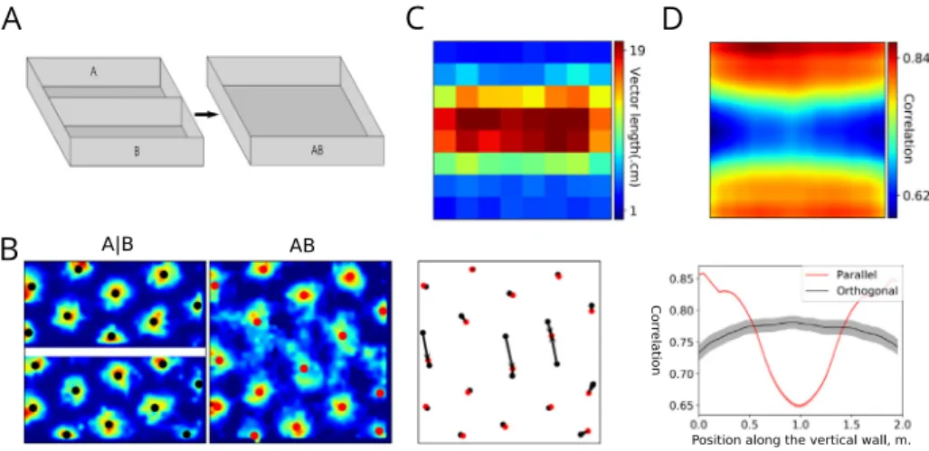
0). In the ‘dark’ condition, the model was run with visual cues turned off (i.e., uniform gray images were presented as visual input). Next, the trained model was run to cross the environment from left to right in the ‘light‘ and ‘dark‘ conditions as before, but with the speed gain in the grid cell populations modulated as described in the Results.

Fig. 4. Simulation of the merged-room experiment of Wernle et al. (2018). A. The training environment with two separate rooms, referred to as room ‘A|B’, and the testing environment, referred to as merged room ‘AB’. B. Firing fields of an example grid cell in the training (left) and testing (middle) environments, as well as firing-field displacement vectors calculated in the testing environment (right). C. A color map of mean vector lengths. D. Top plot: A color map representing the mean sliding correlation over all grid cells. Bottom plot: the correlation profiles at the center of the environment along two cardinal directions.

3.2. Simulation 2

In the original experiment (Wernle et al.,2018), the rats were trained in rooms A and B alternately for several days (seeFig. 4A for a schematic representation of the experimental environment). After that, the partition wall was removed and rats explored the merged room during a 45 min trial. Up to 9 such trials were performed daily in different animals. The simulation described below was designed to mimic this experimental protocol.

Training. The model was trained separately in room A and then

in room B for 30 min, which was sufficient to learn stable grid and place fields. Synaptic weights were then fixed to the learned values.

Testing. In the main experiment, simulated neural activities were

recorded while the model rat randomly explored the merged room for 1 h, with

α =

0

.

04. Two additional experiments were then performed. First, to test the influence of synaptic plasticity on the results of the main experiment, synaptic weights were updated as during training while the model rat additionally ex-plored the merged room for 1h. Second, to test the influence of the strength of the feedback loop, the model rat was run in the merged room for additional 20 one-hour trials. The value of

α

was decreased linearly from 0.04 to 0.005 across trials.

Sliding correlation. The sliding correlation heat maps for

grid-cell firing patterns were calculated as described inWernle et al. (2018). The size of the sliding correlation window was defined based on the grid spacing of the cell. The window moved from the top left to the bottom right corner in the grid field maps of the environment A

|

B (i.e. before the wall removal) and AB (i.e. after the wall removal). At each window location, the portion of the grid maps in the environments A

|

B and AB, outlined by the sliding window, were correlated with each other.

Displacement vector analysis. Displacement vectors were

calcu-lated as described inWernle et al.(2018). To obtain a displace-ment vector for one grid cell, the experidisplace-mental environdisplace-ment was divided into 4

×

4 blocks (50

×

50 cm each). In each block, the vector corresponding to the shift of grid fields in the environment AB relative to that in the environment A

|

B was calculated. The vectors were sorted into the corresponding blocks based on the grid field location in the training environment and the mean over all vectors was computed. To analyze displacement vector lengths, the environment was divided into 8

×

8 bins. The vec-tors were then sorted into the corresponding bins based on the

original grid field location in the training environment, and the mean vector length was computed.

3.3. Simulation 3

In the original experiment (Carpenter et al.,2015), rats foraged for food pellets during up to 20 daily experimental sessions in the experimental environment schematically shown inFig. 7A. Each session consisted of 2 trials, 40 min each. The two trials were identical, and were only needed to check for uncontrolled local cues possibly used by rats to identify the two compartments. At the beginning of each trial the rat was placed in the corridor between the two compartments facing the north wall and freely explored the environment. The simulation described below was designed to mimic this experimental protocol.

Training. During training, the model was placed in the center of

the corridor and then explored the complete environment quasi-randomly for 1 h. This learning period approximately represents a single training session of the original experiment. Eight such training sessions were performed, such that the strength of the feedback loop

α

decreased from 0.04 (first session) to 0.005 (last session) with step 0.005.

Testing. After each training session, the weights were fixed and

neural activity was recorded as the model rat explored the envi-ronment for 1 h.

Global and local fits. The firing rate maps of modeled grid cells

were fit with ideal local and global grid patterns using the proce-dure described inCarpenter et al.(2015). First, grid spacing was identified by correlating the firing pattern with 30 ideal firing grids. Each ideal grid pattern is a product of three cosine gratings

f (

−

→

x )

=

A

[

1

+

cos(

−

→

k 1(

−

→

x

+

−

→

c ))

] [

1

+

cos(

−

→

k 2(

−

→

x

+

−

→

c ))

]

×

×

[

1

+

cos(

−

→

k3(

−

→

x

+

−

→

c ))

]

with peak firing rate A, wave vectors

−

→

k1,

−

→

k2 and

−

→

k3 and

phase offsets

−

→

c

=

(cx

,

cy). The wave vectors are defined as

−

→

k

=

(2_λπcos(

ϕ

)

,

2_λπsin(

ϕ

)), where

λ =

√

3

2 G is the grating

wave length, G is the grid spacing and

ϕ

is the grid orientation. The 30 ideal grid patterns were created with grid spacing evenly distributed between 30 and 170 cm. Since the grid orientation in the model is set to 7.5◦

,

ϕ

in the three wave vectors is equal to 7.5◦

, 127.5◦

and 247.5◦

T. Li, A. Arleo and D. Sheynikhovich / Neural Networks 121 (2020) 37–51 43

were computed between the recorded firing rate map and the ideal grid patterns over a range of spatial phase offsets. The grid spacing of the recorded firing pattern is then set to that of the ideal grid pattern with the highest correlation. Second, local and global fits with the identified grid spacing were computed for the recorded firing rate map. The local fit was performed using two grid patterns (one per room) with the same phase offset. The global fit was performed using only one grid pattern with continuous phase across the two rooms. The Pearson product-moment correlation between the recorded firing rate map and the local and global grid patterns was computed over a range of phase offsets. The highest correlation with the local and global models was identified as the value of local and global fits, respectively.

4. Results

Since the early experiments testing the influence of visual and self-motion cues on place cell activity, it was clear that different subsets of place cells are controlled by these cues to different degrees, with some cells being controlled exclusively by one type of cue (Aronov & Tank,2014;Chen et al.,2013;Fattahi et al.,2018;Markus et al.,1994). In the model we conceptualized these differences in VPC, MPC and CPC neural populations, rep-resenting purely vision-dependent, motion-dependent and mul-tisensory place cells. Thus, after the model has learned place fields by moving quasi-randomly around a virtual rectangular box (Fig. 2A), VPCs had fields only in a ‘light’ condition, i.e. in the presence of visual cues (Fig. 2B, top row). This was true even if motion-based cues were absent, as in a passive transport through a virtual maze (Chen et al.,2013). Conceptually, these cells rep-resent the ability of hippocampal circuits to form self-organized representations of location even in the absence of grid-cell input from the mEC (Brandon et al.,2014;Hales et al.,2014;Schlesiger et al.,2018). In contrast, MPCs had place fields both in the light and dark conditions, but not during passive translation (Fig. 2B, middle row). Finally, CPCs were active in all the three conditions since they combine both types of input (Fig. 2B, bottom row).

In contrast to VPCs that are completely independent of self-motion cues and encode stable visual features of the surrounding environment, MPCs and CPCs are influenced by both visual and self-motion input, by virtue of their loop-like interactions through the grid cells. To assess the relative influence of vision and self-motion on the activity of these cells in a situation of sensory conflict, we decreased the gain of self-motion input to grid-cells while the model animal crossed the environment from left to right (Fig. 2C). This decrease in gain was applied only to the horizontal component of motion, i.e. the horizontal component of the self-motion velocity vector was set to 3

/

4 of the baseline value. Such a modification is similar to a change in the gain of translation from real-to-virtual movement in a virtual corri-dor (Chen et al.,2013), but implemented in a two-dimensional environment instead of a linear track. The change in gain resulted in a forward-shift of receptive fields of MPCs and CPCs relative to their position in baseline conditions and the size of the shift was smaller than what would be predicted from purely self-motion integration (Fig. 2E,F), expressing the correction of self-motion position code by visual cues.

To illustrate the loop dynamics in this simple example, con-sider the case when the model animal crossed the middle line of the environment moving from left to right (Fig. 2D). The inte-gration of pure self-motion input over time provides an estimate of the current position that is behind the actual position due to the decrease in speed gain. As a result, the place field of a purely self-motion dependent cell should shift ahead of the animal by an amount proportional to the gain factor (shown red dashed line in Fig. 2E,F). However, when visual cues are available, the VPC

population activity encodes the visual position estimate that is in independent of gain changes. As a result of the dynamic loop-like interaction, the VPC activity induces a forward shift of the activity packet in the grid-cell populations towards the visually identified location, and the size of this shift is controlled by the parameter

α

. Grid cells would similarly affect the MPCs, and then CPCs, closing the loop. Therefore, in the presence of conflicting cues, place fields shifted to an intermediate position between the self-motion and visual estimates, as shown by the distributions of place-field centroids in the MPC and CPC populations (Fig. 2E,F). A similar ef-fect of conflicting cues on place fields was experimentally studied by Gothard, Skaggs, and McNaughton (1996) and subsequently simulated in several computational models (Byrne et al., 2007; Samsonovich & McNaughton,1997;Sheynikhovich et al.,2009). However, in the present model the parameter controlling the interaction between the visual and self-motion cues is cast in terms of the strength of the entorhinal–hippocampal loop.

To illustrate the same multisensory integration mechanism on the level of grid cells, we conducted another simulation in which the horizontal velocity gain was only transiently decreased when the model animal crossed a specific portion of the environment (Fig. 3A). In this case of a transient cue conflict, grid patterns were locally deformed in that firing fields near the zone of decreased gain shifted forward relative to control conditions, reflecting the sensory conflict (Fig. 3B). Near the borders of the environment, where the speed input was identical to the baseline conditions, grid pattern remained stable. The same effect on the level of the whole population of grid cells was quantified by the analysis of displacement vectors (Fig. 3C) and by sliding correlation maps (Fig. 3D, see Section3.2for details of this analysis). These results suggest that local modifications of grid patterns can be induced by conflicting sensory representations, similarly to what has been observed in a recent experiment by Wernle et al. (2018). As mentioned in the Introduction, these observations are at odds with results of an earlier experiment (Carpenter et al., 2015) that studied adaptation of grid-cell patterns during construction of a spatial representation in an environment consisting in two identical rooms connected by a corridor. In the following sections we present simulations of the two experiments in an attempt to explain the conflict between them and to understand neu-ral mechanisms responsible for apparently different patterns of grid-cell adaptation in the two experiments.

4.1. Simulation of the merged-room experiment

Wernle et al. (2018) studied the integration between visual and self-motion cues by recording grid cells in two adjacent rect-angular compartments initially separated by a wall (seeFig. 4A). The two compartments were located inside a larger environment equipped with distal visual cues. The wall was subsequently removed and grid cells were recorded while the rat foraged in the merged room. The authors observed that at locations far from the removed wall grid cells conserved their firing patterns, while at locations near those previously occupied by the wall grid fields shifted so as to form a continuous quasi-hexagonal pattern (Wernle et al.,2018).

Simulation results from the previous section suggest that the observed local deformation of the grid pattern can result from the local visual deformation caused by wall removal. To verify that our model can reproduce these results, we recorded activities of simulated grid cells and place cells in experimental condi-tions similar to those in Wernle et al. (see Section 3.2). More specifically, in the training phase the model learned place fields separately in two virtual rooms A and B (Fig. 4A) located inside a bigger room with distal visual cues (not shown), such that learned representations of the two rooms were different after the

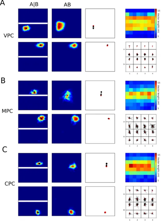
Fig. 5. Place fields in the merged-room experiment. A. Left: receptive fields of two VPCs in the training and testing environments, either close to the removed wall (top) or distal from it (bottom). Middle: displacement vectors of the cells on the left. Right: color map of displacement vector lengths for all cells (top) and all displacement vectors with their mean direction shown in red (right). B,C. Receptive fields and displacement vectors for MPCs (B) and CPCs (C). Refer to A for details.

initial exploration. In the testing phase, the wall was removed, the synaptic weights were fixed and neural activity was recorded while the model rate explored the merged room. We observed that after wall removal, grid fields near distant walls remained at the same location as during training, while those near the former wall location shifted towards it (Fig. 4B), as in the experiment. The same phenomenon on the level of the whole population was quantified by the analysis of displacement vectors (Fig. 4C) and by sliding correlation analysis (Fig. 4D).

Thus, the low-correlation band near the location of the re-moved wall was induced in the model by changes in visual input in the merged environment, which affected place coding via VPC activities. Local visual features at the locations distant from the removed wall were similar in the corresponding locations of the original environments A and B, since visual patterns formed by the closest walls and extramaze cues remained largely unchanged

after the central wall removal. Therefore, VPCs activities at these locations during testing were very similar to those during training (Fig. 5A), leading to the same grid pattern at these locations. However, at the locations close to the removed wall, the com-bined effect of stable distal cues and modified proximal wall cues resulted in an extension of VPC receptive fields over the previous location of the removed wall. Such changes in visual receptive fields induced local corrections of grid cell activity by shifting grid-cell activity packets towards the center, resulting in local deformations of grid-cell firing patterns similar to those observed during gain modification experiments. These deformations in turn affected place fields of MPCs and CPCs, by shifting place fields of the cells near the removed wall towards it (Fig. 5B,C). The results suggest that local deformations of grid fields can be explained by the same correction mechanism as the one studied in the previous section, but in which local sensory conflict is induced

T. Li, A. Arleo and D. Sheynikhovich / Neural Networks 121 (2020) 37–51 45

by changes in the visual input instead of changes in self-motion gain.

Two principal neural processes affect the formation of spa-tial representation in our model: while the acquisition of new spatial representations crucially depends on synaptic plasticity, the dynamic interaction between visual and self-motion cues is mediated by neuronal dynamics. We therefore tested the con-tribution of these two processes to the observed results. The influence of plasticity was assessed by letting the model learn during testing in the merged room, while that of neuronal dy-namics was tested by progressively decreasing the strength of the loop (i.e. decreasing the control of vision over self-motion cues) in the absence of synaptic plasticity. The results of these manipulations can be summarized as follows. First, when learning was allowed during testing and the testing trial in the merged room was sufficiently long, the particular correlation pattern (see Fig. 4C,D) was broken and a new representation was formed as a result of learning (Fig. 6A–C), unlike what was observed by Wernle et al. In particular, the newly formed global pattern was aligned with only one of the walls, resembling the results of Carpenter et al. (2015) addressed in the following section. Moreover, learning of the new representation was faster when the control of visual cues (controlled by

α

) was low (not shown), since slower dynamics favors the learning of new connections between self-motion-based and visual representations. Second, the decrease of

α

across separate sessions (with plasticity turned off) resulted in widening of the low correlation band (Fig. 6D). This modification of the correlation pattern is explained by the fact that under a weak control of place fields by vision, it takes longer for the visual cues to correct self-motion.

4.2. Simulation of the double-room experiment

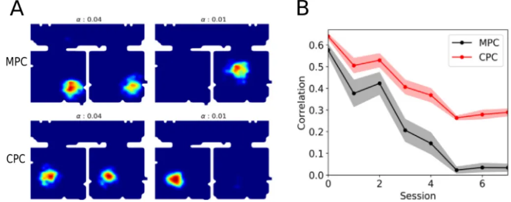
In the experiment ofCarpenter et al. (2015), grid cells were recorded in rats during foraging in an experimental environment consisting of two rectangular rooms (A and B) connected by a corridor (Fig. 7A, see alsoCarpenter et al.,2015). The two rooms were rendered as similar as possible in their visual appearance in order to favor visual aliasing. The rats were released in the cor-ridor and explored the whole environment for 80 min across up to 20 daily sessions. If local visual cues are the only determinants of grid cell activity, grid cells were expected to express identical hexagonal firing patterns in the two rooms, reflecting the same visual appearance of the rooms. However, since the animal is free to move between the rooms, self-motion cues can be used to spatially disambiguate them. Thus, if self-motion cues contribute to grid-cell firing, grid cells were in contrast expected to form distinct firing patterns in the two rooms. The results of this experiment revealed that both external and internal cues influ-ence neuronal activity, but in a temporally-organized fashion. In particular, grid cells had similar firing patterns in the two rooms during early exploration sessions, suggesting that local visual cues of the two rooms initially had a strong influence on grid-cell activities. As the number of sessions increased however, grid cells progressively formed a global hexagonal pattern extending over the whole environment suggesting a progressive contribution of self-motion cues. One consequence of the creation of the global representation was that local firing patterns in the two rooms progressively became more and more dissimilar despite the fact that visual cues remained the same. This can be interpreted as a progressive loss of control of local visual cues over grid-cell activities. These results are thus in conflict with the data from the merged-room experiment by Wernle et al. considered earlier, since in that experiment local visual cues near the distant walls kept their control of nearby grid fields for up to 9 consecutive sessions.

What could be the reason for the differences in learned grid-cell representations in the two experiments? Suppose that, in the conditions of the double-room paradigm, the rat first enters room A, such that initial associations between self-motion and visual cues are established in that room. The key question is whether or not a new representation for the subsequently entered room B will be formed, despite its identical visual appearance with room A (note that in the following we refer to any initially experienced room as room A, independently on which actual room was visited first in the simulations). Results of the previous section suggest that a weaker control of visual cues combined with synaptic plasticity leads to the formation of such a new representation. To verify this hypothesis, we ran our model in the conditions of Carpenter et al. experiment (see Section 3.3), and we pro-gressively (i.e. session by session) decreased the strength of the hippocampal-entorhinal feedback loop (without disabling synap-tic plassynap-ticity). As the feedback strength controls the influence of visual input in our model, we expected that this procedure will result in the construction of a global representation on the level of grid cells when the strength of the loop is sufficiently low. This was indeed the case as the global fit was high when the loop strength was set to low values (small

α

), and, conversely, the local fit was high for a strong loop (Fig. 7B,C, both of these measures were calculated in the same way as in the study by Carpenter et al. 2015, see Section3.3).

The local representation in early sessions is a consequence of the fact that representation of only one of the rooms is learned, so that once the model rat enters the second room, grid-cells activities are quickly reset by vision to the representation of the first (or, in terms of Skaggs and McNaughton (1998), the representation of room A is ‘‘instantiated’’ upon the entry to the room B). In this case both MPCs and CPCs had identical firing fields in the two rooms (Fig. 8A). This was quantified in the model by computing the spatial correlation between place fields of each cell in the two rooms (correlation of 1 corresponds to identical place fields). On the level of the whole population, the mean place-field correlation is high for a strong feedback loop (early sessions, large

α

,Fig. 8B). The transition to a global representation in later sessions results from newly formed synaptic associations between MPCs in CA3 (that are under a strong influence of self-motion input from grid cells), and CPCs in CA1 that are driven by vision. Synaptic plasticity at these connections is favored by a decreased hippocampal input to the EC, leading to a stronger reliance on self motion. The development of such a new repre-sentation is reflected in lower place-field correlation on the level of MPCs and CPCs (late sessions, small

α

,Fig. 8B). Note that purely vision-driven VPCs always have identical place fields in the two environments (not shown).

To summarize, the results of both the merged-room experi-ment of Wernle et al.(2018) and the double-room experiment of Carpenter et al.(2015) can be explained by the same model under two conditions: First, the hippocampal control over mEC grid cells progressively decreases in a familiar environment in the course of daily sessions (this requirement is crucial to re-produce the result of the second experiment, but, according to our simulations, has only a weak effect in the first); Second, synaptic plasticity is weak or inhibited when rats are placed into the merged room after learning in room A and B, but not when the rats are exposed to a stable double-room environment. What could be the reason for the inhibition of learning in the merged-room, as opposed to the double-room experiment? Analysis of our model offers the following possible explanation: In early ses-sions of the double-room experiment, a large mismatch between visual (i.e. encoded in VPC activities) and self-motion (encoded by MPC activities) input occurs at the moment of entry to, or exit from, the room B, since the population activity of VPSs ‘‘jumps’’

Fig. 6. Influence of plasticity and dynamics on grid patterns in the merged-room experiment. A,B. Displacement vectors (top) and corresponding sliding correlation maps (bottom) of two example grid cells after learning in the merged room. C. Averaged over many grid cells, sliding correlation maps can result in two different mean correlation patterns. D. Mean correlation along the direction perpendicular to the removed wall for different values of the strengthα.

Fig. 7. Simulation of the double-room experiment of Carpenter et al. 2015. A. Top view of the experimental environment with two visually identical rooms (A and

B). B. Population estimates of the local fit (red) and global fit (black) as a function of session number (see C and D for examples). The value of parameterαdecreased from 0.04 to 0.005 across sessions. C,D. Examples of firing rate maps of 4 different grid cells (rows) with superimposed ideal grid patterns according to the highest local (left column) or global (right column) fit. In each row the same firing map is shown twice. In early sessions (C) identical ideal grid patterns in the two rooms fit the data better than a single global hexagonal pattern: local fit is higher than the global fit. In late sessions (D) the reverse is true. The local and global fits were assessed from grid cell firing patterns in the rooms only (not in the corridor). (For interpretation of the references to color in this figure legend, the reader is referred to the web version of this article.)

to reflect the room A cues or the corridor cues, respectively. This jump of population activity can be quantified by the drop in correlation between the projections of VPCs and MPCs in CA3 onto the CPCs in CA1 near the room doors (Fig. 9A). In contrast, the mismatch is smaller for the merged-room experiment, since the visual and self-motion cues near the removed wall code for similar spatial positions (Fig. 9B). Therefore, it is possible that learning across sessions is regulated by the size of the mismatch between visual and self-motion cues. Note that statistical char-acterization of the mismatch in Fig. 9required averaging over many experimental runs and even in our idealized model cannot be reliably detected online. This could be a possible reason why building of a global environment representation in Carpenter et al. experiment takes many days. We thus propose that CA1 area

or, more likely, its output structures implement a mismatch de-tection process that can regulate hippocampal synaptic plasticity on the time scale of days.

5. Discussion

The presented model is based on two main assumptions: that of a loop-like dynamics in the entorhinal–hippocampal net-work, and that of an independent visual place-cell representation formed on the basis of hippocampal inputs other than grid cells. Place cells in CA1 receive inputs from spatial (including grid cells) and non-spatial entorhinal cells (Zhang et al.,2013), either via a direct projection from mEC or via an indirect pathway through the DG and CA3. Lesion experiments have shown that either of

T. Li, A. Arleo and D. Sheynikhovich / Neural Networks 121 (2020) 37–51 47

Fig. 8. Evolution of place fields in the double room experiment. A. An example of MPC (top) and CPCs (bottom) place field during early learning sessions (left column, highα) and late sessions (right column, lowα). In early sessions a majority of place cells have similar place fields in the two rooms, whereas in late sessions a majority of place cells have a place field only in one of the rooms. B. Spatial correlation between place fields of a cell in the two rooms, averaged over all place cells, as a function of session number (or, equivalently, as a function of decreasing value ofα.

Fig. 9. Mismatch between the visual and self-motion representations in the double-room (A) and merged-room (B) experiments. The colors denote the correlation between VPCs and MPCs projections onto the CPC population.

these pathways can support location-sensitive activity of the hip-pocampal CA1 neurons (Brun et al.,2008,2002). Moreover, even after massive EC lesions CA1 cells retained their spatial selectivity of Van Cauter, Poucet, and Save (2008), suggesting that such selectivity can result from a large variety of afferent inputs to this structure. Place cells in CA1 project back to the entorhinal cortex both directly and via subiculum (Kloosterman, van Haeften, Wit-ter, & Lopes da Silva,2003;Naber, Lopes da Silva, & Witter,2001; Slomianka et al.,2011) and hippocampal input is necessary for grid cell activity (Bonnevie et al.,2013), supporting the loop-like structure of entorhinal–hippocampal interactions (Iijima et al., 1996;Mizuseki, Sirota, Pastalkova, & Buzsáki,2009).

That a subset of hippocampal place cells can form spatial rep-resentations independently from grid cells is supported by a sub-stantial amount of evidence (Poucet et al.,2013). In particular, in rat pups place cells are present before the emergence of the grid cell network (Muessig et al.,2015), whereas in adult rats a disrup-tion of grid cell activity does not prevent the appearance of place cells in novel environments (Brandon et al.,2014). These grid-cell independent place codes retain all principal properties of a self-organized representation in control animals: they can be learned in new environments, they are stable over time, and independent representations are established in different rooms (Rueckemann et al.,2016;Schlesiger et al.,2018). These data suggest the ex-istence of two parallel and overlapping input streams that give rise to hippocampal place sensitivity: the first one integrating spatial inputs from grid cells in the dorsal mEC, likely represent-ing self-motion-based spatial signals (McNaughton et al.,2006); the second one integrating other sensory information to form a grid-cell independent spatial representation in a self-organized manner (Poucet et al., 2015). The differential reliance of place cells on these principal input streams is most clearly manifested

in neural responses of these cells to sensory manipulations in vir-tual linear track experiments (Chen et al.,2013): during passive movement through the track (i.e. with only visual cues available) 25% of cells kept their firing fields unchanged relative to a control condition with both types of cues present; during locomotion in the absence of visual cues (i.e. with only self-motion cues avail-able) 20% of cells did not change their firing patterns; the activity of the rest of CA1 cells was modified to various degrees by cue manipulations (see alsoHaas, Henke, Leibold, & Thurley,2019). Moreover, recent evidence suggests that CA1 cells responsive to visual and self-motion input are anatomically separated: place cells more responsive to self-motion cues are located predomi-nantly in superficial layers of CA1, while those more responsive to visual cues are found in deep layers (Fattahi et al.,2018;Mizuseki, Diba, Pastalkova, & Buzsáki,2011). It was also recently shown that CA1 cells in deep and superficial layers receive stronger excitation from mEC and lEC, respectively, with the amount of excitation being also dependent on the position of the neurons along the longitudinal hippocampal axis (Masurkar et al.,2017). These data further support the existence of functionally different subsets of place cells in CA1, that can either be inherited from similarly segregated cells in CA3 or to be formed directly from non-grid EC inputs to CA1.

Our model is constructed to reflect the above data in a sim-plified way. While the neural basis for the aforementioned grid-cell-independent code is not clear, we conceptualized it by a population of VPCs, which learn subsets of visual features corre-sponding to a particular location using simple competitive learn-ing scheme. Similarly to experimental data described above, VPCs form a stable and independent code for different environments as long as visual cues in these environments are stable. It is likely that such a code is formed inside the hippocampus itself

based on the inputs either from lEC (Schlesiger et al., 2018) or ventral mEC (Poucet et al.,2013) possibly together with in-puts from other structures (Van Cauter et al., 2008), since no location-sensitive code has been observed directly upstream of the hippocampus (Mao, Kandler, McNaughton, & Bonin, 2017). While in its current version our model assumes that VPCs are learned in CA3 and transmitted to CA1, the model can be modi-fied to implement competitive learning in CA1 directly on visual inputs from lEC, bypassing CA3 (Brun et al.,2002). Similarly to a number of attractor-network models of grid-cell activity ( Bon-nevie et al., 2013; Burak & Fiete, 2009; Fuhs, 2006; Guanella et al.,2007;McNaughton et al.,2006;Sheynikhovich et al.,2009), our model of self-motion-driven activity in GC-MPC populations relies on the assumptions that (i) the position of the animal in an environment is represented by the position of the activity packet (i.e., an attractor state of network dynamics) on a 2D neural sheet corresponding to a grid-cell population; and that (ii) the activity packet is shifted to precisely integrate the animal’s velocity. As long as these assumptions hold, our modeling results are independent of the exact neural mechanisms realizing the attractor dynamics and velocity-based shifts of the attractor state (provided that the hippocampal input can influence the attractor state according to Eqs.(1)–(2)).

The main contribution of the present model is the proposal that integration of visual and self-motion representations occurs in the EC and is regulated via feedback projections from the CA1. This is in contrast to a long-standing idea that multisen-sory integration is performed by the attractor network residing in CA3 (McNaughton et al.,1996; Samsonovich & McNaughton, 1997). Our model thus resolves two outstanding issues related to this earlier proposal. The first issue is the existence of separate self-motion-dependent and vision-dependent subsets of cells in CA1/CA3 mentioned above (Chen et al., 2013; Chen, Lu, King, Cacucci, & Burgess,2019;Fattahi et al.,2018;Haas et al.,2019). If CA3 performed the integration of the two representations as the earlier model suggests, why would they still persist in the downstream CA1? In our model, the existence of the two rep-resentations in CA1 are essential for the model to work, since their combined input to the EC is required for multisensory integration. The second issue is the mutual interaction between external/sensory and self-motion-based representations. In ear-lier models cognitive mapping was essentially performed by a ‘‘path integrator’’ (that is now thought to reside in the grid-cell network) and the role of visual input was only to occasionally reset it and to prevent error accumulation. As discussed above, it is now clear that external sensory inputs can self-organize into a stable and persistent representation and that neural mechanisms supporting such a representation appear earlier during develop-ment than the putative path integration system. It is thus possible that the two representations exist in parallel and interact with each other. Here we propose how such an interaction can be performed by the entorhinal–hippocampal processing loop. We believe that studies of grid cells and place cells in environments with visually similar compartments provide an important line of experimental evidence as to the modes of interactions be-tween the two representations, since in these studies the two types of information are put in direct conflict. Previous models that addressed mutual relations between place cells and grid cells (Guanella et al.,2007; Rennó-Costa & Tort, 2017) focused on other aspects of such relations. While our model postulates the important role of hippocampal CA1 representation in the correction of cumulative error at the level of grid cells, it does not exclude the involvement of other possible mechanisms of error correction. For example, it has been recently proposed that border cells, experimentally observed in mEC, correct grid-cell activity near environmental boundaries (Hardcastle, Ganguli, & Giocomo,

2015). It is not clear how such a boundary-related processing can affect grid cells far from boundaries, for example in the conditions of experimental studies simulated in the present work. In addi-tion, it is not clear whether the boundary-based error correction occurs independently of the hippocampal input, as proposed by Hardcastle et al. or via the hippocampal processing loop, in which case it will be a particular case of the model proposed here. The relative contribution of different mechanisms, if they exist, will potentially be determined by the features of the environment, such as the presence of distal cues, objects and boundaries.

An important parameter of our model is the strength

α

of the feedback projection from CA1 to EC, reflecting the efficacy of neural information transmission between the two areas ( Bon-nevie et al., 2013; Colgin et al., 2009). The progressive con-struction of a global representation in our simulation of the double-room experiment required a progressive decrease in the value of this parameter. By slowing down the dynamical cor-rection of motion-based entorhinal-CA3 representation by vision, it allowed synaptic plasticity in afferent CA1 synapses to form new associations between a visual representation of the rooms (encoded in the VPC activity) and the motion-based represen-tation, and hence to disambiguate the two rooms. Ultimately then, whether a global representation was learned or not is determined by the relative time scales of two processes: (i) dy-namical correction of EC attractor states and corresponding CA3 representations by external visual cues and (ii) synaptic plas-ticity at afferent CA1 synapses. The interplay between the two processes can in principle be governed by several neuronal mech-anisms, including neuromodulatory influences on plasticity and neural dynamics (Hasselmo, Schnell, & Barkai,1995) and/or on oscillation coherence (Colgin et al., 2009). While in our simu-lations

α

was manually decreased across sessions, the model could be extended to automatically adjust its value. One possi-bility would be to link the value

α

to novelty processing: upon initial exposure to an environment the novelty signal is high (potentially reflecting the absence of learned connections be-tween motion-based and vision-based representations), while it should progressively decrease as these connections are learned and motion-based CA3 representation takes precedence over ex-ternal sensory inputs (Hasselmo et al.,1995). Another possibility is to consider the hippocampal loop processing as a network to implementing statistical inference and prediction (Bousquet, Bal-akrishnan, & Honavar,1997;Penny, Zeidman, & Burgess,2013): in a novel environment, prediction about future incoming sensory inputs is poor (high prediction error); as learning progresses this error decreases reflecting a better statistical model of the envi-ronment. These considerations suggest that a global representa-tion must eventually arise after a sufficiently long exposure to an environment. This was not however the case in the merged-room experiment. Indeed, under the hypothesis that grid cells express hexagonal firing patterns as a consequence of attractor dynamics with circular weight matrices (McNaughton et al., 2006), the local translocation of grid fields at the center of the merged environment must result from a dynamic correction mechanisms, since synaptic plasticity between place-cell and grid-cell net-works would necessarily lead to the emergence of a coherent (global) grid-cell representation. One possible explanation for this discrepancy is that the testing period in the merged room (up to 9 daily sessions) was not long enough, as rats in the double-room experiment expressed clearly global grid patterns after at least 10 testing sessions (Carpenter et al., 2015). Another possibility suggested by the analysis of the model is that the learning process is also regulated by the size of the mismatch between visual and self-motion-based representations.

A number of experiments studied place fields dynamics in environments consisting of two or more visually identical com-partments (Fuhs, VanRhoads, Casale, McNaughton, & Touretzky,