Control allocation for the next generation of entry vehicles

(1)

Control Allocation for the Next Generation of Entry Vehicles

by

Richard H. Shertzer B.S. Engineering Mechanics United States Air Force Academy, 1999

SUBMITTED TO THE DEPARTMENT OF AERONAUTICS AND ASTRONAUTICS IN PARTIAL FULFILLMENT OF THE REQUIREMENTS FOR THE DEGREE OF

MASTER OF SCIENCE IN AERONAUTICS AND ASTRONAUTICS

AT THE

MASSACHUSETTS INSTITUTE OF TECHNOLOGY

June 2001

The author hereby grants to MIT permission to reproduce and to distribute publicly paper and electronic copies of this thesis document in whole or in part.

Signature of Author

Department of Aeronautics and Astronautics May 11, 2001

Approved by

Douglas J. Zimpfer Charles Stark Draper Laboratory Technical Supervisor

Certified by_

Rudrapatna V. Ramnath Senior Lecturer, Department of Aeronautics and Astronautics Thesis Advisor

Accepted by

Wallace E. Vander Velde

MASSACHUSETS INSTITUTE Professor of Aeronautics and Astronautics

OF TECHNOLOGY _{Chair, Committee on Graduate Students}

SEP 112001

LIBRARIES

(2)

(3)

Control Allocation for the Next Generation of Entry Vehicles

by

Richard H. Shertzer

Submitted to the Department of Aeronautics and Astronautics on May 11, 2001 in Partial Fulfillment of the

Requirements for the Degree of Master of Science in Aeronautics and Astronautics

Abstract

Control allocation is the process of assigning control responsibility amongst redundant actuators. A control allocation algorithm for an entry vehicle is presented that uses a linear program to optimally specify bounded aerosurface deflections and jet firings in

response to torque commands. Actuator preference is introduced via an objective

function to produce a unique solution when the system of linear equations is underdetermined. A multivariable control law is adopted to drive the control allocation algorithm and to track the desired state of the entry vehicle model. Open loop and closed loop tests are conducted to demonstrate dynamic objective calculation, blended aerosurface/jet capability, and efficient reconfiguration in the event of actuator failure. An approach is also presented to define the relationship between systematic errors in measured vehicle state and the actuator commands produced by the control allocation algorithm. Potential control allocation applications beyond the entry problem and other recommendations for further research are stated in the concluding remarks.

Technical Supervisor: Douglas J. Zimpfer

Title: Senior Member Technical Staff, C.S. Draper Laboratory, Inc.

Thesis Supervisor: Rudrapatna V. Ramnath

(4)

(5)

Acknowledgement

My greatest debt of gratitude goes to my wife, Amy, who has been loving and thoughtful

during two years of separation. Although she will miss the visits to Boston, neither of us will miss the good-byes. I also appreciate the support from both my family and hers during this research effort.

I would like to thank the Charles Stark Draper Laboratory for the opportunity to pursue

my graduate education at MIT with both technical support and financial means. I am indebted to my Draper supervisors, Doug Zimpfer, Pat Brown, Piero Miotto, and Gregg Barton for volumes of advice and assistance. Steve Kolitz and Steve Clark also offered their resources and experience regarding optimization techniques. I would also like to thank Jennifer Hamelin and Roberto Pileggi for their technical guidance during my first year at the Draper Laboratory.

I am also grateful to the faculty and staff at MIT's Department of Aeronautics and

Astronautics. Particular thanks go to my thesis advisor, Dr. Rudrapatna Ramnath, for his guidance and support.

Lastly, I would like to thank my friends for enlivening the MIT experience. Raja and Steve always made lunch an interesting time and the MIT weight room will never quite be same now that Raja has left his mark. Best of luck to Chris and Ted in the upcoming year. John J. and Rich are great housemates and I wish them luck as they enter pilot training. To all others with whom I've enjoyed intramural basketball, ski weekends,

sightseeing jaunts, and baseball games - thanks for the memories.

This thesis was prepared at The Charles Stark Draper Laboratory, Inc. under Internal Research & Development Project #13033.

Publication of this thesis does not constitute approval by Draper or the sponsoring agency of the findings or conclusions contained herein. It is published for the exchange and stimulation of ideas.

Richard H. Shertzer 2Lt, USAF

(6)

(7)

Table of Contents IN TR O D U C TIO N ... 15 1.1 THESIS O BJECTIVES ... 16 1.2 THESIS PREVIEW ... 16 EN TR Y C O N TR O L O V ER V IEW ... 19 2.1 SPACE SHUTTLE ... 19 2.2 CURRENT EFFORTS... 21 SY STEM A R C H IT E C TU R E ... 27 3.1 OVERVIEW ... 27

3.2 V EHICLE DESCRIPTION AND DYNAMICS... 28

3.3 TRAJECTORY GENERATION ... 34

3.4 GUIDANCE AND CONTROL...34

C O N TR O L A LL O C A TIO N ... 39

4.1 OVERVIEW ... 39

4.2 THE LINEAR PROGRAM ... 40

4.3 UPPER AND LOW ER BOUNDS... 51

4.4 OBJECTIVE FUNCTION COEFFICIENTS... 52

4.5 ACTUATOR CONTROL AUTHORITIES ... 55

4.6 PULSING LOGIC ... 58

4.7 OPEN LOOP TESTS: CONTROL ALLOCATION ISOLATION ... 59

C LO SED L O O P SIM U LA TIO N S ... 67

5.1 LOW ALTITUDE ENTRY SIMULATIONS... 68

5.2 HIGH ALTITUDE ENTRY SIMULATIONS... 73

5.3 ACTUATOR FAILURE SIMULATIONS... 81

5.4 COMPUTATIONAL EFFICIENCY ... 85

ACTIVITY VECTOR UNCERTAINTY...87

6.1 ANALYSIS M ETHOD ... 87

6.2 SAMPLE DATA ... 89

CONCLUSIONS AND RECOMMENDATIONS... 95

(8)

APPENDIX B: ADDITIONAL SIMULATION RESULTS ... 103

(9)

List of Figures

Figure 2-1. Shuttle-based Guidance and Control... 20

Figure 2-2. Shuttle-based Longitudinal Control ... 21

Figure 2-3. MIMO/Control Allocation Architecture ... 22

Figure 3-1. Sim ulation A rchitecture ... 27

Figure 3-2. Diagram of the X-34 [12]... 29

Figure 3-3. X-34 RCS Configuration ... 31

Figure 3-4. LQ-Servo with Integrators ... 35

Figure 4-1. Control Allocation Architecture... 39

Figure 4-2. Geometry of Example I ... 43

Figure 4-3. Geometry of Example I with Upper Bound on x ... 45

Figure 4-4. Geometry of Example 1 with Objective Function z =IxI + 4. -X2 ... . .. . . . . 46

Figure 4-5. Pitching Moment vs. Elevon Deflection ... 50

Figure 4-6. Example of crate Objective Coefficient Contribution ... 54

Figure 4-7. Open Loop Test #1: Commanded and Measured Torque ... 60

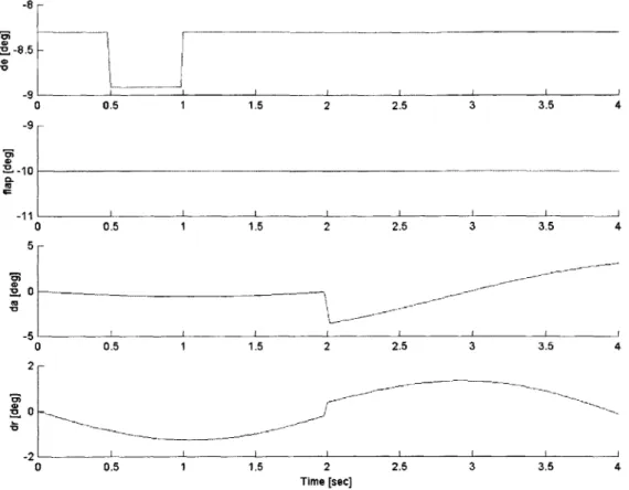
Figure 4-8. Open Loop Test #1: Actuators ... 61

Figure 4-9. Open Loop Test #2: No Objective Function ... 62

Figure 4-10. Open Loop Test #2: Objective Function Applied ... 62

Figure 4-11. O pen Loop Test #3... 64

Figure 5-1. Low Altitude Entry Simulation: Nominal Case (1 of 6)... 69

(10)

Figure 5-8. Low Altitude Entry Simulation: 60' Bank Turns (2 of 3) ... 72

Figure 5-10. High Altitude Entry Simulation: Pitch Maneuver / Low Elevon Cost...75

Figure 5-11. High Altitude Entry Simulation: Pitch Maneuver / Medium Elevon Cost...75

Figure 5-12. High Altitude Entry Simulation: Pitch Maneuver / High Elevon Cost...76

Figure 5-13. High Altitude Entry Simulation: Roll Maneuver (1 of 2)... 77

Figure 5-14. High Altitude Entry Simulation: Roll Maneuver (2 of 2)... 78

Figure 5-15. High Altitude Entry Simulation: RCS Only (1 of 3)... 79

Figure 5-18. Actuator Failure Simulation: Elevon Stuck at t = 20s (1 of 3)... 81

Figure 5-19. Actuator Failure Simulation: Elevon Stuck at t = 20s (2 of 3)...82

Figure 5-20. Actuator Failure Simulation: Elevon Stuck at t = 20s (3 of 3)... 82

Figure 5-21. Actuator Failure Simulation: No Rudder until t = 20s (1 of 3)... 83

Figure 5-22. Actuator Failure Simulation: No Rudder until t = 20s (2 of 3)... 84

Figure 5-23. Actuator Failure Simulation: No Rudder until t = 20s (3 of 3)... 84

Figure 6-1. Open Loop Path from Mcmd to Mmea, (1 of 3)... 87

Figure 6-2. Open Loop Path from Mcmd to Mmeas (2 of 3)... 88

Figure 6-3. Open Loop Path from Mcmld to Mm.eas (3 of 3)... 89

Figure 6-4. Example Data: K3 vs. Full Range of Mcmds / demds ... 90

Figure 6-5. Example Data: K3 vs. Reasonable Range of Memds / decmds ...--- ..-... 91

Figure 6-6. Example Data: K3 and Magnitude of Gain Uncertainty vs. % Error in Mach ... 92

Figure 8-1. Solution A lgorithm Overview ... 99

Figure 9-1. Low Altitude Entry Simulation: 60' Bank Turns (1 of 6) ... 103

(11)

Figure 9-7. Actuator Failure Simulation: Elevon Stuck at t = 20s (I of 6)... 106

Figure 9-8. Actuator Failure Simulation: Elevon Stuck at t = 20s (2 of 6)... 106

Figure 9-13. Actuator Failure Simulation: No Rudder until t = 20s (1 of 6)... 109

Figure 9-15. Actuator Failure Simulation: No Rudder until t = 20s (3 of 6)... 110

Figure 9-17. Actuator Failure Simulation: No Rudder until t = 20s (5 of 6)... 111

(12)

(13)

List of Tables

Table 3-1. Physical Characteristics of the X-34 [1 1]...29

Table 3-2. Entry Actuator Characteristics ... 30

Table 3-3. X-34 RCS Firing Patterns... 32

Table 3-4. Description of State Variables... 33

Table 3-5. LQ-Servo Variable Definitions ... 35

Table 4-1. Open Loop Simulation Parameters... 60

Table 5-1. High Altitude Simulation Parameters... 74

Table 5-2. Control Allocation Algorithm Iterations ... 85

Table 6-1. Example Data: Worst-Case Parameter and Gain Uncertainty... 92

(14)

(15)

1 INTRODUCTION

The next generation of aircraft and aerospace vehicles will require control laws that utilize

the full capability of available control effectors. This is necessary to meet safety and

operational cost requirements, but it is a task that becomes increasingly difficult as control actuators grow in both number and complexity. Traditional aircraft possess three basic

aerodynamic controls, one for each of the rotational degrees of freedom. Conversely,

modem tactical aircraft have unconventional control effectors, such as canards and thrust vectoring, which serve to complement or replace the standard assortment of aileron, elevator, and rudder. The one-to-one correspondence between rotational degrees of freedom and vehicle controls no longer exists with the addition of modem control effectors. Vehicles that possess this type of control redundancy present both unique design possibilities and potential

complications. One obvious benefit is that reconfiguration, necessary in the event of

individual actuator failures, is more easily achieved when a collection of redundant control effectors is present. Redundancy across many actuators saves both cost and weight because no longer are individual actuators burdened with excess levels of redundancy. Of course, designing control laws that take advantage of control redundancy can be a difficult task. In an effort to avoid complexity, many prospective control approaches compartmentalize tasks rather than directly command a complex arsenal of actuators. A controller, in the traditional sense, is still responsible for tracking, stability, and disturbance rejection, while a separate control allocation algorithm transforms generalized commands from the controller into actuator commands. This modular approach preserves simplicity by allowing command of controlled degrees of freedom rather than scheduling the concerted effort of many redundant actuators.

Control redundancy is not exclusively inherent to tactical aircraft with unconventional aerosurfaces and thrust vectoring. Any entry vehicle requires control redundancy during the transition from exo- to endo-atmospheric flight. At extreme altitudes, reaction control system (RCS) jets are used to stabilize the vehicle because aerosurfaces lack sufficient control authority. A gradual transition ensues as the aerosurfaces gain control authority and the RCS jets become ineffective. Future aerospace vehicles must be equipped to manage not

(16)

only the entry transition and subsequent atmospheric flight, but also powered ascent, the

control transition from atmospheric ascent to orbit, and on-orbit operations. These

procedures require a combination of traditional aircraft and spacecraft control effectors. To command this gamut of actuators, existing aerospace vehicles piece together different control strategies according to the current flight phase or transition. As aerospace vehicles expand the operational envelope, carrying with them a host of control effectors, piecemeal control algorithms become cumbersome and complicated. In order to move toward flexible and robust control approaches it is necessary to logically separate the tasks of control and

actuator assignment. A control allocation algorithm supplements a control law by

distributing control responsibility amongst the different families of currently available actuation devices.

1.1 THESIS OBJECTIVES

The objective of this research task is to develop a simple and physically intuitive control allocation algorithm for an entry vehicle. The algorithm will translate generalized control commands into RCS and aerosurface commands, applying feasible limits of the physical hardware as necessary. Reliable and efficient reconfiguration as the flight environment evolves or in the instance of actuator failure must be inherent to the design. In addition, the design should exhibit computational efficiency insofar as to not preclude eventual onboard implementation.

The aforementioned tasks coincide with the Draper Laboratory's ongoing development of

next-generation guidance and control algorithms. Advances in real-time trajectory

generation and abort technology will hasten the departure of sequential, gain-scheduled

control systems. As more robust control strategies are required, control allocation of

redundant actuators will become a necessary design element.

1.2 THESIS PREVIEW

The chapters in this thesis illustrate the development and evaluation of the control allocation algorithm. Chapter 2 describes the genesis and progression of control allocation techniques,

(17)

characterizing this research effort in the context of other approaches. As described above, control allocation is a single element in a complete flight control structure; Chapter 3 is an overview of the comprehensive model. Included in this chapter are descriptions of necessary simulation elements, such as a vehicle model and guidance and control algorithms. The details of the control allocation algorithm are revealed in Chapter 4. This chapter includes an academic discussion of the algorithm and practical issues surrounding application to entry flight. Open loop simulations isolating the control allocation algorithm are also presented in

Chapter 4. Closed loop simulations follow in Chapter 5. The first sections in Chapter 5

consider entry flight, highlighting the transition from exo- to endo-atmospheric flight. This control effector transition implies efficient revision of actuator assignment as the flight

environment evolves. The latter sections in Chapter 5 investigate less common

circumstances requiring actuator reconfiguration; the cases presented here involve actuator

failure. The final section in Chapter 5 briefly discusses the computational efficiency

exhibited by the algorithm throughout all simulations. Control allocation is a model-based algorithm, and Chapter 6 explores the relationship between errors in state feedback and modeling errors. Lastly, Chapter 7 discusses conclusions to be drawn from this work and recommendations for future research.

(18)

(19)

2 ENTRY CONTROL OVERVIEW

This chapter presents a brief evolution of entry control techniques and control allocation

methods. Control allocation algorithms were born when deficiencies surfaced in the

guidance and control algorithms that govern advanced aerospace vehicles. Because this thesis applies control allocation specifically to the entry problem, the heritage of advanced

aircraft guidance and control is ignored in favor of the Space Shuttle. Current demonstrators of entry and reusable launch technologies still apply the guidance and control algorithms developed for the Space Shuttle. Alternative designs have matured but none has replaced the original approach. Many of these alternative guidance and control algorithms employ some form of control allocation. The underlying problem in control allocation is to find a way to map generalized control requests into meaningful actuator commands. Currently, methods of solving the allocation problem fall into two groups: those that consider the geometry of the problem and those that do not.

2.1 SPACE SHUTTLE

The legacy of Space Shuttle entry guidance and control has survived to this day because it is a proven solution. Prescribed entry trajectories, heavily constrained by heating concerns, are executed by sequentially applied control strategies during descent. Entry trajectories consist of two basic parts: an initial high angle-of-attack portion intended to induce drag and lower the vehicle's energy state, and a low angle-of-attack segment for trajectory control [1]. The shift between these trajectory divisions incorporates an obvious angle-of-attack transition and a control effector transition. In general, RCS jets are treated as high altitude, low dynamic pressure controllers while aerosurfaces dominate the terminal flight phase where the air is thicker and the vehicle speeds are slower [2]. Particular attention is paid to the yaw channel during transition because the rudder is the last aerosurface to gain adequate control authority. This is true because the vehicle body effectively blocks airflow over the rudder at high angle-of-attack. Aileron and elevator could be used to control yaw while the rudder is ineffective, but then only two aerosurfaces are controlling three axes and control of each axis is no longer independent of the other axes. Because the need for blended control between the RCS jets

(20)

and aerosurfaces is evident, the entry digital autopilot (DAP) uses gain-scheduled control commands to aileron, elevator, and rudder while simultaneously applying a simplified phase-plane logic for supplemental RCS control [2]. The entry DAP philosophy treats the jets as low frequency control devices, sufficient to provide rate damping and attitude limiting, with

wide deadbands, particularly for pitch and roll. The assumption is made that the

aerosurfaces, high frequency control devices, will exert precise control within these deadbands.

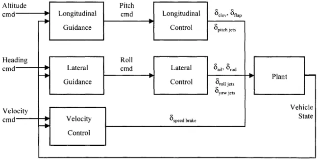
Figure 2-1 shows the basic architecture of the entry DAP. The principal characteristic is the separation of lateral and longitudinal dynamics, a shortcoming from a control perspective. If the vehicle rolls it loses lift and drops in altitude, however, the longitudinal controller does not respond to this maneuver until sensors detect altitude errors. The control loops must react to each other rather than work together to efficiently achieve common goals. Separating longitudinal and lateral dynamics ignores the coupling between axes that exists in a typical flight vehicle. Inertia and the influence of control surfaces cause such coupling.

Figure 2-1. Shuttle-based Guidance and Control

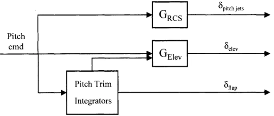
Figure 2-2 is a closer look into the longitudinal control block from above. The figure

(21)

algorithms. The presence of many single-input-single-output (SISO) loops greatly limits coupling of redundant actuators. The body flap, elevators, and pitch jets provide an example of such a limitation. These are redundant actuators during entry, but they are scheduled via

separate control loops with predetermined control gains. Because no cross-channel

communication exists, each loop operates without knowledge of what the other loops are

doing. Managing groups of actuators with independent control logic works well for

predefined trajectories. However, a Shuttle-based entry algorithm could give rise to reduced controllability in an instance of actuator saturation or failure. In these extreme cases the Shuttle-based algorithm must alter the specific allocation of physical controls, a process resulting in control inefficiency at the very least. The alternative is to schedule gains for all control redundancy/deficiency conditions. This is an undesirable design task, especially because these conditions will change appreciably during flight.

*

Gacs

pith jets

Pitch

cmd

G

lev

G

r Elev ee

Pitch Trim Sflap

Integrators

Figure 2-2. Shuttle-based Longitudinal Control

2.2 CURRENT EFFORTS

A multiple-input-multiple-output (MIMO) controller resolves many of the shortcomings evident in traditional SISO design. A multivariable approach considers the effects of all control inputs on all of the vehicle states. This allows the entire set of vehicle dynamics to be incorporated in a single design rather than separating dynamics and actuators into separate loops. Although MIMO designs offer the benefit of coupled dynamics, they tackle the subject of control allocation in essentially identical fashion as their SISO cousins: gain

(22)

scheduling to account for instances of actuator redundancy and failure. A design is more straightforward and equally effective if it separates the control and actuator allocation problems (Figure 2-3). This alleviates the need for actuator gains and permits the MIMO design to produce meaningful vehicle commands in response to vehicle state errors. Regardless of the control law, control allocation algorithms are valuable design elements. This is true because, in the presence of control redundancy or deficiency, it is both simpler and more robust to design for actuator selection using a dedicated control allocation design. The marriage of control allocation and a multivariable control law is not essential; any control law can be designed to produce generic rotational and/or translational commands. However, pairing a MIMO design and control allocation algorithm results in a flexible and robust flight control structure, precisely the characteristics required by the next generation of aerospace vehicles.

State Integrated Rotational &

References Translational cmds Conro P

-y GuidancePln _

Allocation

& Control

Vehicle State

Figure 2-3. MIMO/Control Allocation Architecture

2.2.1 The Control Allocation Problem

The constrained control allocation problem is as follows: derive physically meaningful actuator commands from generalized control commands. Three possible outcomes exist: 1) one unique solution, 2) many acceptable solutions, and 3) no solution. In the first case no control redundancy exists. This problem can be solved just as effectively by a controller directly commanding actuator deflections. In the second case there is control redundancy and some method of actuator prioritization must be established in order to distribute commands between redundant actuators. In the final case there is control deficiency. The

(23)

problem now becomes a prioritization between roll, pitch, and yaw because available actuators cannot simultaneously satisfy all control commands.

Initial control allocation efforts used pseudo-control or pseudo-inverse solutions to map

generalized controller commands to aerosurface commands [3]. Conventional

pseudo-control and pseudo-inverse techniques do not explicitly allow for actuator limits or designer preferences for specific effector usage. In order to realize these goals the control laws must be carefully tuned, much like the original Shuttle-based algorithm. Based on experience gained from these first attempts, designers chose to augment inverse and pseudo-control methods with objective functions. This methodology enforces actuator limits and

provides performance criteria through the objective function. At present, most control

allocation techniques rely on some form of objective optimization. However, a technique also exists that solves for the optimal allocation solution without using an objective function. This method will be described first, followed by approaches using objective optimization.

2.2.2 Geometric Approach

The geometric problem is developed in references [4-6]. Simply put, this method first

defines an attainable moment set based on all available physical control actuators and their limits. Torque commands, the generalized control command, represent a vector within this attainable moment set. One benefit of the geometric approach is the utilization of torque commands. Specifying physically meaningful control variables permits the designer to use intuition when tackling the control and control allocation problems. The set of actuators that geometrically aligns with torque commands is chosen as the optimal control effector combination. Whereas an objective function provides user-defined optimization criteria, the optimal solution in this approach is always defined as the collection of actuators providing the maximum torque. A stated disadvantage of this method is the complexity involved with

computing the geometry of the problem with every actuator selection [4]. However, a

distinct advantage of this approach is the guarantee that the issued commands will yield the maximum attainable moments.

(24)

2.2.3 Objective Optimization

Objective functions are used for three basic purposes: to extract performance optimization (in the control redundancy case), to establish axis prioritization (in the control deficiency case), and to enforce feasible limits on the actuator selection process. Several real-time and off-line

allocation algorithms are summarized in references [7-10]. Algorithms of varying

complexity and computational intensity exist, but most have been applied exclusively to tactical aircraft. Due to anticipated aggressive maneuvering, the primary concerns addressed

by these algorithms are control deficiency, command limiting, and integrator wind-up due to

actuator saturation. Additionally, generalized control commands in these approaches, while mathematically elegant, do not hold any physical significance. The insight that designers typically have with regard to the magnitudes of the physical controls and the axes in which they produce rotation is lost with the use of generalized controls.

2.2.4 Research Implementation

For most entry vehicles, control redundancy exists only during the transition from high to low angle-of-attack. At all points afterward the control allocation problem results in a unique, aerosurface-only solution because the RCS jets no longer offer redundancy. Given this fact, the geometric approach to control allocation is not appealing because the extra computational penalty will rarely produce a superior solution. However, algorithms that specifically focus on actuator saturation and command limiting are not necessarily applicable to an entry vehicle either. Even when presented with the prospect of more aggressive trajectories, actuator saturation and the hazards of integrator wind-up will not dominate the design of entry vehicles. Control allocation methods developed for tactical aircraft do not address the unique issues of blended RCS/aerosurface control. Two control allocation algorithms are specifically tailored to the entry problem. One approach is a robust pseudo-inverse problem intended for off-line computation [9]. The second is an optimization method developed at the Draper Laboratory [10]; it was a direct extension of on-orbit efforts to blend the effects of RCS jets and control moment gyroscopes.

Within the general control allocation framework, the method developed in this thesis is of the optimized objective variety. The algorithm relies on a bounded linear programming with an

(25)

objective function that can easily be tailored to reflect specific performance goals. Simplicity and a desire to retain physical insight into the control allocation problem were key design

drivers. _{Issues such as command limiting and integrator wind-up are not specifically}

addressed by the algorithm, and, although the geometric approach to control allocation is not pursued, the algorithm developed in this text retains the benefits of using physically meaningful rotational commands.

(26)

(27)

3 SYSTEM ARCHITECTURE

The purpose of this chapter is to illustrate the top-level design environment. This design encompasses control allocation in a real-time, onboard autonomous guidance and control

system. The simulation architecture, shown in Figure 3-1, incorporates vehicle flight

dynamics, onboard trajectory generation, and model-based guidance and control algorithms. This chapter will provide a summary of the aforementioned design elements. These elements are used to support and evaluate the control allocation routine. To facilitate assessment of the allocation algorithm, a simple MIMO control design is utilized that incorporates gain-scheduled control laws. All elements presented are crucial for both a comprehensive flight control system and closed-loop simulation. Still, the systems described in this chapter serve only to demonstrate the capabilities of the control allocation algorithm. Subsequent chapters will divulge the details of the linear program and other necessary control allocation design elements.

3.1 OVERVIEW

Figure 3-1 is a top-level block diagram of the simulation environment. This particular control design was selected primarily because its modular design allows for simple incorporation of the control allocation system.

State Vehicle

Trajectory References Integrated u Control State

- - - -- - -A -- --- > Plant

-Generation Guidance/Control Allocation

Figure 3-1. Simulation Architecture

The trajectory algorithm generates a course to glide the vehicle to a landing site. This block provides vehicle state references and feed-forward actuator trim conditions. The

(28)

full-state linear quadratic guidance and control algorithm regulates full-state errors about the trajectory references. The controller issues generalized vehicle torque commands and speed brake commands with respect to the trimmed vehicle conditions dictated by the trajectory. The use of generic rotational commands is a key element of this modular architecture. This separates the tracking problem, still accomplished by the controller, from the control allocation problem. The control allocation algorithm solves for actuator commands, both aerosurface and RCS, that provide the desired vehicle moments. Actuator commands drive the vehicle model, or plant, which consists of vehicle dynamics and sensors.

3.2 VEHICLE DESCRIPTION AND DYNAMICS

The X-34 was selected as the sample entry vehicle for two primary reasons. First, the X-34's current guidance and control design is similar to that of the Space Shuttle. The X-34 is therefore a perfect example of Shuttle-based guidance and control algorithms; algorithms that the architecture presented in Figure 3-1 proposes to replace. Second, the Draper Laboratory has worked closely with Orbital Sciences Corporation, the primary designers of the X-34, during the development of the vehicle guidance algorithms. A byproduct of this relationship is a large amount of available technical information pertinent to the vehicle.

The X-34 is designed to be a test bed for reusable launch vehicle technologies, and although it is not intended for launch or orbital operations, it still enters the atmosphere under conditions similar to those encountered by a reusable launch vehicle. The vehicle is dropped from the belly of an L- 1011, at which time the engine propels it to an approximate altitude and speed of 250,000 feet and Mach 8, respectively [11]. From this point the vehicle applies a typical entry trajectory as described in Section 2.1.

3.2.1 Stability

A diagram of the X-34 is presented in Figure 3-2 while Table 3-1 summarizes related

physical characteristics. Of particular interest in Table 3-1 is the disparity between launch and landing weight. This difference is due almost entirely to the expulsion of propellant

(29)

Braking Parachute

Figure 3-2. Diagram of the X-34 [12]

during powered ascent. The rapid drop in mass also dictates a dramatic change in the vehicle's mass distribution. By the time the X-34 reaches the apex of its flight and the engine is switched off, the center of gravity is pushed well aft of the center of pressure, a

statically unstable aerodynamic configuration. Except in situations involving high

performance tactical aircraft, this pitch instability is usually undesirable. Nonetheless, the X-34 is an unstable platform throughout entry, an inevitable result of a trade between launch and landing stability and control requirements. Fortunately, control techniques can reliably be used to augment vehicle dynamics, providing a stable closed-loop system.

Table 3-1. Physical Characteristics of the X-34 [11]

Length 58.3 ft

Wing Span, b 27.67 ft

Mean Aerodynamic Chord, T~ 14.54 ft

Planform Area, S 357.5 ft2

Approximate Launch Weight 46,500 Ibm

(30)

3.2.2 Actuators

The actuation devices used to stabilize the vehicle during entry are outlined in Table 3-2. The bandwidths are approximate and represent the minimum expected capabilities of the actuators. The aerodynamic control surfaces include a rudder, speed brake, body flap, and elevons. The elevons accomplish the traditional functions of both elevators and ailerons. Aileron control is achieved through differential commands to the elevon actuators, while elevator control is carried out with synchronized elevon commands. The RCS contains ten jets, each producing sixty pounds of force in a vacuum. The jets are clustered about the main engine at the rear of the vehicle (Figure 3-3). Thrust produced by jet firings is translated into rotational motion via the offset between jet positions and the vehicle's center of mass. The activity of any or all of these control devices exerts forces and moments on the X-34 and represents the means by which the autopilot controls vehicle attitude.

Table 3-2. Entry Actuator Characteristics

Control Symbol Range of Motion [deg] Actuator Bandwidth [Hz]

Elevon 6e -30 to 20 8 Aileron Sa -20 to 20 8 Rudder 6r -20 to 20 6 Body Flap 6 bf -15 to 10 Speed Brake 6 sb 0 to 90 0.5

RCS R,PY,Y2,Y3 ON / OFF Not Applicable

(see Table 3-3)

The sign convention for the control devices is summarized in the following paragraph. In all cases the standard body-centered reference frame is used (Figure 3-2). Regarding directional

references, assume the observer is positioned as the pilot of the vehicle. A positive 6_a

signifies downward motion of the right elevon and upward motion of the left elevon. This causes the vehicle to roll left, a negative rolling moment. A positive 6_e_{represents downward}

motion of both elevons and a positive 6

(31)

movement initiates a downward pitching of the vehicle nose, a negative pitching moment. A positive 6r implies that the trailing edge of the rudder moves toward the left wing, causing the vehicle to yaw left, a negative yawing moment. Additionally, due to coupling of the lateral dynamics the effect of aileron and rudder motion is not as simple as outlined above. Positive aileron motion usually produces positive yawing moments in addition to the desired negative rolling moments. Likewise, motion of the rudder tends to produce both yawing and rolling

moments. The speed brake induces minimal drag when 6_sb_{is 0' and maximum drag when}

both partitions are fully open at 90'. The family of RCS jets is geometrically arranged such that specific combinations of jet firings can produce moments about all three body-centered axes. Figure 3-3 and Table 3-3 define the logical firing patterns and resulting rotations. The presence of a three-tiered yaw jet hierarchy stems from control concerns initially expressed in Section 2.1. Multiple jet thrust levels lead to increased controllability when the rudder offers little control authority.

7 S I N Ybody 05 9 4 Figure 3-3. X-34 RCS Configuration Fastrac I'll" tZbody

(32)

Table 3-3. X-34 RCS Firing Patterns

3.2.3 Equations of Motion

Entry flight involves both lateral and longitudinal dynamics. A complete representation of rigid body vehicle dynamics requires twelve quantities: three position states, three velocity states, three attitude states, and three attitude rate states. Table 3-4 identifies the state variables selected for this application. This set of state variables, generally referred to as flight path components, is applied because it allows simple integration of the guidance and control functions [3]. The combination of these twelve variables completely describes the state of the X-34 at any point in space. Using these state variables, the full nonlinear equations of motion were obtained using Newton's second law and the conservation of momentum. The definition and derivation of the nonlinear and linear equations of motion, coordinate systems, and reference frames has been completed in previous work and can be found in [13].

Rotation Direction / Sign Active Jet(s)

Left / Negative 7 & 10 Roll (R)

Right / Positive 8 & 9 Down / Negative 3 & 6 Pitch (P)

Up / Positive 1 & 4

Left / Negative 2

Yaw (Yl)

Right / Positive 5

Left / Negative I & 3 Yaw (Y2)

Right / Positive 4 & 6 Left / Negative 7 & 8 Yaw (Y3)

(33)

Table 3-4. Description of State Variables

Before departing from this brief synopsis of X-34 dynamics it is important to list one important assumption that was used in deriving the differential equations. The vehicle mass properties, including mass, products and moments of inertia, and center of mass location, are

treated as constants during entry. This would obviously be a poor assumption during

powered ascent but it seems reasonable for the entry portion of flight. Error may be introduced because the X-34 uses RCS jets for control during a portion of entry. However, even if the entire supply of RCS propellant is expelled, the vehicle will experience only a 0.44% change in landing mass. Of course, even small changes in mass can result in large deviations in the center of mass location. Consequently, the assumption that mass properties are constant reduces to the assumption that the center of mass of the RCS propellant lies close to the vehicle center of mass.

State Description Symbol

Downrange Position X

Crossrange Position y

Altitude h

Inertial (Ground-Relative) Speed V

Flight Path Angle _y

Heading Angle

Bank Angle about the Velocity Vector Angle of Attack

Sideslip Angle p

Body Roll Rate P

Body Pitch Rate Q

(34)

3.3 TRAJECTORY GENERATION

The trajectories defined by the onboard trajectory generation algorithm contain references for all state variables and trimmed aerosurface positions at every point along the trajectory. The

guidance and control and control allocation algorithms use these references. For this

research, the state variable references and trimmed aerosurface information for the entire trajectory are calculated prior to simulation and stored as tabulated data. An independent variable must be defined before accessing trajectory references during flight. The downrange position, x, is selected as this independent variable. For an unpowered vehicle, the estimated downrange position is an important parameter in identifying the current desired state because it represents the remaining flight time. For this reason, the reference profiles that describe the flight path are stored as functions of this quantity.

3.4 GUIDANCE AND CONTROL

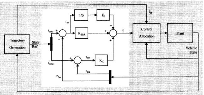
Perfect navigational information is presumed to be available for simulations presented in this text. All states of the dynamic system must be estimated or directly measured because the control law provided is full state. The algorithm is fundamentally a linear quadratic regulator (LQR) design that combines the functions of guidance and control. The rudiments of the design are taken from [13]. A block diagram of the LQR can be seen in Figure 3-4. The design differs from a pure LQR in two senses. First, the regulator portion of the title has been dropped in favor of servo. When applied to a flight control problem, the algorithm aims to track commands rather than to regulate about a set point. In this case the commands are the state variables acquired from the trajectory generation block. Because these trajectory commands correspond to a trimmed vehicle state, the LQ-Servo makes small corrections about trim. Consequently, aerosurface commands issued by the control allocation algorithm are applied with respect to feed-forward trimmed aerosurface positions, also provided by the

trajectory generator. The second deviation from pure LQR theory is the addition of

integrators. Specific vehicle states are integrated in order to guarantee zero steady-state error on those particular states. Table 3-5 supplements Figure 3-4 by identifying variables in the block diagram.

(35)

Figure 3-4. LQ-Servo with Integrators

Table 3-5. LQ-Servo Variable Definitions

Symbol Description

rcmd Tracking Commands: y, h, V rmeas Tracking Feedback

ren Tracking Error: integrated for zero steady-state error

Scmd State References: y, X, g, a, P, P,

Q,

R smeas State Feedback

seff State Error K,ERRi,X Control Gains

u Control Commands: roll, pitch, and yaw torque + speed brake command

Note the choice of control variables; three are generalized rotational commands while the fourth is dedicated to an aerodynamic actuator. The control allocation algorithm assigns control responsibility amongst the entry actuators (Table 3-2) but the speed brake is excluded from this selection. The LQ-Servo produces a speed brake command and simply passes it through the control allocation block and into the plant model. This decision was made because the speed brake modulates to induce drag, which in turn affects velocity. The ability

(36)

to exact translational control separates the speed brake from the other actuators, all of which are primarily used to induce moments, not forces. Both translational and rotational control requests can be satisfied through the use of a control allocation algorithm. However, because direct translational control is usually accomplished by rotating the vehicle with respect to the relative wind, the LQ-Servo is not configured to deliver generalized force commands. Potential application extensions involving direct translational control will be mentioned in the final chapter.

Control gains also deserve mention because they significantly affect the performance of the LQ-Servo. Similar to the trajectory references, control gains are calculated off-line and stored in table format. For simplicity in computation and implementation, time-invariant, steady-state LQR theory is used to calculate gains rather than applying optimal control principles. Because the vehicle model is a varying dynamic system, invoking a time-invariant routine. involves multiple operating points at which LQR gains are calculated. The trajectory consists of a finite number of reference points; at each reference point a linear system is created to emulate the vehicle dynamics (Equation (3.1)). When sequentially applied as the vehicle travels along the trajectory, these linear models with time-invariant coefficients replicate the nonlinear, time-varying dynamic behavior of the entry vehicle. LQR theory provides control gains by solving an optimization problem [14]. Consider the linearized system dynamics given in Equation (3.1), where A and B are constant coefficient matrices and [ A B ] is assumed to be stabilizable.

x = Ax- + Bfi (3.1)

A quadratic cost functional is defined based on the vectors of state variables, -, and control

variables, U-.

J =

J['Qi

+ iJ

R-]dt

(3.2)

0

Control gains are found by minimizing the cost, J, which involves solving the algebraic Riccati equation. Again, for a more detailed explanation of LQR theory and gain calculation please see [13,14].

(37)

The focus here will rest on the

Q

and R matrices; these are quantities that the designer uses

to adjust the characteristics of the controller. Matrix

Q

is the state weighting matrix and R is the control weighting matrix. These matrices are used to specify the relative importance of

minimizing both the state errors and control commands. Greater weighting on a state

variable tends to produce tighter tracking of the reference, while greater weighting on a control variable discourages its use as a control command. Because LQR is a multivariable technique, the controller simultaneously considers the effects of all control inputs on all state variables. This means that adjusting a single weighting parameter can have unpredictable effects on the controller characteristics. Techniques are available to guide the designer in selecting weightings, but trial-and-error is acceptable for this application because LQR design is not the focus of this research. The controller is implemented only to demonstrate the control allocation algorithm. Little attention is paid to robustness, disturbance rejection,

and sensitivity. Control performance is deemed acceptable provided that the vehicle

dynamics are stabilized, trajectory references are tracked, and the control bandwidths do not exceed the physical capabilities of the actuators.

To summarize this chapter, the equations of motion illustrate the vehicle response to its

environment, mass characteristics, and actuator states. These differential equations

accurately describe the X-34's dynamic behavior. Without compensation from a controller, the X-34's equations of motion reveal instability in the longitudinal plane due to the relative location of the center of mass and center of pressure. Trajectory references and full-state feedback are provided to a controller, which provides the required stability augmentation and tracking of the trajectory commands. The vehicle model demands actuator commands to provide forces and moments that will effect a stable vehicle attitude throughout entry. The speed brake position is calculated by the LQ-Servo and the control allocation algorithm provides the remaining aerosurface and RCS commands in response to LQ-Servo moment commands.

(38)

(39)

4 CONTROL ALLOCATION

Chapter 4 explains how the control allocation algorithm translates torque requests into actuator commands. The control allocation block executes a linear program to determine the optimal mix of bounded aerosurface deflections and RCS jet firings that yield the commanded vehicle response. Each actuator within the allocation framework possesses an activity vector, an objective function coefficient, and upper and lower bounds that determine its control authority, desirability, and hardware limits, respectively. The fundamentals of the linear program and supporting control allocation elements are presented in this chapter. Please consult Appendix A for a detailed account of the linear programming technique.

4.1 OVERVIEW

In most entry vehicle control frameworks, particular actuators are dedicated to controlling specific rotations during specific flight phases. Custom logic is often introduced to decouple actuators that possess control authority in multiple axes. Additionally, aerosurfaces are usually used in predetermined ways to compensate for aircraft instabilities. This method might lead to reduced efficiency and control margin, especially in the case of actuator

saturation or failure. The block diagram in Figure 4-1 displays an alternative to the

traditional approach.

(40)

Control allocation logic does not explicitly assign aerosurfaces to pre-specified channels. The control request is a generalized vehicle command about independently controlled axes, in this case torque commands (b), and all entry actuators are considered together in a common pool in an effort to satisfy these torque commands. Actuator control authorities are modeled by the activity vectors (A,), while actuator usage is encouraged or discouraged

through the objective function coefficients (c. ) and upper and lower bounds (UB, / LB,).

The value of each decision variable (x,) in the linear programming solution corresponds to action of an aerosurface or RCS jet family. Any aerosurface activity derived from the control allocation algorithm is applied with respect to the feed-forward trimmed aerosurface positions. RCS solutions must also be discretized into jet on/off commands by the pulsing logic block.

4.2 THE LINEAR PROGRAM

The linear program embedded within the control allocation design is summarized in the following statements and equations.

Minimize the objective function:

z = c ₁x 1 (4.1)

J=1

Subject to equality constraints...

n

AJ x./ = 5(4.2)

j=1

and inequality constraints:

LB, xj UB1 ; j e{ 1,2,...,n} (4.3)

where:

n = number of decision variables

x,= _{decision variable corresponding to control effort of aerosurface/RCS jet family}

(41)

UB, / LB, = upper/lower bounds associated with the th decision variable

Aj = activity vector representing the control authority of the th decision variable

b = generalized control command

Despite the purported use of linear programming, the objective function is nonlinear due to the absolute values. Aerosurface motion and RCS commands are unrestricted-in-sign and absolute values accomplish the goal of minimizing total control effort, both positive and negative. This presents an apparent contradiction between the objective function formulation and the prescribed linear programming technique. The algorithm resolves this dilemma by defining a weighted sum of nonnegative decision variables and a separate array containing their corresponding sign information. Algebraic operations are executed with nonnegative decision variables; this ensures that linear programming techniques are valid [15,16]. Using absolute values and separate sign information is not the typical approach when unrestricted-in-sign variables are involved. The conventional method expresses an unrestricted-unrestricted-in-sign decision variable x, as the difference of two nonnegative variables xj(a) and xJ(b) in each

constraint and in the objective function [15]. This action doubles the size of a problem when all variables are unrestricted-in-sign, as is the case in this application. The algorithm used in this application is a tidy way to account for unrestricted-in-sign variables without creating twice the number of decision variables.

The primary function of the linear program is to map control commands into actuator commands. It accomplishes this task by determining the values of the decision variables that satisfy the equality constraints. The objective function and inequality constraints specify

user-defined performance criteria and hardware feasibility limits, respectively. The

following bullet statements attempt to further clarify these three elements of the linear selection.

* Objective Function: Each objective coefficient is defined by the designer and is chosen to

encourage or discourage a particular actuator response. Because it is a minimization problem, assigning a coefficient of great magnitude to a decision variable penalizes the

(42)

use of the actuator corresponding to that decision variable. These coefficients, also referred to as costs or penalties, are dynamically updated between control cycles during

entry.

" Equality Constraints: These constraints define the feasible solution space of the decision

variables. Each A., corresponds to the ability of a particular actuator to offer

instantaneous rolling, pitching, and yawing moments (per unit value of decision variable). The number of equations comprising the equality constraints is equal to the number of independent control axes (i.e., 3 for rotational control only, 6 for rotation and translation). The calculation of activity vectors is customized for each actuator family and is discussed at a later point. The b vector comes from the vehicle controller and its dimension also reflects the number of control axes.

* Inequality Constraints: These constraints further define the solution space. They are

simply limits on the allowable value of each decision variable and might represent such

quantities as aerosurface displacement restrictions. Bounded decision variables are

necessary to ensure that the solutions of the linear program do not violate vehicle hardware constraints. Bounds, like objective function penalties, might also be used to promote particular actuator combinations.

The linear program solves the constrained optimization problem with a bounded

simplex-based algorithm. The simplex method is an algebraic procedure but it can easily be

illustrated through geometry. The following two-dimensional example problem affords

insight into the fundamentals of the algorithm.

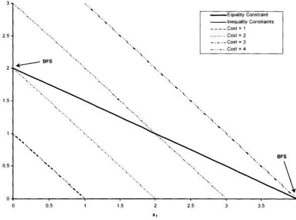
Example 1: minimize, z = x1 +x2

subject to,

[1

2]x] = 4

X ₂ _

(43)

In this example, the equality constraint corresponds to a line and no upper bounds are applied. Only the first quadrant is shown in Figure 4-2 because the non-negativity condition restricts the feasible solution space to this area. Solutions that satisfy both equality and inequality constraints lie along the line segment. Of particular note are the corner points, defined as intersections between constraint boundaries. An essential principle exploited by the simplex method is the fact that a basic feasible solution (BFS) exists at a corner point

[15,16]. 3 - Equality Constraint -Inequality Constraints ---- Cost = 1 2.5- ---.- Cost = 2 \ --- Cost = 3 -. _Cost = 4 - BF 2 1.5 -- 0.5-0 0 0.5 1 1.5 2 2.5 3 3.5 4 X1

Figure 4-2. Geometry of Example 1

To see why this statement is true, examine the family of parallel lines representing objective functions of increasing cost (e.g., I = x, + x2, 2 = x, + x2, etc...). The objective function with

zero cost intersects the origin. This is obviously the "cheapest" solution, but it does not satisfy all constraints because the objective function does not intersect the line segment representing the feasible solution space. The goal becomes straightforward: find the least expensive objective function that intersects the feasible solution space. From Figure 4-2 it is

(44)

apparent that, whether minimizing or maximizing an objective, a corner point always yields an optimal solution. Because this is true, the simplex method begins iterations at a corner point and searches for the optimal solution by moving along constraint boundaries to adjacent corner points. The simplex method finds efficiency in limiting the search to only these corner point solutions. Iterations continue until a move to any other adjacent corner point cannot improve the current solution. When this occurs, the algorithm returns the current corner point and associated cost because this must be an optimal solution. In the minimization example problem the optimal solution is the point (0,2) with a cost of 2. Likewise, the other corner point solution, the point (4,0) with a cost of 4, is the optimum to the maximization problem.

The same principle applies when the problem is extended beyond two dimensions. During simulation there are n decision variables, n inequality constraints, and m equality constraints. Now the feasible region is no longer a line segment but a set of hyperplanes in

n -dimensional space. Still, the solution yielding the minimum cost is found by testing

feasible combinations of the n activity vectors. With each iteration activity vectors are swapped in and out of the solution. This corresponds to a switch between corner points within the feasible solution space. If the problem is properly posed, an activity vector exchange is only executed if it will improve, or at least maintain, the evaluation of the objective function.

4.2.1 Blending Techniques

One purpose of introducing control allocation logic is to blend the effects of aerosurfaces and RCS jets during the control effector transition as the vehicle enters the atmosphere. This can be accomplished in one of two ways. The first method is to use the bounds to redefine the feasible solution space. The linear objective function applied to both the example problem and this research effort is effective in minimizing control effort because nonzero decision variables are discouraged. However, if no upper bounds are actively enforced, the corner point solutions from this objective formulation contain only as many nonzero decision variables as equality constraints. The example problem has one equality constraint equation. Whether minimizing or maximizing the objective function, only one decision variable

(45)

contributes a nonzero value to the optimal solution. All other decision variables must be zero, otherwise the result is a feasible solution but not an optimal solution. Now consider the

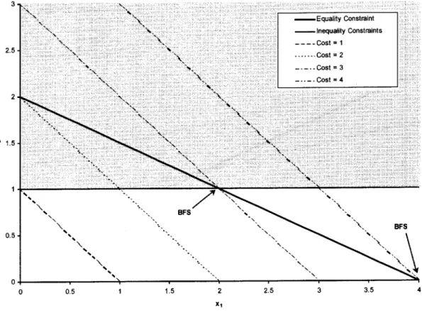
same example problem with an upper bound of one applied to x2. The geometry of this

problem is shown in Figure 4-3. The solution space shrinks because answers containing x, greater than one are infeasible. Minimizing the objective function results in an optimal solution at (2,1) with a cost of 3. Note the nonzero contributions of both decision variables despite the fact that there is still only a single equality constraint equation. This concept also finds application in the simulation environment. During rotational control, when the number of equality constraints equals three, the optimal solution will utilize only three actuators if the upper bounds are inactive. Active upper bounds force the control allocation solution to include the effects of a greater number of actuators rather than force the action of the minimum number of control effectors.

3 4 - Equality Constraint Inequality Constraints ---- Cost = 1 2.5 -.-Cost = 2 - --- Cost = 3 -.. Cost = 4 2-1.5' BFS BFS 0.5 -0 o0.5 1 1 .5 2 2.5 3 3.5 4 X1

Figure 4-3. Geometry of Example 1 with Upper Bound onx2

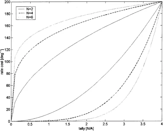
The other means by which the linear program can induce blending is through the objective coefficients. This method relies on the dynamic calculation of objective penalties between

(46)

control cycles. Consider the original example problem's constraints and objective function to be a product of simulation at some initial time. The ensuing time step, with new control commands and linear selection, might yield identical constraints but a different objective.

Figure 4-4 displays such a case. The decision variable x2, in response to some

environmental factor, is now four times more expensive in the objective function. The optimal solution to the minimization problem is no longer (0,2); it has shifted to the point

(4,0). Increasing the objective penalty on x2 removed it from the solution and it was

replaced entirely by x₁. With regard to the entry application, this sort of substitution of one decision variable for another in successive control cycles could represent the dynamic effector transition from RCS yaw jets to rudder.

- Equality Constraint - Inequality Constraints ---- Cost = 2 -. ... Cost = 4 --- Cost = 6 --- Cost = 8 BFS BFS 0 0.5 1 1.5 2 2.5 X1 3.5

Figure 4-4. Geometry of Example 1 with Objective Function z = x I+4 -x21

The latter blending approach is adopted in this research effort. During simulation, LQ-Servo commands are issued every 20 milliseconds. The linear program must also allocate control

3 2.5 2 2 1.5 1 0.5 0