HAL Id: hal-02270791
https://hal-amu.archives-ouvertes.fr/hal-02270791
Submitted on 26 Aug 2019
HAL is a multi-disciplinary open access
archive for the deposit and dissemination of
sci-entific research documents, whether they are
pub-lished or not. The documents may come from
teaching and research institutions in France or
abroad, or from public or private research centers.
L’archive ouverte pluridisciplinaire HAL, est
destinée au dépôt et à la diffusion de documents
scientifiques de niveau recherche, publiés ou non,
émanant des établissements d’enseignement et de
recherche français ou étrangers, des laboratoires
publics ou privés.
Banking stability, natural disasters, and state fragility:
Panel VAR evidence from developing countries
Pedro Albuquerque, Wassim Rajhi
To cite this version:
Pedro Albuquerque, Wassim Rajhi. Banking stability, natural disasters, and state fragility: Panel
VAR evidence from developing countries. Research in International Business and Finance, Elsevier,
2019, 50, pp.430-443. �10.1016/j.ribaf.2019.06.001�. �hal-02270791�
Banking stability, natural disasters, and state fragility: Panel VAR
evidence from developing countries
Pedro H. Albuquerque
a,⁎, Wassim Rajhi
ba KEDGE Business School, Marseille, France & Aix-Marseille Univ., CNRS, EHESS, Centrale Marseille, IRD, AMSE, Marseille, France b Independent Researcher JEL classifications: G21 O57 Keywords: Banking stability GDP per capita Natural disasters State fragility A B S T R A C T
Panel VAR methodology is used in this study to empirically evaluate the effects of natural dis-asters and state fragility on economic and financial dimensions in developing countries such as GDP per capita, banking and financial system deposits, banks’ Z-scores, and non-performing loans. Results based on three panels of up to 66 countries and 17 years of annual data indicate that natural disasters and state fragility may cause significant economic and financial disruption in low-income and middle-income countries. Shocks from natural disasters seem to be temporary and detrimental only to non-performing loans, while shocks from state fragility appear to be permanent and to create detrimental economic and financial feedback loops.
1. Introduction
The economic literature on natural disasters is typically concerned with its impacts on macroeconomic variables such as GDP per capita and economic growth. For example,Hallegatte and Ghil (2008)find that the average production loss due to a set of disasters distributed in time at random is highly sensitive to the dynamical characteristics of the impacted economy.Noy (2009)shows that, when subject to disasters of similar relative magnitudes, developing countries face much larger output declines than do developed countries.Klomp and Valckx (2014)find that climatic disasters have the most significant adverse impacts on economic growth in developing countries.Anuchitworawong and Thampanishvong (2015)show that severe natural disasters tend to lower FDI flows into Thailand, whileDoyle and Noy (2015)find that earthquakes reduce CPI inflation moderately and have an adverse effect on real GDP growth.
Concerning the mediation of institutional and political dimensions, countries with higher literacy rates, better institutions, higher per capita income, higher degree of openness to trade, and higher levels of government spending are better able to withstand a disaster shock and prevent further spillovers into the economy.Hoon Oh and Reuveny (2010)show that disaster incidence and political risk in an importer or exporter country reduce trade.Dell et al. (2012)find that higher temperatures reduce political stability and economic output in developing countries.Cavallo et al. (2013), on the other hand, find that, once the negative effects of subsequent radical political revolutions are controlled for, natural disasters do not display any significant effect on economic growth. The economic literature on political instability is also typically concerned with its relations with major macroeconomic dimen-sions. It is generally agreed that political instability adversely affects growth by lowering rates of productivity growth and physical and human capital accumulation, reducing long-run economic growth, as shown inJong-A-Pin (2009)andAisen and Veiga (2013).
Brada et al. (2006)find that the FDI flows to transition economies unaffected by conflict and political instability exceed those that
⁎
Corresponding author at: KEDGE Business School, Domaine de Luminy BP 921, 13288 Marseille, France.
E-mail address:[email protected](P.H. Albuquerque).
would be expected for comparable West European countries.Uddin Ahmed and Habibullah Pulok (2013)show that political in-stability has a negative effect on economic performance in the long run while having a positive short-run effect in Bangladesh.Aisen and Veiga (2008)find that political instability generates higher inflation rates and seigniorage.
The financial literature in its turn has given considerable attention recently to delineating institutions that foster or impede financial development. Financial market services should normally enhance economic growth due to improved market liquidity (Rajan and Zingales, 1998;Levine and Zervos, 1998;Levine, 2005). Poor corporate governance and management are often compounded by weak legal and judicial infrastructures, particularly in developing countries. Inadequate corporate, bankruptcy, contract and property law as well as ineffectual judicial enforcement contribute to a breakdown in credit discipline, leading to a higher incidence of non-performing loans.Jokipii and Monnin (2013)show that an unstable banking sector increases uncertainty about future output growth. Countries lacking a sound legal system tend to have more financial system problems due to inefficient law enforcement and to government ineffectiveness (La Porta et al., 1998;Levine and Zervos, 1998;Fernandez and González, 2005).
Čihák and Tieman (2011)have demonstrated that in high-income countries the quality of financial sector regulation is higher than that in low-income countries, therefore the impacts of natural disasters and political instability on financial and banking stability are expected to be more significant in developing countries. These impacts remain however relatively unexplored since most of the literature, as mentioned above, is concerned with its effects on major macroeconomic variables such as output and long-run economic growth.
Four factors are known to cause financial instability in developing countries: (i) unexpected increases in interest rates, (ii) a deterioration in bank balance sheets, (iii) negative shocks to nonbank balance sheets, such as a stock market decline, and (iv) increases in uncertainty. These four factors may be triggered or amplified by natural disasters and political instability.Demirgüç-Kunt and Detragiache (1998)find that crises tend to erupt when growth is low and inflation is high. They also find banking sector problems to be related with high real interest rates, vulnerability to balance of payments crises, existence of an explicit deposit insurance scheme, and weak law enforcement.Kaminsky and Reinhart (1999)find that banking crises coincide with balance of payments crises in developing countries, what increases the fragility of the banking system even further.Beck et al. (2006)suggest that crises are less likely in economies with more concentrated banking systems, even after controlling for the differences between conventional bank regulatory policies, national institutions affecting competition, macroeconomic conditions, and shocks to the economy. The authors find evidence that more concentrated banking systems offer more possibilities for banks to diversify risk.
Natural disasters and political instability can also be understood as banking operational risks. According to the Basel Committee, operational risk is defined as “the risk of loss resulting from inadequate or failed internal processes, people and systems or from external events. Operational risk factors incorporate mismanagement, inadequate staffing, malfunctions in information processing systems, weak control systems, fraud and catastrophic events” (Basel Committee on Banking Supervision, 2010). To ensure the continuity of operations in the event of a natural disaster or state failure, and to minimize any disruption to customers, banks and markets, banks need to address these events as operational risks that can adversely affect the smooth functioning of the financial system, i.e., financial markets, payments, settlement and clearing systems.
Despite this possible direct relationship between natural disasters and banking stability, many studies provide only indirect evidence of it, as they study isolated risk aspects (capital ratios, loan portfolio quality) or activities (credit supply, deposits).Noy (2009)argues that countries with more foreign exchange reserves and higher levels of domestic credit but with less open capital accounts appear to be more robust and better able to endure natural disasters, with less adverse spillover into domestic production.
David (2011) points out that bank lending activities reduce rapidly after a climatic disaster in developing countries. Berg and Schrader (2012)analyze the effects of unpredictable aggregate shocks on loan demand and access to credit by combining client-level information from an Ecuadorian microfinance institution. The results show that while credit demand increases due to volcanic activity, access to credit is restricted. They also find that bank-borrower relationships can lower these lending restrictions and that clients who are known to the institution are about equally likely to receive loans after volcanic eruptions occurred.
Klomp and de Haan (2015)show that capital requirements and supervision reduce the likelihood of bank defaults in developing countries.Collier and Skees (2013)find that developing economies are more vulnerable to certain systemic risks such as natural disasters, and that jurisdictions vulnerable to disasters hold slightly greater capital reserves than those in less vulnerable regions. Using a comprehensive dataset of commercial banks,Klomp (2014)showed that natural disasters increase the likelihood of banks’ defaults due to the widespread damage they create, which depletes banks’ reserves and increases leverage.
This article contributes to the literature by using panel VAR methodology to empirically examine the links among natural dis-asters, state fragility (a source of political instability), financial and banking risk and economic output. The models are based on three panel datasets of sizes varying from 34 to 66 developing countries and from 12 to 17 years of annual data (1995–2011).1The paper is structured as follows: Section2outlines the data and empirical methodology, Section3describes the results, and Section4contains the concluding remarks. The study’s contribution consists in empirically demonstrating that the impact of natural disasters and state fragility on the economic, financial and banking stability of developing countries can be economically significant (as defined in
Goldberger, 1991, pg. 240) and statistically significant.
1Low-income countries are defined by theWorld Bank (2013)as those with a Gross National Income (GNI) per capita, of $1,045 or less;
middle-income countries are those with a GNI per capita of more than $1,045 but less than $12,736; lower-middle-middle-income and upper-middle-middle-income countries are separated at a GNI per capita of $4,125. High-income countries are those with a GNI per capita of more than $12,736. Developing countries are defined here as all but high-income countries.
Variable Det. Maddala-Wu Choi's modified P Choi's inverse normal Im-Pesaran-Shin GDP per capita c, t 0.004*** 0.002*** 0.998 0.948 GDP growth c, t 0.000*** 0.000*** 0.000*** 0.000*** Banks’ Z-scores c, t 0.000*** 0.000*** NA 0.000*** Banking deposits c, t 0.000*** 0.000*** 0.000*** 0.000*** Financial system deposits c, t 0.000*** 0.000*** 0.000*** 0.000*** Non-performing loans c 0.000*** 0.000*** NA 0.000*** Lifeyears lost index c, t 0.000*** 0.000*** 0.000*** 0.000***
State fragility index any NA NA NA NA
Null hypothesis of nonstationarity, SIC used as lag selection criterion, maximum lag = 4, Det.=deterministic components, c = intercept, t = time trend, any = any deterministic component combination including none, NA = not available, statistical significance: * = 10%, ** = 5%, *** = 1%. Table 2
Panel Granger causality tests, x does not Granger cause y, p-values.
Y x GDP per
capita GDP growth Banks’ Z-scores Bankingdeposits Financial systemdeposits Non-performingloans Lifeyears lostindex State fragilityindex GDP per capita 0.000*** 0.000*** 0.000*** 0.284 0.089* 0.000***
Panel 2 Panel 1 Panel 1 Panel 3 Panel 1 Panel 1 2 lags 3 lags 3 lags 2 lags 3 lags 1 lag GDP growth 0.344 0.260 0.049** 0.694 0.974 0.570
Panel 2 Panel 1 Panel 1 Panel 3 Panel 1 Panel 1 2 lags 3 lags 3 lags 2 lags 3 lags 1 lag
Banks’ Z-scores 0.259 0.215 0.699 0.887
Panel 2 Panel 2 Panel 2 Panel 2
2 lags 2 lags 2 lags 2 lags
Banking deposits 0.000*** 0.000*** 0.001*** 0.000***
Panel 1 Panel 1 Panel 1 Panel 1
3 lags 3 lags 3 lags 1 lag
Financial system
deposits 0.000*** 0.000*** 0.015** 0.000***
Panel 1 Panel 1 Panel 1 Panel 1
3 lags 3 lags 3 lags 1 lag
Non-performing loans 0.233 0.250 0.173 NA
Panel 3 Panel 3 Panel 3 Panel 3
2 lags 2 lags 2 lags all
Lifeyears lost index 0.000*** 0.000*** 0.978 0.838 0.887 0.493 Panel 1 Panel 1 Panel 2 Panel 1 Panel 1 Panel 3 3 lags 3 lags 2 lags 3 lags 3 lags 2 lags State fragility index 0.000*** 0.000*** 0.004*** 0.000*** 0.000*** NA
Panel 1 Panel 1 Panel 2 Panel 1 Panel 1 Panel 3 2 lags 2 lags 2 lags 2 lags 2 lags all
Null hypothesis is x does not Granger cause y for all countries, maximum lag = 3, NA = not available, all = any lag selection, statistical significance: * = 10%, ** = 5%, *** = 1%.
Table 3
Panel VAR models.
Dataset Lags Variable A (most contemporaneously exogenous
innovations) Variable B Variable C (least contemporaneously exogenousinnovations) Model 1 Panel 1 2 State fragility index GDP per capita Banking deposits
Model 2 Panel 1 2 State fragility index GDP per capita Financial system deposits Model 3 Panel 2 2 State fragility index GDP per capita Banks’ Z-scores Model 4 Panel 3 2 State fragility index GDP growth
(exogenous) Non-performing loans Model 5 Panel 1 2 Lifeyears lost index GDP per capita Banking deposits Model 6 Panel 1 2 Lifeyears lost index Financial system deposits Model 7 Panel 2 2 Lifeyears lost index Banks’ Z-scores Model 8 Panel 3 2 Lifeyears lost index Non-performing loans
Estimated using two-step GMM, forward orthogonal deviations, and the collapse option. Table 1
2. Data and empirical methodology
2.1. Data
The following variables were used to create a set of country and annual data: (i) GDP per capita (lngdppc) or (ii) GDP growth (dlngdppc), (iii) banks’ Z-score (lnzscore), (iv) banking deposits (lnbdgdp), (v) financial system deposits (lnfdgdp), (vi) non-per-forming loans (lnnltl), (vii) lifeyears lost index (lgtlfyl), and (viii) state fragility index (lnsfi). These variables and their sources are described in detail in Appendix1. To optimize information available to the models, 3 panel datasets were built containing the largest possible numbers of developing countries and annual observations in the data for different combinations of variables. The lists of variables, time ranges and countries for each of the 3 panel datasets are given in Appendix2.
Variables such as non-performing loans, which measure loan risks, may be well known and commonplace in the literature but they are also known to be lagging indicators of banking soundness (Schaeck and Čihák, 2014). Therefore, a measure of distance-to-default, the banks’ Z-scores, is also employed in this study. Banks’ Z-scores measure the market value of banks’ assets in relation to the book value of their liabilities, meaning that they also measure the distance from insolvency by combining accounting information on profitability, leverage and volatility. Banks’ Z-scores are inversely related to the probability of banks’ insolvency, i.e., the probability that the value of its assets will become lower than the value of the debt.2Higher banks’ Z-scores correspond to lower risk of insolvency. Insolvency is defined byBoyd and Runkle (1993)as a realization of profits ˜ in which losses exceed equity E. The probability of failure can be defined as:
< = < = = = p E p r k r r r A k E A ( ˜ ) (˜ ) (˜)d , ˜ ˜, k (1) where A is bank assets and, if r is normally distributed, (1) may be rewritten as:
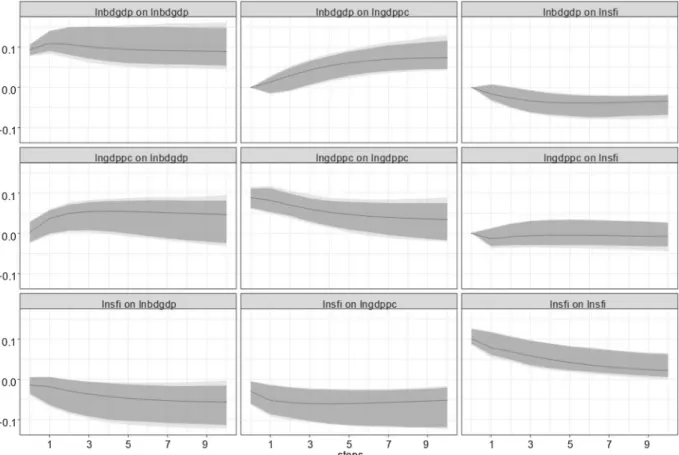
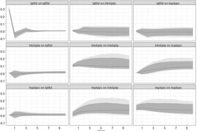
Fig. 1. Orthogonalized impulse response functions, model 1OIRFs and 90% (dark), 95% (light) confidence bands. 10 years ahead, lnsfi = state fragility index, lngdppc = GDP per capita, lnbdgdp = banking deposits.
2Banks’ Z-scores do not rely on the subjective judgment of rating agencies’ analysts. The advantage of using the Z-score as a measure of bank
< = p r(˜ k) N(0,1)dz z (2) = + z (k )/ (3)
where is the true mean of the r distribution, is the true standard deviation, and z is the number of standard deviations below the mean by which r would have to fall to remove equity. Because of the Bienayme-Tchebycheff inequality, even when r is not normally distributed, z indicates the lower bound on the probability of failure given and . Eqs.(1)–(3)suggest that an increase in the intensity of natural disasters and of state fragility should reduce the distance-to-default within the banking sector.
The natural disaster variable used in this article is based on the Disability Adjusted Lifeyears (DALYs) measure developed byNoy (2015). This lifeyears lost index is chosen because it smoothens out higher values of lifeyears lost. It converts all damage indicators into an aggregate measure of human lifeyears lost.3Lifeyears lost due to mortality are calculated as the difference between the age at death and life expectancy. The cost in lifeyears associated with people who were injured (or otherwise affected by the disaster) is assumed to be defined as a function of the degree of disability associated with being affected, multiplied by the duration of this disability, times the number of people affected. Low-income countries experience by far the highest per capita burden and high-income countries account for a very small share of the overall burden due to natural disasters (Noy, 2015).
The chosen political instability variable is the state fragility index developed by the Integrated Network for Societal Conflict Research (INSCR,Cole and Marshall, 2014). The state fragility index rates each country according to its level of fragility in both effectiveness and legitimacy across four development dimensions: (i) security, (ii) political, (iii) economic, and (iv) social. This measure of fragility is designed to provide comparable and objective levels of development of societal systems around the world. Decreases in state fragility are equivalent to increases in societal system resiliency. State fragility is for example closely related to warfare in developing countries.
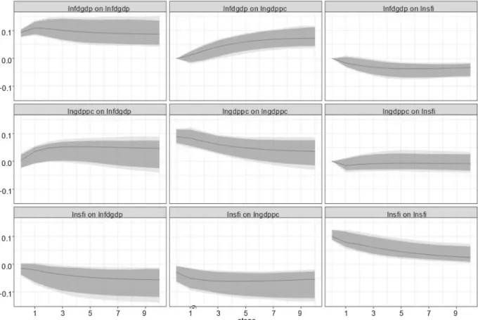
Fig. 2. Orthogonalized impulse response functions, model 2 OIRFs and 90% (dark), 95% (light) confidence bands. 10 years ahead, lnsfi = state fragility index, lngdppc = GDP per capita, lnfdgdp = financial system deposits.
2.2. Empirical methodology
The main objective of this article is to investigate how natural disasters and state fragility may affect economic, financial and banking systems of developing countries. In order to do so, 8 panel VAR models are estimated based on the 3 panels of data described in the previous subsection.
The empirical modelling strategy uses the following steps: (i) panel unit root tests are used to verify if variables are stationary or not, (ii) if two or more variables in a model are assumed to be nonstationary, panel cointegration tests are performed to assess the need to employ cointegration models, (iii) panel Granger causality tests are used to identify possible predictive relations among variables in the dataset, (iv) parsimonious panel VAR models are selected using stability and information criteria and then estimated, and (v) interpretations are outlined based on orthogonal impulse response functions (OIRFs) with bootstrap confidence bands and forecast error variance decompositions (FEVDs).
In what follows, R version 3.5.3 was used as econometric package (R Core Team, 2019). The following specialized R libraries were also employed: plm version 1.7-0 was used for panel unit root tests (purtest) and panel Granger causality tests (pgrangertest), see
Croissant and Millo (2008)andKleiber and Lupi (2011), and panelvar version 0.5.2 was used for panel VAR model selection, estimation and interpretation, seeSigmund and Ferstl (2019).
3. Results
3.1. Panel unit root tests
Table 1shows panel unit root test results for the selected variables. Four types of tests were employed: (i) Maddala-Wu is the inverse chi-squared test presented inMaddala and Wu (1999), also called P test byChoi (2001); (ii) Choi’s modified P and (iii) Choi’s inverse normal are both tests described inChoi (2001); and (iv) Im-Pesaran-Shin is the test proposed inIm et al. (2003). Schwarz information criterion (SIC) was used as lag selection criterion in all tests, and deterministic components preferentially included intercept and time trend, unless leading to unavailable results, in which case they were reduced to intercept only, and finally to no deterministic component if necessary.
Panel unit root test results indicate that the null hypothesis of nonstationarity (unit roots present for all countries) is strongly
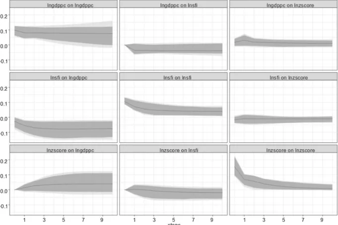
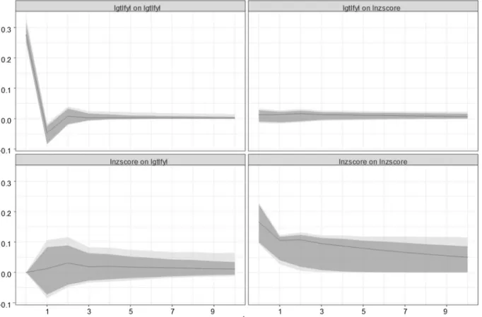
Fig. 3. Orthogonalized impulse response functions, model 3 OIRFs and 90% (dark), 95% (light) confidence bands. 10 years ahead, lnsfi = state fragility index, lngdppc = GDP per capita, lnzscore = banks’ Z-score.
rejected. The only exception is GDP per capita, for which the null hypothesis of nonstationarity is not rejected by two among the four tests. Results for the state fragility index were not available, probably due to the bounded, discrete and synthetic nature of this variable.
Given that only one variable is possibly nonstationary, panel cointegration testing is not necessary. Panel VAR models do not suffer from inconsistent estimates (spurious regression) due to nonstationary variables (Phillips and Moon, 2000), so the choice in this article is to preserve long-run information by not applying the first-difference transformation to GDP per capita unless necessary.
3.2. Panel granger causality tests
Panel Granger causality is evaluated using the test proposed inDumitrescu and Hurlin (2012). Lag selection criteria was the following: when possible 3 lags were used (this was the longest possible lag structure for the largest dataset). If results with 3 lags were unavailable, lag length was reduced until results became available.
Table 2shows p-values for the panel Granger causality tests for each pair of variables associated to one of the 8 panel VAR models to be estimated. Results can be summarized as follows. Firstly, GDP growth is less able to Granger cause other variables than GDP per capita: tests only reject noncausality once for the latter, supporting the strategy of using variable levels instead of first-difference transformations whenever possible.
Secondly, the null hypothesis that non-performing loans does not Granger cause or is not granger caused by other variables is never rejected. This result may be a consequence of the smaller size of panel 3, but in any case, it suggests that models including this variable may perform less well than other models. And thirdly, banks’ Z-scores tend to be Granger caused by other variables but to not Granger cause them (the null hypothesis that this variable does not Granger cause any other variable is never rejected).
These three results suggest that the following contemporaneous exogeneity order for innovations in the panel VAR models may be adequate: lifeyears lost index and state fragility index are set as the most contemporaneously exogenous, followed by GDP per capita, and finally by financial variables as the least contemporaneously exogenous.
3.3. Panel VAR model selection and estimation
Panel VAR models were selected based on stability and information criteria (SIC). Unstable models containing eigenvalues with
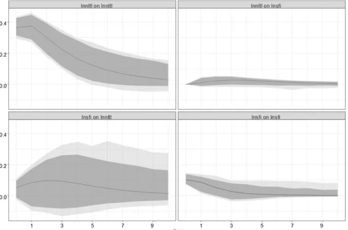
Fig. 4. Orthogonalized impulse response functions, model 4 OIRFs and 90% (dark), 95% (light) confidence bands. 10 years ahead, lnsfi = state fragility index, lnnltl = non-performing loans.
modulus greater than one were discarded. Among stable models, lags were selected using information criteria (SIC), starting with a minimum of 2 lags. In some cases stability was achieved by setting GDP per capita or GDP growth as an exogenous variable or, when not statistically significant, through the exclusion of GDP per capita or GDP growth from the model. Maybe because of small panel sizes, models with four variables were unstable or had unstable OIRFs, so the analysis in what follows remains restricted to three-variable panel VAR models.
Table 3describes the 8 chosen panel VAR models estimated using two-step GMM and forward orthogonal deviations. All models have at least three coefficients that are statistically significant at the 5% level. The null hypothesis of valid overidentification re-strictions was never rejected according to the results of the Sargan-Hansen J-test.
3.4. Orthogonal impulse response functions (OIRFs)
Estimated OIRFs with 90% and 95% confidence bands were obtained through 1000 bootstrap draws and are shown inFigs. 1–8. Models 1 and 2, seen inFigs. 1 and 2, display the interactions among political instability innovations (represented by the state fragility index), economic output innovations (represented by GDP per capita), and banking and financial stability (represented by banking deposits and financial system deposits). State fragility innovations lead to economically and statistically significant (5% significance level) permanent decreases in both GDP per capita and banking and financial system deposits. GDP per capita in-novations lead to economically and statistically significant permanent increases in banking and financial system deposits. Banking deposits or financial system deposits innovations lead to economically and statistically significant permanent increases in GDP per capita and permanent decreases in state fragility. In summary, state fragility shocks tend to create economically and financially detrimental feedback loops.
Model 3 uses banks’ Z-scores instead of deposits to represent financial stability.Fig. 3shows responses that are like those ofFigs. 1 and 2, but the effects on banks’ Z-scores are generally less economically significant (as measured by the magnitudes of the IRFs) and the only statistically significant relation at the 5% significance level concerns the effects of state fragility on GDP per capita. Otherwise, relations tend to not be statistically significant or are only close to be statistically significant at the 10% significance level. These results are possibly driven at least in part by a smaller panel size due to limited data availability for banks’ Z-scores.
Model 4 indicates that state fragility index innovations have an economically significant effect on non-performing loans, but never statistically significant (10% confidence level), as seen inFig. 4. Lack of statistical significance, as mentioned before, may be at least partially related to the small size of panel dataset 3.
Fig. 5. Orthogonalized impulse response functions, model 5 OIRFs and 90% (dark), 95% (light) confidence bands. 10 years ahead, lgtlfyl = lifeyears lost index, lngdppc = GDP per capita, lnbdgdp = banking deposits.
Models 5, 6, 7 and 8 use the lifeyears lost index to represent natural disasters. OIRFs for models 5, 6 and 7, shown inFigs. 5–7, indicate that lifeyears lost index innovations have little effect on GDP per capita and on broader financial variables, such as banking and financial system deposits and banks’ Z-scores, with effects that are neither economically nor statistically significant at the 10% significance level.
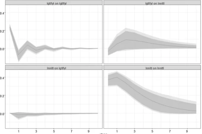
Model 8′s IRFs shown inFig. 8indicate that lifeyears lost index innovations lead to economically significant and, for some step ahead values, statistically significant effects on non-performing loans at the 10% significance level. Its responses are temporary though, waning after a few years, in contrast to the permanent nature of state fragility responses.
Our main findings suggest that political instability tends to permanently reduce economic output and banking and financial system deposits, while natural disasters seem to temporarily increase the amount of non-performing loans, therefore both types of shocks may increase the likelihood of bank defaults in developing countries, depleting banks’ reserves and increasing their leverage.4 Additionally, the impulse response functions for GDP per capita tend to be in agreement with the meta-analysis inLazzaroni and Van Bergeijk (2014)as they suggest that natural disasters have no or negligible effect on economic performance. The results for the state fragility index are also consistent with previous studies that show that political instability can be economically costly.
3.5. Forecast error variance decompositions (FEVDs)
While OIRFs examine the responses of a variable to other variables’ innovations, FEVDs indicate the contribution of each vari-able’s innovation to the determination of other variables’ forecast error variances, being therefore a good indicator of economic significance. The FEVDs proportions after 10 years are given inTables 4 and 5. Results can be summarized as follows.
Firstly, state fragility index innovations normally contribute much more significantly to banking and financial variables and to GDP per capita in the long run than lifeyears lost index innovations do, in agreement once again with the meta-analysis inLazzaroni and Van Bergeijk (2014). This also confirms that responses to state fragility innovations, as mentioned in the previous subsection, are
Fig. 6. Orthogonalized impulse response functions, model 6 OIRFs and 90% (dark), 95% (light) confidence bands. 10 years ahead, lgtlfyl = lifeyears lost index, lnfdgdp = financial system deposits.
4The securitization structures introduce additional risk through linkages between financial institutions. When catastrophe strikes, retrocession to
other financial institutions uses contractual arrangements between reinsurers and commits banks and other financial institutions to pay out when the retroceded risk materializes. Among insurance-linked securities, catastrophe bonds are the main instrument for transferring reinsured disaster risks to financial markets (Von Dahlen and Von Peter, 2012).
economically significant. Secondly, GDP per capita innovations have significant participation in the long-run determination of banking and financial variables. Thirdly, long-run GDP per capita receives significant contributions from all financial variables. And fourthly, FEVD analysis confirms that the contribution of lifeyears lost index to long-run non-performing loans is relatively small but economically significant.
4. Conclusions
This article examined the relationships between natural disasters, state fragility, banking and financial risk, and output. Using up to 66 developing countries and 17 years (1995–2011) of data, 8 panel VAR models were used to examine the links among lifeyears lost, state fragility, GDP per capita, banking and financial system deposits, banks’ Z-scores, and non-performing loans.
Impulse response function analysis yielded significant empirical findings. Natural disasters and state fragility are both econom-ically and financially disruptive. State fragility shocks tend to permanently reduce GDP per capita and banking and financial system deposits and to create detrimental feedback loops, while natural disaster shocks appear to temporarily increase the amount of non-performing loans. In any case, both shocks may increase the likelihood of bank defaults in developing countries. These results are consistent with earlier studies showing that natural disaster shocks do not have broad economic and financial consequences, while political instability can be economically costly in the short and long run. Variance decomposition analysis confirmed that state fragility innovations can have economically significant long-run effects on economic and financial dimensions.
Lifeyears lost and state fragility were empirically shown to be among the many factors that can influence banking and financial variables. This article is consequently of interest to a strand of macroeconomic and financial literature that deals with the economic and financial impacts of natural disasters and political instability. This topic is relevant to policymakers as well: from a prudential point of view, policy could be designed to increase bank reserves and reduce leverage during lasting periods of political instability or when natural disaster risks are substantial.
Fig. 7. Orthogonalized impulse response functions, model 7 OIRFs and 90% (dark), 95% (light) confidence bands. 10 years ahead, lgtlfyl = lifeyears lost index, lnzcore = banks’ Z-score.
Fig. 8. Orthogonalized impulse response functions, model 8 OIRFs and 90% (dark), 95% (light) confidence bands. 10 years ahead, lgtlfyl = lifeyears lost index, lnnltl = non-performing loans.
Table 4
Forecast error variance decompositions (FEVDs) of banking & financial variables 10 years ahead.
Variable Innovation A Innovation B Innovation C Model 1 State fragility index GDP per capita Banking deposits
Banking deposits 13.3% 17.1% 69.6%
Model 2 State fragility index GDP per capita Financial system deposits Financial system deposits 13.9% 16.3% 69.8%
Model 3 State fragility index GDP per capita Banks’ Z-scores
Banks’ Z-scores 3.2% 7.1% 89.7%
Model 4 State fragility index Non-performing loans
Non-performing loans 8.4% 91.6%
Model 5 Lifeyears lost index GDP per capita Banking deposits
Banking deposits 1.9% 26.8% 71.3%
Model 6 Lifeyears lost index Financial system deposits
Financial system deposits 0.3% 99.7%
Model 7 Lifeyears lost index Banks’ Z-scores
Banks’ Z-scores 1.5% 98.5%
Model 8 Lifeyears lost index Non-performing loans
Acknowledgements
The authors are thankful for comments and suggestions from anonymous referees and from members of the SEEFAR (Shift for Ecology, Economics, Finance and Accounting Research) at KEDGE Business School. This work was supported by the French National Research Agency Grant ANR-17-EURE-0020.
Appendix 1 Definitions of Study Variables
Variable Description Source
GDP per capita (lngdppc) or
GDP growth (dlngdppc) Expenditure-side real GDP at chained PPPs, to compare relative living standards acrosscountries and over time. Transformation: logarithm. Penn World Table,(2015) Feenstra et al.
Z-score (lnzscore) Banks’ Z-score = + k
r , where ρ stands for expected return on average assets E(ROAA),
= k E
Aand =r Adenote respectively bank’s equity to assets and return to assets ratios, and
σris a proxy for return volatility. E(ROAA) was estimated using an average of some returns
and the standard deviation term σrwas estimated by the sample standard deviation of
these returns. Higher Z-scores indicate lower insolvency risk. Transformation: logarithm of c + score, where c makes the minimum transformed value equal to zero.
Beck et al. (2015)
Banking deposits (lnbdgdp) Defined as the ratio of banking deposits to GDP. Transformation: logarithm. Beck et al. (2015)
Financial system deposits
(lnfdgdp) Defined as the ratio of financial system deposits to GDP. Transformation: logarithm. Beck et al. (2015) Non-performing loans
(lnnltl) Defined as the ratio of nonperforming loans to total gross loans. A higher value indicates ariskier loan portfolio. Transformation: logarithm. Database on Financial Developmentand Structure,World Bank (2013)
Lifeyears lost index (lgtlfyl) Adjusted amount of lifeyears lost because of natural disasters normalized per 100,000
people. Transformation: logistic rescaled between 0 and 1. Noy (2015) State fragility index (lnsfi) From database that provides annual state fragility, effectiveness, and legitimacy indices
and their eight component indicators for the world's 167 countries with populations greater than 500,000. Transformation: logarithm of 1 + index.
Cole and Marshall (2014)
Data frequency: annual.
Appendix 2 Description of Panel Datasets
Panel 1 – variables lnsfi, lgtlfyl, lngdppc, lnbdgdp, and lnfdgdp, 1995–2011, 65 countries: Albania, Argentina, Armenia, Azerbaijan, Bangladesh, Belarus, Benin, Bolivia, Botswana, Brazil, Bulgaria, Burkina Faso, Burundi, Cameroon, China, Colombia, Costa Rica, Cote d'Ivoire, Dominican Republic, Ecuador, Egypt, El Salvador, Gabon, Ghana, Guatemala, Honduras, India, Indonesia, Jordan, Kazakhstan, Kenya, Latvia, Lithuania, Macedonia, Madagascar, Malawi, Malaysia, Mali, Mauritius, Mexico, Moldova, Morocco, Mozambique, Nepal, Niger, Nigeria, Pakistan, Panama, Paraguay, Peru, Philippines, Romania, Russia, Senegal, South Africa, Sri Lanka, Swaziland, Tanzania, Thailand, Togo, Tunisia, Turkey, Uganda, Ukraine, and Uruguay.
Panel 2 – variables lnsfi, lgtlfyl, lngdppc, lnzscore, 1999–2011, 66 countries: Albania, Angola, Argentina, Armenia, Azerbaijan, Bangladesh, Belarus, Benin, Bolivia, Botswana, Brazil, Bulgaria, Burkina Faso, Burundi, Cameroon, China, Colombia, Cote d'Ivoire, Dominican Republic, Ecuador, Egypt, El Salvador, Gabon, Georgia, Ghana, Guatemala, Honduras, India, Indonesia, Jordan, Kazakhstan, Kenya, Latvia, Lithuania, Macedonia, Madagascar, Malawi, Malaysia, Mali, Mauritius, Mexico, Moldova, Morocco, Mozambique, Nepal, Niger, Nigeria, Pakistan, Panama, Paraguay, Peru, Philippines, Romania, Russia, Senegal, South Africa, Sri Lanka, Swaziland, Tanzania, Thailand, Togo, Tunisia, Turkey, Uganda, Ukraine, and Uruguay.
Panel 3 – variables lnsfi, lgtlfyl, lngdppc, lnnltl, 2000–2011, 34 countries: Argentina, Armenia, Belarus, Bolivia, Brazil, Bulgaria, China, Colombia, Costa Rica, Dominican Republic, Ecuador, Egypt, Gabon, Ghana, India, Indonesia, Jordan, Latvia, Lithuania, Malaysia, Mexico, Moldova, Morocco, Mozambique, Nigeria, Pakistan, Panama, Philippines, Russia, Senegal, Thailand, Turkey, Uganda, and Ukraine.
Variable Innovation A Innovation B Innovation C Model 1 State fragility index GDP per capita Banking deposits
GDP per capita 32.4% 36.4% 31.2%
Model 2 State fragility index GDP per capita Financial system deposits
GDP per capita 33.2% 37.1% 29.7%
Model 3 State fragility index GDP per capita Banks’ Z-scores
GDP per capita 40.6% 50.5% 8.9%
Model 5 Lifeyears lost index GDP per capita Banking deposits
GDP per capita 2.8% 61.2% 36.0%
Table 5
Aisen, A., Veiga, F.J., 2008. The political economy of seigniorage. J. Dev. Econ. 87 (1), 29–50.https://doi.org/10.1016/j.jdeveco.2007.12.006.
Aisen, A., Veiga, F.J., 2013. How does political instability affect economic growth? Eur. J. Polit. Econ. 29, 151–167.https://doi.org/10.1016/j.ejpoleco.2012.11.001. Anuchitworawong, C., Thampanishvong, K., 2015. Determinants of foreign direct investment in Thailand: does natural disaster matter? Int. J. Disaster Risk Reduct. 14
(3), 312–321.https://doi.org/10.1016/j.ijdrr.2014.09.001.
Basel Committee on Banking Supervision, 2010. Microfinance Activities and the Core Principles for Effective Banking Supervision. Basel Committee on Banking Supervision, Bank for International Settlements. (Accessed 22 May 2019). https://www.bis.org/publ/bcbs175.htm.
Beck, T., Demirgüç-Kunt, A., Levine, R., 2006. Bank concentration, competition, and crises: first results. J. Bank. Financ. 30 (5), 1581–1603.https://doi.org/10.1016/ j.jbankfin.2005.05.010.
Beck, T., Demirgüç-Kunt, A., Levine, R., 2015. A new database on financial development and structure (updated). World Bank Econ. Rev. 14 (3), 597–605.https://doi. org/10.1093/wber/14.3.597.
Berg, G., Schrader, J., 2012. Access to credit, natural disasters, and relationship lending. J. Financ. Intermediation 21 (4), 549–568.https://doi.org/10.1016/j.jfi. 2012.05.003.
Boyd, J., Runkle, D., 1993. Size and performance of banking firms: testing the predictions of theory. J. Monet. Econ. 31 (1), 47–67. https://doi.org/10.1016/0304-3932(93)90016-9.
Brada, J.C., Kutan, A.M., Yigit, T.M., 2006. Central Europe and the Balkans: the effects of transition and political instability on foreign direct investment inflows. Econ. Transit. 14 (4), 649–680.https://doi.org/10.1111/j.1468-0351.2006.00272.x.
Cavallo, E., Galiani, S., Noy, I., Pantano, J., 2013. Catastrophic natural disasters and economic growth. Rev. Econ. Stat. 95 (5), 1549–1561.https://doi.org/10.1162/ REST_a_00413.
Choi, I., 2001. Unit root tests for panel data. J. Int. Money Finance 20 (2), 249–272.https://doi.org/10.1016/S0261-5606(00)00048-6.
Čihák, M., Tieman, A., 2011. Quality of financial sector regulation and supervision around the world. In: Eijffinger, S., Masciandaro, D., Baffi, P. (Eds.), Handbook of Central Banking, Financial Regulation and Supervision. Edward Elgar Publishing, Glos, pp. 413–453.
Cole, B.R., Marshall, M.G., 2014. Global Report 2014: Conflict, Governance and State Fragility. Center for Systemic Peace (Accessed 22 May 2019). http://www. systemicpeace.org/vlibrary/GlobalReport2014.pdf.
Collier, B., Skees, J., 2013. Exclusive Finance: How Unmanaged Systemic Risk Continues to Limit Financial Services for the Poor in a Booming Sector. Working Paper # 2013-04. Risk Management and Decision Processes Center, The Wharton School, University of Pennsylvania (Accessed 22 May 2019). http://opim.wharton. upenn.edu/risk/library/WP2013-04_Collier-Skees_finance.pdf.
Croissant, Y., Millo, G., 2008. Panel data econometrics in R: the plm package. J. Stat. Softw. 27 (2), 1–43.https://doi.org/10.18637/jss.v027.i02.
David, A., 2011. How do international financial flows to developing countries respond to natural disasters? Glob. Econ. J. 11 (4), 1–38. https://doi.org/10.2202/1524-5861.1799.
Dell, M., Jones, B., Olken, B., 2012. Temperature shocks and economic growth: evidence from the last half century. Am. Econ. J. Macroecon. 4 (3), 66–95.https://doi. org/10.1257/mac.4.3.66.
Demirgüç-Kunt, A., Detragiache, E., 1998. The determinants of banking crises: evidence from developing and developed countries. Imf Staff. Pap. 45 (1), 81–109.
https://doi.org/10.2307/3867330.
Dumitrescu, E.-I., Hurlin, C., 2012. Testing for Granger non-causality in heterogeneous panels. Econ. Model. 29 (4), 1450–1460.https://doi.org/10.1016/j.econmod. 2012.02.014.
Doyle, L., Noy, I., 2015. The short-run nationwide macroeconomic effects of the Canterbury earthquakes. New Zealand Econ. Pap. 49 (2), 134–156.https://doi.org/10. 1080/00779954.2014.885379.
Feenstra, R.C., Inklaar, R., Timmer, M.P., 2015. The next generation of the Penn World Table. Am. Econ. Rev. 105 (10), 3150–3182.https://doi.org/10.15141/S50T0R https://doi.org/10.1257/aer.20130954.
Fernandez, A., González, F., 2005. How accounting and auditing systems can counteract risk-shifting of safety nets in banking: some international evidence. J. Financ. Stab. 1 (4), 466–500.https://doi.org/10.1016/j.jfs.2005.07.001.
Goldberger, A.S., 1991. A Course in Econometrics. Harvard University Press, Cambridge, MA.
Hallegatte, S., Ghil, M., 2008. Natural disasters impacting a macroeconomic model with endogenous dynamics. Ecol. Econ. 68 (1–2), 582–592.https://doi.org/10. 1016/j.ecolecon.2008.05.022.
Hoon Oh, C., Reuveny, R., 2010. Climatic natural disasters, political risk, and international trade. Glob. Environ. Change 20 (2), 243–254.https://doi.org/10.1016/j. gloenvcha.2009.11.005.
Im, K.S., Pesaran, M.H., Shin, Y., 2003. Testing for unit roots in heterogeneous panels. J. Econom. 115 (1), 53–74.https://doi.org/10.1016/S0304-4076(03)00092-7. Jokipii, T., Monnin, P., 2013. The impact of banking sector stability on the real economy. J. Int. Money Finance 32, 1–16.https://doi.org/10.1016/j.jimonfin.2012.02.
008.
Jong-A-Pin, R., 2009. On the measurement of political instability and its impact on economic growth. Eur. J. Polit. Econ. 25 (1), 15–29.https://doi.org/10.1016/j. ejpoleco.2008.09.010.
Kaminsky, G.L., Reinhart, C.M., 1999. The twin crises: the causes of banking and balance-of-payments problems. Am. Econ. Rev. 89 (3), 473–500.https://doi.org/10. 1257/aer.89.3.473.
Kleiber, C., Lupi, C., 2011. Panel Unit Root Testing With R. (Accessed 22 May 2019). https://rdrr.io/rforge/punitroots/f/inst/doc/panelUnitRootWithR.pdf. Klomp, J., 2014. Financial fragility and natural disasters: an empirical analysis. J. Financ. Stab. 13, 180–192.https://doi.org/10.1016/j.jfs.2014.06.001. Klomp, J., Valckx, K., 2014. Natural disasters and economic growth: a meta-analysis. Glob. Environ. Change 26, 183–195.https://doi.org/10.1016/j.gloenvcha.2014.
02.006.
Klomp, J., de Haan, J., 2015. Bank regulation and financial fragility in developing countries: does bank structure matter? Rev. Dev. Financ. 5 (2), 82–90.https://doi. org/10.1016/j.rdf.2015.11.001.
La Porta, R., Lopez-de-Silanes, F., Shleifer, A., Vishny, R., 1998. Law and finance. J. Polit. Econ. 106 (6), 1113–1155.https://doi.org/10.1086/250042. Lazzaroni, S., Van Bergeijk, P.A.G., 2014. Natural disasters’ impact, factors of resilience and development: a meta-analysis of the macroeconomic literature. Ecol. Econ.
107, 333–346.https://doi.org/10.1016/j.ecolecon.2014.08.015.
Levine, R., Zervos, S., 1998. Stock markets, banks, and economic growth. Am. Econ. Rev. 88 (3), 537–558. (Accessed 22 May 2019).https://www.jstor.org/stable/ 116848.
Levine, R., 2005. Finance and growth: theory and evidence. In: Aghion, P., Durlauf, S.N. (Eds.), Handbook of Economic Growth, 1(A). North Holland, Oxford, pp. 865–934.https://doi.org/10.1016/S1574-0684(05)01012-9.
Maddala, G.S., Wu, S., 1999. A comparative study of unit root tests with panel data and a new simple test. Oxf. Bull. Econ. Stat. 61 (Suppl. 1), 631–652.https://doi. org/10.1111/1468-0084.0610s1631.
Noy, I., 2009. The macroeconomic consequences of disasters. J. Dev. Econ. 88 (2), 221–231.https://doi.org/10.1016/j.jdeveco.2008.02.005.
Noy, I., 2015. A Non-Monetary Global Measure of the Direct Impact of Natural Disasters Working Paper Series 4193. Victoria University of Wellington, School of Economics and Finance (Accessed 22 May 2019). https://sites.google.com/site/noyeconomics/research/natural-disasters/index.
Phillips, P.C., Moon, H.R., 2000. Non stationary panel data analysis: an overview of some recent developments. Econom. Rev. 19 (3), 263–286.https://doi.org/10. 1080/07474930008800473.
R Core Team, 2019. R: A Language and Environment for Statistical Computing. R Foundation for Statistical Computing, Vienna (Accessed 22 May 2019).http://www. R-project.org.
Rajan, R., Zingales, L., 1998. Financial dependence and growth. Am. Econ. Rev. 88 (3), 559–586. (Accessed 22 May 2019). https://www.jstor.org/stable/116849. Schaeck, K., Čihák, M., 2014. Competition, efficiency, and stability in banking. Financ. Manage. 43 (1), 215–241.https://doi.org/10.1111/fima.12010. References
Sigmund, M., Ferstl, R., 2019. Panel Vector Autoregression in R with the Package panelvar. Q. Rev. Econ. Finance.https://doi.org/10.1016/j.qref.2019.01.001.in press.
Uddin Ahmed, M., Habibullah Pulok, M., 2013. The role of political stability on economic performance: the case of Bangladesh. J. Econ. Cooperation Dev. 34 (3), 61–99. (Accessed 22 May 2019). http://www.sesric.org/pdf.php?file=ART12122901-2.pdf.
Von Dahlen, S., Von Peter, G., 2012. Natural catastrophes and global reinsurance -exploring the linkages. BIS Quarterly Review December 2012, 23–35. (Accessed 22 May 2019). https://www.bis.org/publ/qtrpdf/r_qt1212.pdf.
World Bank, 2013. World Development Indicators. (Accessed 22 May 2019). https://databank.worldbank.org/data/views/variableSelection/selectvariables.aspx? source=world-development-indicators.