Contour completion at edge endings

MITLibraries

Document Services

DISCLAIMER OF QUALITY

Due to the condition of the original material, there are unavoidable

flaws in this reproduction. We have made every effort possible to

provide you with the best copy available. If you are dissatisfied with

this product and find it unusable, please contact Document Services as

soon as possible.

Thank you.

Some pages in the original document contain pictures,

graphics, or text that is illegible.

Contour Completion at Edge Endings

by

Joseph Edward Scheuhammer

B.A.(Hon) University of Western Ontario (1978) Philosophy and Psychology

M.A. University of Western Ontario (1979) Psychology

Submitted to the Department of Brain and Cognitive Sciences in Partial Fulfillment of the Requirements

for the Degree of

DOCTOR OF PHILOSOPHY

in

COGNITIVE SCIENCE

at the

MASSACHUSETTS INSTITUTE OF TECHNOLOGY

June, 1988

®Massachusetts Institute of Technology, 1988

ULt 0 6 19

SCHERING-PLOUGH LIBRARY

Departiment of Brain and Cognitive Sciences February 5, 1988

.... X ,

D'epartment of Brz

Professor Jeremy Wolfe tin and Cognitive Sciences

Accepted by ... C. -. .. .' w. ...- . ...- ...

Professor Emilio Bizzi Head, Department of Brain and Cognitive Sciences

Submitted to the Department of Brain and Cognitive Sciences on February 5,1988

in partial fulfillment of the requirements for the degree of Doctor of Philosophy

Abstract

The contours of a visual scene are not always projected in their entirety into the image. The result is a collection of edges separated by gaps. This thesis is concerned with the manner in which edges end and how that affects contour completion. Edges end in two ways: suddenly, or by gradually fad-ing away. The latter situation implies continuity and provides a clue that the underlying scene contour does not end. When the edges end suddenly, however, the discontinuity implies that the corresponding scene boundary does end, and the gap should not be filled in. Furthermore, even if the edges end smoothly, if there are other discontinuities nearby, these should interrupt completion.

These hypotheses were tested in two ways. Using a gap detection task, subjects were presented with gapped and complete bars, flashed briefly, and were required to judge whether the stimulus was gapped or not. Subjects tended to judge a stimulus as "gapped" if the gap was bounded by abrupt as opposed to smooth endings. Also, when luminance discontinuities cued the presence of the gap, the proportion of "gapped" judgments increased, even in the case of complete stimuli.

Contour completion was further investigated using the Poggendorff Illu-sion. It was found that gaps bounded by smooth endings induced a sig-nificantly greater effect compared to those bounded by abrupt endings. In addition, when the endings were abrupt, the effect was modulated by the angular tilt of the top and bottom edges of the gap. This did not occur when the endings were smooth, suggesting that the gap was perceived differently depending on the type of ending. Thus, smoothly ending edges induced Poggendorff effects like those induced by luminance edges; abrupt endings did not.

in images is solved, in part, by noting the manner in which the edge ends. If it ends smoothly, and there is no other information to cue that ending, then it is a candidate for extension. If it ends suddenly, then that ending ought to be taken as given.

Thesis Supervisor: Professor Jeremy Wolfe

fortune to meet and know many people who have helped, in their way, to make it come about. I would like to take this opportunity to express my gratitude to them.

Although they had nothing to do with the research, I must acknowledge Ian, Elizabeth, Howard, Dean, Judy, John, Scott and Tony for many imagi-native adventures. Without the diversion, I might have finished sooner, but life would have been far more dull.

I thank Joe Bauer, specifically for relating how a certain statistician had scaled the preference of nine vegetables using the method of paired compar-isons, and, generally, for conversations on many topics, both relevant and irrelevant.

Thanks to Brian Timney and Zenon Pylyshyn for being there with an umbrella when it started to rain.

A special note of gratitude to Magi (David Wiseman), a Unix wizard who, above and beyond the call of duty, was always willing to patiently explain some obscure facet of C and/or the Unix kernel. Without his help, it would have taken far longer to coerce the apparatus into generating the displays and running the experiments. "Do go unto wizards for advice, for they are cunning, and slow to anger."

I thank the members of my committee Professors Patrick Cavanagh, Dick Held, Molly Potter, and Jeremy Wolfe-for their thoughtful criticisms and support over the last few months. I am especially indebted to Jeremy who conscientiously read umpteen1 versions of the thesis. His voluminous red marks, while annoying, were of considerable benefit. He helped me to say what I wanted to in much clearer prose.

I thank my parents, Magdalena and Josef, for their love and support, especially over the last three years.

And, finally, I would like to thank Judy for saying one magic word at those times when it was needed most. Often, I would feel disheartened about the whole endeavour and mumble something along the lines of "... if I ever get my degree." She would always counter with these encouraging words: "No, no, no. You mean 'When you get your degree ... '

Biographical Note

One episode typifies how I will always remember my grandmother. One day, while I was mowing her lawn and she was working in her garden, her next door neighbour leaned over the fence to comment on something-I couldn't hear what it was over the din of the lawnmower. Later, Grandma told me that the topic of conversation had been me, specifically my long hair. Now, this was the mid-sixties when it was still considered radical for males to wear their hair below the tops of their ears. The neighbour apparently thought that there was no hope for society, especially when (formerly) good boys like myself were turning their backs on the old values and progressing down the road to moral ruin. Grandma replied to this indictment by telling the neighour that hair length had nothing whatsoever to do with what was inside a person, and that if I wanted to have long hair that was all right (as long as I kept it clean). The neighbour was non-plussed. Here was an elderly woman, who was presumably part of the "establishment", defending a then radical idea. What I will always remember about this incident is how rational Grandma's attitude was. She did not decide what was right or wrong based simply on the accepted mores of the time; she used her mind to reflect on the issues. Other incidents reinforced this impression of Grandma, and I will continue to remember her as something of a critical thinker. I often wonder what she could have accomplished had there been the opportunity to pursue a "higher education".

My own pursuit began in the fall of 1974 as a double major in Philos-ophy and Psychology at the University of Western Ontario (I used to tell my friends that I studied both normative and applied mental processes). Two people influenced me most during that period. One was William De-mopoulas, who taught courses on Epistemology and Philosophy of Logic. In Epistemology, I learned how the logical positivists had erred, but came away with an appreciation of their analytic style. In Philosophy of Logic, I learned of formal systems and, in particular, Turing's seminal work on compuation. I think the most insightful characterization of symbol processing remains his

Computable Numbers.

That same year, I took a course entitled "Minds and Machines" from one Zenon Pylyshyn. It was my first encounter with Artificial Intelligence and the idea that mental activity is fruitfully viewed as information processing; a view that I think is essentially correct. Under Zenon's tutelage, I eventually

do."

Before I got to MIT, I spent a year working on a Master's thesis with Brian Timney. It was my first exposure to honest-to-goodness perceptual psychology. Brian introduced me to the idea that there was more to the universe than cognition.

When I did arrive here, at the then Department of Psychology, it was with the idea that I was going to do the ultimate imagery experiment. I never got around to it because I came to feel that there are too many loop holes on either side of the issue: A truly crucial experiment was not in the offing. In addition, the claim that imagery and perception were functionally equivalent made me increasingly interested in what perception was all about, so much so that the imagery side of my interests was eventually eclipsed. I took an introductory course in perception from Professors Held and Wolfe. Later, at Molly Potter's urging, I took a course entitled "Natural Computation and Control" taught by Whitman Richards. There I learned of David Marr's approach to vision. Two lessons were gained from this experience: (1) that something as simple as seeing can be extraordinarily complicated when it comes down to explaining it, and (2) that one should spend time on the question of the purpose of the visual system's computations, the "what" and "why" of visual processes. If the visual system feels fit to extract something from the retinal mosaic, one should ask why that should be. What good does it do to process that information? I have tried to pay some attention to this question in the research that follows.

Due to unfortunate circumstances, I had to leave MIT and return to Western between the years 1984-1987. My exile was not without its virtues, however. For one, in the course of putting food on the table, I was enlisted to teach undergraduate courses in the History of Psychology, and Cognitive Science. I discovered that teaching is a very enjoyable and rewarding activity (marking, however, is not). Also, with respect to the history course, I taught from the original works of Wundt, James, Freud, Skinner, and Kohler, whose ideas are much better expressed by themselves than a secondary source. Par-ticularly in the case of Kohler, I was frequently surprised at how insightful the Gestaltists were-textbook accounts do not do the Gestalt movement justice.

Psychological research is, one might say, 90% apparatus. It certainly was in my case. In the course of setting up the lab equipment to run the experiments, I became intimately acquainted with the Unix operating system and discovered the (distracting) joy of computer programming. I hope to make programming a facet of my future.

The most pleasant consequence of my return to Canada was that I met Judy Benger, whom I shall marry in June.

And, oh yes, I managed to do a couple of experiments ...

DEDICATED TO THE MEMORY OF ELISABETHA SOHL

This research was supported in part by a National Sciences and Engineering Research Council of Canada (NSERC) postgraduate scholarship awarded to Joseph Scheuhammer, NSERC operating grant A7062 awarded to Brian Timney, NSERC operating grant A2600 awarded to Zenon Pylyshyn, and National Institute of Health core grant 5P30-EY02621.

1 Edges and Endings 13

1.1 A Perceptual Problem ... 15

1.2 An Hypothesis ... 18

1.3 Plan of the Thesis ... 22

2 Detection Experiments 24 Experiment 2.1: Contrast threshold . . . ... 29

Experiment 2.2: Gap detection, non-reversing gradients ... 31

Experiment 2.3: Gap detection, reversing gradients ... 41

Experiment 2.4: Paired comparisons, non-reversing gradients ... . 45

Experiment 2.5: Paired comparisons, reversing gradients . . . . .. 50

General Discussion ... 52

3 Zero contrast contours and the Poggendorff Illusion 56 3.1 The Poggendorff Illusion . ... 59

3.2 Subjective Contours and the Poggendorff . . . .... 61

Experiment 3.1: Subjective contour Poggendorff ... 65

3.3 Smooth endings and the Poggendorff ... 72

Experiment 3.2: Smooth vs. abrupt endings ... 74

Experiment 3.3: Gradient angle and type of contour ... 83

Experiment 3.4: Replication of Experiment 3.3 ... 89

Experiment 3.5: Gap shape ... 92

Experiment 3.6: Effective contrast of zero contrast contours . 97 General Discussion . . . 100

4 Related Phenomena 105 4.1 What contour completion is not ... 106

4.1.1 Grating induction . . . .. 106

4.1.2 Phantom contours . . . 111

4.1.3 Subjective contours . . . 113

4.2 Gradient and edge effects . . . 119

4.3 What is contour completion good for? ... 125

5 Future Directions 129

6 Coda: Two Views of Terminators 137

1.1 A zero contrast contour. ... . . 14

1.2 The zero contrast region clearly defined. ... 16

1.3 Edges ending abruptly. ... 19

1.4 Edges ending smoothly ... 21

2.1 Examples of shallow gradients ... 25

2.2 Examples of steep gradients ... 26

2.3 Examples of complete stimuli. . . . ... 28

2.4 Luminance profiles of the complete stimuli ... 33

2.5 Luminance profiles of the gapped stimuli ... 35

2.6 Proportion "gapped" judgments as a function of gradient slope, no cue (Experiment 2.2) ... 37

2.7 Proportion "gapped" judgments as a function of gradient slope, horizontal lines (Experiment 2.2) ... 39

2.8 Proportion "gapped" judgments as a function of gradient slope, vertical lines (Experiment 2.2). ... 40

2.9 Proportion "gapped" judgments as a function of gradient slope, box (Experiment 2.2). ... 41

2.10 Example of displays used in Experiment 2.3 ... 43

2.11 Proportion "gapped" judgments as a function of cue type (Ex-periment 2.3). . . . ... 44

2.12 The scale for the stimuli in Experiment 2.4. ... 49

2.13 The scale for the stimuli in Experiment 2.5. ... 52

2.14 The Ehrenstein illusion. . . . 54

3.1 Subjective contours, from Kanizsa (1976). ... 57

3.2 Texture contours, from Riley (1981). ... 58

3.4 Subjective contour Poggendorff (Goldstein & Weintraub, 1972). 62

3.5 Examples of stimuli used in Experiment 3.1 . ... 65

3.6 Objective contour Poggendorff effect. . . . .... 68

3.7 Subjective contour Poggendorff effect . . . .. . 70

3.8 Virtual contour Poggendorff effect. . . . .... 71

3.9 Luminance profiles of the displays used in Experiment 3.2. . 76 3.10 Shallow gradient stimuli (Experiment 3.2) . ... 77

3.11 Steep gradient stimuli (Experiment 3.2). . . . .... 79

3.12 Poggendorff effect as a function of ending type and gradient direction, bar stimuli (Experiment 3.2) ... 81

3.13 Poggendorff effect as a function of ending type and gradient direction, line stimuli (Experiment 3.2). . ... 82

3.14 Steep gradient framed bar (Experiment 3.3) . ... 85

3.15 Poggendorff effect as a function of gradient slope and contour type (Experiment 3.3) ... 87

3.16 Poggendorff effect as a function of gradient slope and contour type (Experiment 3.4) ... 90

3.17 Gap angles used in Experiment 3.5 . ... 93

3.18 Alignment thresholds and jnd's for subject RS (Experiment 3.5). 95 3.19 Alignment thresholds and jnd's for subject JS (Experiment 3.5). 96 3.20 The Poggendorff effect as a function of contrast, bar stimuli (Experiment 3.6) ... 99

3.21 The Poggendorff effect as a function of contrast, line stimuli (Experiment 3.6). . . . ... 101

3.22 The Ehrenstein Illusion. ... .. 102

4.1 The grating induction effect (McCourt, 1982). . ... 107

4.2 Phantom contour display used by Weisstein et al. (1977) .... 113

4.3 Subjective contours induced by abrupt endings. . . . ... 114

4.4 Star figure (a) and petals (b) that induce a brightness effect but no subjective contour ... 117

4.5 Radial lines of opposite contrast induce a subjective contour (from Prazdny, 1983). ... 118

4.6 The Benussi ring . ... 120

4.7 Schematic of the Cornsweet Illusion. ... 121

4.8 Schematic of the Craik-O'Brien effect. ... 122

List of Tables

2.1 Proportion matrix for paired comparisons (Experiment 2.4). . 48 2.2 Proportion matrix for paired comparisons (Experiment 2.5). . 51

Edges and Endings

... the idea that extracting edges and lines from images might be at all difficult simply did not occur to those who had not tried to do it. It turned out to be an elusive problem: Edges that are of critical importance from a three-dimensional point of view often cannot be found at all by looking at intensity changes in the image. Any kind of textured image gives a multitude of noisy edge segments and even if an edge has a clear existence at one point, it is as likely as not to fade out quite soon, appearing only in patches along its length in the image (Marr, 1982, p. 16).

When we view the world around us, one of the objects of our perception are the contours in the scene presented to our eyes. For example, we see the boundary between that portion of a surface within shadow and that without; see where one object ends and another begins; and can visually trace the whorls of a wood grain. It is generally believed that contour perception is accomplished by the detection of luminance changes in the retinal image. That is, contours are projected into the image and registered as changes in intensity, or "edges", and the localization of these edges will result in the recovery of scene contours.

But edge detection cannot be the whole story. Frequently the contours in a scene are not projected veridically into the image and do not give rise to luminance changes. Consider Figure 1.1. This is an image of an egg-shaped object in front of a vertical planar surface.1 Since it is curved, the surface of

the occluding contour. The plane behind the egg is of constant luminance, a value specifically chosen such that there is no contrast between part of the egg's surface and its background. Thus, although there is a closed occluding contour in the scene, the edge corresponding to it is broken and there is in fact a region where it is non-existent. The extent of the zero contrast region is illustrated in Figure 1.2.

If the image in Figure 1.1 is examined closely, then one observes that, indeed, the occluding boundary vanishes at the top for a short length of the contour. However, if looked at casually, there is a sense that the ellipti-cal edge, corresponding to the occluding contour, does not possess a "gap" and is complete. Somehow, the visual system perceives an edge in a region where there is none and (correctly) joins together the pair of points between which the edge disappears. How this is accomplished is the topic of this thesis: Specifically, what conditions determine when edge interpolation is warranted?

1.1

A Perceptual Problem

The existence of "gaps" in edges is an instance of the well known fact that information is lost when going from the distal stimulus to the retinal image. The perennial example of this is the loss of depth information: Scenes consist of a collection of objects in three dimensions. The retina is a two-dimensional surface; thus the projection of the scene onto the retina results in the loss of one dimension. A second example is the confounding, in the image, of surface reflectance and illumination. Reflectance and illumination are sepa-rate aspects of the scene that are conflated when projected into the image. The fact is, however, that we do not "perceive" our retinal images; rather, our perceptions correspond more closely to the properties of the underlying scene. We perceive in three dimensions, not two, and can discern both the intensity of an illuminant, and the reflectance of the illuminated surface. A problem of perception is to specify how these various scene properties are

surface is 2/80 2+ y2/702 + z/100 = O0. The illuminant direction is defined by the vector (.2, -. 95, .25). A lambertian reflectance function was used.

A clue as to how the human visual system deals with the issue can be found in computational approaches to vision. Frequently, a smoothness

con-straint is invoked in order to solve some computational problem. The idea

underlying smoothness constraints is that, on the average, scene properties do not vary substantially within a local neighbourhood. That is, if two ad-jacent points of a scene are compared, it is likely that the those points will be very similar to one another in numerous respects. The surface shape, reflectance, illuminance, and so forth will differ only sightly. This lack of change is mirrored in the image by a corresponding lack of change in im-age properties. Nevertheless, on occasion, adjacent regions of the imim-age will differ substantially from one another, and these differences are informative, since they probably reflect a change in the scene. Edges themselves are an example of this: Edges are rapid changes in luminance which correspond to such things as occluding contours, shadow boundaries, and the like.

In any event, the utility of smoothness constraints is that gradual con-tinuous change in the image implies continuity in some scene property; and, on the other hand, lack of continuity implies a change in the scene. With respect to the type of contour completion demonstrated in Figure 1.1, the reason why people see a contour here, where there is no edge, may have something to do with the manner in which the edges end on either side of the gap. If they gradually fade to zero contrast, that implies that the con-tours do not actually end. In the case of Figure 1.2, the gap is bounded by sudden changes in image intensity-it is surrounded by clearly defined edges and has a distinct parabolic shape. There is ample information in the image, in this case, to inform a perceiver that there really is a gap near the top of the figure.

This presence versus absence of clues at the edge endings is reminiscent of Grimson's (1981a, 1981b) work on surface interpolation. The computational problem in this case was to fit a three dimensional surface to a set of known disparity values. Grimson's solution can be summarized as follows. First, a pair of images is convolved using the Marr-Hildreth operator (Marr & Hil-dreth, 1980) and the zero-crossings are found. Second, the zero-crossings are matched between the two images and the disparities among them recorded. To this point, a representation of the local depth of the surface has been

obtained, but only for those locations on the surface that gave rise to a zero-crossing. No disparity or depth values have been assigned to points between. How are the (correct) disparity values determined for these areas? Grim-son (1981a) argued that the known values are used as anchors and a smooth surface is interpolated among them. The reason for preferring a smooth in-terpolation is this: Consider the changes in surface shape between a pair of matched zero-crossings. If surface depth is changing dramatically, then one would expect the image intensity values to reflect this change. That is, one would expect a third zero-crossing between the original pair. As there is in fact no such zero-crossing, then there is no significant change in the image intensities, and, hence, surface depth changed gradually and continuously in that region of the scene. Grimson referred to this state of affairs as the

surface consistency constraint or, informally, as no news is good news. The

lack of "news" in the image is evidence that changes in surface shape have been continuous in surface shape, and warrants a smooth interpolation of disparity values between the known values. On the other hand, a significant change in the image is evidence that smooth interpolation is not warranted.

1.2

An Hypothesis

A similar line of reasoning may hold with respect to edge endings and the kind of interpolation illustrated in Figure 1.1. When an edge ends suddenly, that state of affairs acts as a signal to the visual system and is indicative that something of note has occurred in the vicinity to cause the ending. Discontinuity in the contour is implied and the edge should be seen as ending. On the other hand, if an edge ends smoothly, continuity is implied, and the visual system ought to extend that edge until there is information to indicate otherwise. Such edge endings should lead to the perception of contours where there are no edges. In other words, unless there is some kind of "news" to indicate that the edge ends, the edge ought to be represented as continuing even where there is no luminance change in the image.

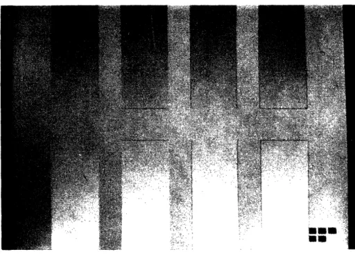
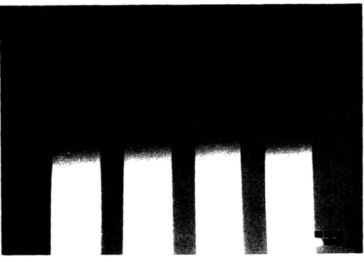
Consider Figures 1.3 and 1.4. In each figure, there is a set of four vertical bars each possessing a zero contrast region about their centres. The difference between the two figures is that the slope of the luminance gradient on either side of the gap is much greater in Figure 1.3 than in Figure 1.4. With respect to the left-most bar in Figure 1.3, the gap between the upper and

lower portions of the bar is clearly visible and there is little or no tendency to experience a continuation of the vertical edges through the gap. By way of comparison, although the gap in the left-most bar in Figure 1.4, is detectable, there is an impression of a contour connecting the top and bottom portions of the bar. That is, the visual system is biased towards completing the vertical contours of the bar when the gap is bounded by smooth endings, and to not so complete when it is surrounded by more sudden endings.

The effect of other discontinuities on such completion is demonstrated by the remaining three bars in Figure 1.4. With respect to the second bar from the left, two straight edges have been added joining together the two pairs of vertical edges ending above and below the gap. The marking of the top and bottom of the gap in this way has the effect of making it more apparent; there is less of a tendency to perceive the vertical edges of the bar as extending across the gap. In the case of the third bar, the smoothness of the endings has been eliminated while retaining the luminance characteristics of the bar. Here, the abrupt endings on the left and right edges clearly inhibit any bias to perceive the bar as complete. Completely enclosing the top and bottom portions of the bar, as in the right-most bar in the figure, has a similar effect of making the gap clearly visible.

These examples lead to the following hypotheses regarding contour com-pletion. First, smooth endings increase the likelihood of the perception of a contour not defined by a luminance change in the image. That is, smooth endings are likely to induce interpolation between them. Abrupt endings, in contradistinction, lead to the perception of "gaps". Second, smooth end-ings will lead to completion only under the condition that there is no other discontinuities restricting their continuation. Other edges provide clues that suggest further extension of the edge segment is not warranted. Thus, even when smooth endings are present in the image, they should not lead to interpolation if there is an event otherwise marking the gap between the endings-the gap should be clearly visible. Finally, this latter prediction has as a corollary that a stimulus which is in fact complete will be seen as gapped if there is information implying that there is a gap in the stimulus.2

20bviously, this latter prediction will hold only when the edge is of low contrast; high contrast edges are detectable no matter what else is present in the image.

1.3

Plan of the Thesis

These hypotheses were tested using two different paradigms and the results are reported, in detail, in the following chapters. They are described briefly here.

First, a detection task was used to determine whether subjects perceived contours when there was no luminance change in the stimulus. Subjects were presented with stimuli like those of Figures 1.4 and 1.3 and were required to judge whether there was a gap in the central region of the stimulus. The ra-tionale behind this set of experiments was that any tendency to complete the contour should reflect in subjects' judgments-they should report "gaps" less often when the stimulus figure was designed to increase the likelihood of in-terpolation. The results confirmed the hypotheses. Stimuli involving smooth edge endings were judged "gapped" less often than those with abrupt end-ings. Also, "gapped" judgments were modified according to the presence or absence of various discontinuities. In general, the addition of any "news" increased the likelihood that a gap was perceived. In terms of ranking the effectiveness of the cues, a "box" drawn around the top and bottom of the stimulus induced the greatest number of "gapped" judgments, followed by abruptly ending vertical edges and, lastly, horizontal edges (see Figure 1.4). Furthermore, the presence of these cues caused the perception of a gap even when the stimulus was actually complete. This occurred when a low con-trast but superthreshold edge was present in the "gapped region". These experiments are reported in Chapter 2.

Indirect evidence for completion is reported in Chapter 3. In a second set of experiments, the functional similarity between interpolated and real edges was assessed using the Poggendorff Illusion. To the extent that a gap causes an effect similar to that induced by real edges, here a Poggendorff Illusion, it can be concluded that the gap is not perceived as such; rather, at some level of processing within the visual system, the gap is filled in.

The results corroborated those reported in Chapter 2, although they were not as straightforward. To a first approximation, regions of physically zero contrast produced a significantly greater Poggendorff Illusion when bounded by smoothly ending edges as compared to those which ended abruptly. The gaps in the former stimuli did not behave like gaps, but as if a contour had been interpolated across the gap.

creased; and, when the difference was zero, no effects were observed. It appears that a gap bounded by abrupt endings did not induce a Poggendorff Illusion but induced a similar kind of effect based on the relationship between the shape of the gap and the rest of the stimulus figure.

The results of these two sets of studies are reported hereafter. In Chap-ter 4, the findings are discussed in the context of other related psychophysical phenomena including subjective contours, grating induction (McCourt, 1982), and phantom contours (Tynan & Sekuler, 1975). Also, the relationship be-tween contour completion and edge detection algorithms is considered.

Chapter 2

Detection Experiments

The first set of experiments employed a gap detection task to test the hypoth-esis that smooth edge endings are likely to induce contour completion, and abrupt endings are not. Subjects were asked to view a number of stimulus figures and simply report whether a particular stimulus appeared to possess an area of zero contrast, or "gap", at its centre. Subjects were required to judge (a) if a single stimulus possessed a gap (Experiments 2.2 and 2.3), or

(b) which of a pair of stimuli possessed a gap (Experiments 2.4 and 2.5). The stimuli were varied in ways that, according to the hypotheses dis-cussed in the previous chapter, increased or decreased the probability that subjects would perceive a gap. One of the variables studied was the slope of the luminance gradient on either side of a region of zero contrast. It was pre-dicted that a gap would be seen more often when the gradient was relatively steep. Figures 2.1 and 2.2 illustrate this factor.

If contours are interpolated when continuity is implied by the ending, then if the continuity can be counteracted, interpolation should be checked. A second manipulation of the displays was the introduction of discontinu-ities whose purpose was to enhance gap detection. Faint edges, which are discontinuities in luminance, were used. These were placed near the gap in order to inhibit contour interpolation across the gap. These discontinuites constituted cues to the presence of the gap.

Four types of cues were used and these are illustrated in Figure 2.1. There is no cue marking the zero contrast area of the left-most stimulus, and it was predicted that this type of stimulus would be judged "gapped" the least. In this case, the edges ended smoothly on either side of the gap,

the edge segments at the top and bottom of the zero contrast region. The second type of cue consisted of the placement of vertical lines that coincided with the vertical edges of the stimulus figure. These lines ended abruptly at the top and bottom of the gap. In this case, the edge segments did not end smoothly and it was predicted that this type of cue would also increase the perceptibility of the gap. The third cue consisted of a combination of the previous two, forming a "box" around the top and bottom of the stimulus, and it was expected that this too would enhance gap detection.

The hypothesis that cues enhance gap detection has as a corollary that a gap should be seen even when there is none in the stimulus. To test this, stimuli like those shown in Figure 2.3 were used to determine if subjects could be fooled into detecting non-existent gaps. The contrast of the vertical edges of these "complete" bars is low about their centres. It was predicted that since these edges were of low detectability, the cues would modify subjects' judgments and increase the frequency with which "gaps" were detected.

There was some concern that subjects would behave like a photometer given this kind of task. By asking subjects directly whether or not a par-ticular stimulus has a gap, they are thereby informed that there may not actually be a gap in the stimulus and that, thus, they should adopt a fairly strict criterion. They will tend to look closely at each stimulus and examine it for any indication that it has a gap. This could lead to the uninteresting result that they could detect the gap almost 100 per cent of the time, and the results would say nothing about smooth vs. abrupt endings, nor the ef-fects of the cues. In order to restrict such behaviour, therefore, stimuli were presented for a brief duration, and on occasion followed by a mask, so that the subjects could rely only upon their first impression of the stimulus.

Use of a brief presentation time gave rise to a concern that the low contrast edges of the complete stimuli (Figure 2.3) would be undetectable. If the con-trast of these edges was subthreshold, then there is no reason to suspect that the cues account for any increase in the number of "gapped" judgments-the subjects would not see judgments-these edges even if cues were absent. Therefore, a group of subjects was run in a standard contrast threshold study in order to establish the minimum detectable contrast, and thereby insure that any results obtained with the complete stimuli were not due to the invisibility of

Experiment 2.1

Method

Subjects. Eight University of Western Ontario undergraduate students

took part in the study to fulfill a course requirement. Seven of the students were 19 years of age, the remaining one was 18. Five were male and three were female. All had normal or corrected to normal vision.

Apparatus and Stimuli. The following apparatus was used in all of the

experiments. Stimuli were produced using a Matrox graphics system, con-sisting of two RGB-Graph/64-4 boards and a VAF-512/8 board. This system produced a display area 512 pixels wide by 480 pixels high. Given the view-ing distance of 98.7cm, each pixel subtended 1.69' of visual angle horizontally by 1.35' vertically. The stimuli generated by this system were displayed on an Electrohome RGB monitor, model number 38-D013101-60. This appa-ratus was capable of producing 256 grey levels, ranging from 4.3 candelas ("black") to 233 candelas ("white"). A Volker-Craig VC4152 terminal was used to record subjects' responses. The experiments were computer run on a National Semiconductor 16032 minicomputer under the Unix operating system. A chin rest was used to stabilize subjects' heads.

The stimuli consisted of a single vertical bar 10.82 deg of visual angle high by 1.97 deg wide, displayed upon a larger background of constant luminance (97 candelas). The dimensions of the background were 10.82deg high by 14.42 deg wide. The bars were presented 1 deg to the right of a central fixation cross. The reason for this was that, in Experiments 2.4 and 2.5, a pair of bars were presented to the left and right side of fixation. It was desired that the detection thresholds estimated in the current study be obtained under similar conditions, in which sensitivity is potentially decreased by an off centre display.

The contrast of the bar varied from trial to trial. Contrast was calculated using the formula (Lbackground - Lba)/(Lbackground + Lbar). Contrast ranged

from zero per cent to a maximum of 4.41% darker than the background. On each trial, the stimulus bar was presented for a duration of 864 msec; an abrupt stimulus onset was used.

de-termine subjects' contrast thresholds. For one of the staircases, the stimulus contrast was set initially to zero per cent, and, for the other, to the max-imum contrast. Step size was a constant 1.5 candela increase or decrease of the bar's luminance (the resolution of the equipment). Criterion was set at eight turnarounds, where the last six of these were used to estimate the threshold. Wetherill's decision rule two (Carterette, 1984) was used to re-verse the direction of the staircase: Contrast was lowered only after subjects had indicated that they had seen the stimulus for two successive presenta-tions (within the same staircase); contrast was increased after a single failure to detect the bar. This procedure estimates the 70.71% threshold.

Procedure. In order to reduce reflection from the monitor screen, the

room lights were turned off at the beginning of the experimental session. Under these conditions, the room was not completely dark, only dim. While subjects were dark adapting, the procedure was explained to them. They were instructed to place their heads in the chin rest and to gaze at the fixation cross on the monitor screen. They were told that they would be presented with a number of vertical bars, slightly to the right of fixation, and that they were to indicate whether they had seen the bar or not. If they had, they were to press the "y" key on the terminal keyboard, the "n" key otherwise.

The sequence of events was then explained. At the beginning of each trial, the screen was set to the background luminance. During this time, the computer generated the display specific to the trial, but did not show it. The terminal beeped to indicate to the subject that the stimulus was ready for presentation. Subjects were told that they were to prepare themselves for its presentation, gaze at the fixation cross, and to press the space bar on the keyboard when they were ready. Shortly after pressing the space bar, the stimulus bar was presented and then erased. The appearance of the stimuli was of a bar flashed briefly against a constant grey background. The terminal beeped a second time to signal that the bar had been shown. Subjects were instructed to press the appropriate key at this point, indicating whether they had seen a bar during the interval between the first and second beep. After they had made their response, the computer proceeded to the next trial and the process was reiterated until the staircase criteria were met. The interval between trials was approximately 10 seconds.

Due to equipment failure, the stimulus was presented, on occasion, for longer than the desired interval, and remained on the screen for about four

repeated at later time. After all trials were completed, the subjects were given a short written account explaining the purpose of the study, and any questions that they had about the study were answered.

Results

For each subject, the thresholds estimated from the ascending and descending staircase were combined and a mean computed. The contrast threshold for each of the eight subjects was 0.35%, 0.79%, 0.4%, 0.85%, 0.4%, 1.24%, 0.52%, and 0.4%. The mean of these estimates is 0.62%. Given the luminance of the background used in the current experiment, the minimum contrast the apparatus was capable of generating was 0.7%, a value slightly higher than the obtained mean threshold. In other words, on average, the subjects could detect an edge possessing the minimum possible contrast.

The reason that the threshold is less than the minimum possible con-trast is a function of the manner in which the threshold is calculated. The threshold is estimated as situated somewhere between the minimum level of contrast at which subjects always" detect the bar, and the maximum level at which they "never" detect the stimulus. In this particular study, the two levels in question were the minimum possible contrast and zero contrast.

Experiment 2.2

The next two experiments measured the absolute detectability of gaps. Sub-jects were shown single bars and were asked to say whether the bar possessed

a gap. Later studies measured relative detectability by presenting subjects with pairs of bars.

Method

Subjects. Ten University of Western Ontario undergraduate summer

school students were paid $10 for their participation in the study. Their ages ranged from 19 to 29. Seven were female and three were male. All had

normal or corrected to normal vision. All were naive with respect to the purpose of the study.

Stimuli. There were ten displays each consisting of a single vertical bar

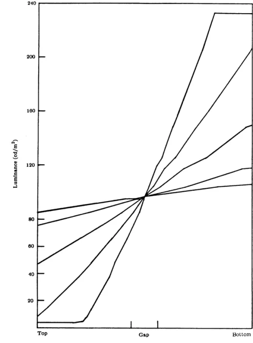
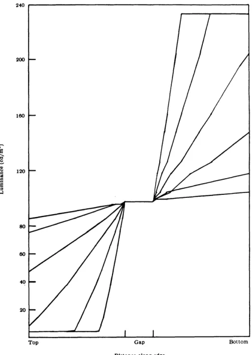
centred on the background. The luminance of the stimuli, and hence the contrast between them and the background, varied as a ramp function of the bar's height. Each bar was darker than the background at the top of the display, and became progressively lighter towards the bottom of the dis-play; bar luminance equalled the background luminance at the centre of the display. Five bars served as experimental stimuli and possessed a region of zero contrast about their centres, 1.35 deg of visual angle in height. That is, their luminance was constant and equal in value to that of the background beginning at a distance of 4.74 deg from the top of the display and ending at 6.09 deg. From here on, the luminance of the bar increased. These stimuli are referred to as "gapped".

The luminance of the five control stimuli did not likewise plateau, but continuously increased from the top to the bottom of the display. As such, these stimuli did possess a gap, albeit much smaller than that of the gapped bars (physically, one pixel or 1.35' in size). These latter five bars are termed "complete". The luminance profiles of the complete and gapped bars are il-lustrated in Figures 2.4 and 2.5, respectively. As can be seen in the figures, if the maximum ("white") or minimum ("black") luminance the apparatus was capable of generating was reached, the bar's luminance was set to "white" or "black" over its remaining length. The steepest gradient depicted in Fig-ure 2.5 was not used in the present study.

The bars varied in terms of the slope of their luminance profiles, which were approximately linear. The slope of the profile is reported here as:

gradient slope = AL/As

where AL is the change in luminance (in cd/m2) and As is the change in position along the height of the bar (in degrees of visual angle). Larger slopes denote steeper luminance gradients. For example, a step change in luminance (the steepest gradient possible) has a value of infinity, while no gradient is denoted by "zero"; the latter represents a situation in which there is no stimulus bar in the display. The slopes of the luminance gradients of the five complete bars were 1.96, 3.95, 9.45, 18.23, and 32.20 cd m- 2 deg- 1. The comparable slopes for the five gapped bars were 2.45, 4.47, 10.50, 18.72,

200 10 120 80 60 40 20

Top Gap Bottom

Distance along edge

Figure 2.4: Luminance profiles of the complete stimuli.

E .0I V U 2 E 0 L;1

and 31.87 cd m- 2 deg-'. The luminance gradients of the complete bars were selected such that their overall luminance matched that of their gapped coun-terpart. The luminance of the bars ranged from 85-104 candelas, 76-118 can-delas, 47-148 cancan-delas, 8-204 cancan-delas, and 4.3-233 cancan-delas, respectively, for each of the five pairs of complete and gapped bars.

Note that the five levels of gradient slope effectively changed the overall contrast of the stimulus bars. Bars with steeper gradients were of greater average contrast than those defined by shallower gradients. In particular, that area of the complete stimuli, corresponding to the zero contrast region of the gapped stimuli, varied in its average contrast. The mean contrast of this area was 0.88%, 1.05%, 1.40%, 4.90%, and 8.10%, respectively, for the five complete bars. Figure 2.3 shows the 1.05% contrast stimuli.

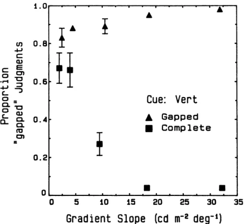
A second feature of the displays was the type of cue marking the top and bottom of the central region. Four cues were tested: (1) a no cue condition in which the stimulus bar appeared as described above, (2) a condition in which a pair of horizontal lines were placed at the top and bottom of the central region, connecting the left and right vertical edges of the bar, (3) four vertical lines collinear with the outer edges of the bar, each ending abruptly at the top and bottom of the central area, and (4) a combination of horizontal and vertical lines which formed a "box" around the top and bottom sections of the bar (see Figures 2.1 and 2.3). The cues were placed at the top and bottom of the gap in the case of the gapped bars, and, for the complete bars, at the same spatial locations as on the gapped bars.

The luminance of the cues was set so that they were slightly darker than the bar at the top and bottom of the central region. A constant decrease of 18 candelas was used. For the gapped stimuli, this meant that the luminance of the cue lines was consistently 78.57 candelas, since the luminance at the top and bottom of the gap was equal to the background. For the complete bars, the luminance of these lines varied since, here, the luminance at the top and bottom of the central region of the bar differed for each of the five stimuli. The luminance of the cues at the top were 76.86, 75.84, 72.42, 66.14, and 56.64 candelas, respectively. At the bottom, they were 80.55, 81.30, 85.40, 92.91, and 103.16 candelas, respectively.

All 40 displays were shown to each subject. Subjects were run in two blocks of 200 trials each; within each block, each display was presented on five separate occasions. Thus, each subject made a total of 10 judgments

200 160 4" 120 E 80 60 40 20

Top Gap Botto

Distance along edge

Figure 2.5: Luminance profiles of the gapped stimuli.

per display. The order of presentation of the various displays was random-ized for each subject and for each of the two blocks of trials. Each display was presented for a duration of 864 msec followed by a "white" mask (233 candelas); an abrupt stimulus onset was used. Seven displays were used for demonstration purposes; these consisted of some of the displays described above, as well as others of similar construction.

Procedure. Lighting conditions were dim, as before. Subjects were shown

the first example display, an no-cue gapped bar with a contrast gradient of 31.88 cd m- 2deg-l. The gap was readily visible in this display. Subjects were told that they were going to view many similar figures and that their task was to judge whether the bar had a gap in its vertical centre. It was emphasized that if the bar did possess a gap, then that gap would be always centrally located and equivalent in size to that shown in the example. The second example display was then shown, a no-cue gapped bar with a gradient of 4.47 cd m- 2_{deg-'. Subjects were told that the gap was not always as}

easily detected as that in the first display. This second display illustrated that point. The third example display was then shown, which consisted of a no-cue complete bar with a gradient of 9.45 cd m- 2_deg-1_{. This display was}

used to exhibit the appearance of a complete bar with a shallow luminance gradient, that sometimes the vertical edges in the central region would be difficult to see even though there was no gap in the stimulus. Finally, a gapped bar with a gradient of 10.49 cd m- 2_{deg-' and the horizontal lines}

cue was shown. Here subjects were told that, in addition to the bars, there frequently would be various faint lines near the central area of the bar. It was emphasized that these lines would be displayed regardless of whether the bar had a gap or not, and that the lines might help or might hinder them in their task. They were instructed to decide whether the stimulus did indeed possess a gap, to the best of their ability. During this phase of the experiment, the displays were not flashed briefly, but were shown for longer durations so that the subjects could inspect the figures and see them clearly. The mechanics of the experiment were then explained to the subjects. At the beginning of each trial, the monitor screen was black and remained so while the computer generated the next display to be shown. When the display was ready, the terminal beeped as a signal to the subjects. Subjects were told that when they were prepared to view the display, they were to press the space bar on the terminal any time after the beep. They were advised that it was best to look approximately at the centre of the monitor screen before

U, 0.8 4-J c 0) c E cm0.6 L C. C 0.4 SC 0.2 0 0 5 10 15 20 25 30 35

Gradient Slope

(cd m

2

_deg

- ')

Figure 2.6: Proportion "gapped" judgments as a function of gradient slope, no cue (Experiment 2.2).

pressing the space bar (no fixation cross was provided in the current study). Shortly after pressing the space bar, the display was presented, followed by the mask. Subjects were instructed to press the y" key on the terminal if they thought the stimulus bar did possess a gap, or the "n" key if they felt it did not possess a gap. They were told to guess if necessary. After pressing one of these keys, the monitor screen went blank, and the procedure reiterated.

The subjects were then run in a block of eight practice trials in order to familiarize them with the equipment and procedure. Following the practice trials, the subjects were run through the first block of experimental trials. There then followed a short break of approximately five minutes followed by the second block of experimental trials. As in the previous experiment, the stimulus occasionally was presented for a longer period than desired. The

I

I

Cue: None

.

·

,

, , .

.

.

, .

,

,

trials on which this happened were noted, and these trials were repeated at the end of the block in which they occurred. After all trials were completed, the subjects were suitably debriefed.

Results

The proportion of "gapped" judgments made by each subject for each display was calculated. The mean proportion "gapped" judgments collapsed over all subjects are shown in Figures 2.6-2.9. The slope of the contrast gradient is given on the x-axis and the proportion "gapped" judgments on the y-axis. Triangles represent judgments made in conjunction with bars that were truly gapped; squares represent responses made when presented with complete bars.

For gapped bars, it is obvious that the steeper the gradient, the more likely subjects were to judge the bar as possessing a gap. Subjects' performance was near perfect for the steepest gradient, and inspection of Figures 2.6 through 2.9 reveals than the type of cue had little effect in this case. The gap was clearly detectable when the contrast gradient was steepest.

For shallower luminance profiles, subjects were less inclined to make a "gapped" judgment, and here their judgments were influenced by the type of cue surrounding the gap. They were least likely to judge a stimulus as gapped if there was no cue to its existence, and increasingly more likely to so judge as the type of cue changed from horizontal lines, to vertical lines, to a box.

Since the means and variances of this data are not independent, individual subjects' proportions were transformed according to the arcsin transforma-tion (Kirk, 1968), and these transformed scores were analyzed according to a five (gradients) by four (cues) analysis of variance with repeated measures on both factors. There was a main effect of gradient slope, F(4, 36) = 24.02, p < .001, and a main effect of cue, F(3,27) = 15.87,p < .001. There was also a significant interaction between the slope of the gradient and the type of cue, F(12,108) = 4.63,p < .001. The interaction indicates that the zero contrast region was most apparent when the luminance gradient was steep, and that subjects could easily perceive it in this condition regardless of any enhancement provided by the cues. Indeed, the cue was superfluous when the gap was already so clearly defined. When the gap was not as distinct, the type of cue was a factor in terms of increasing the number of "gapped"

cn 0.8 c o E o_ 0.6 003 O_ X = 0.4 o 0.2 0 0 5 10 15 20 25 30 35

Gradient Slope (cd m

- 2

_deg

- ')

Figure 2.7: Proportion "gapped" judgments as a function of gradient slope, horizontal lines (Experiment 2.2).

judgments. Different cues were more influential than others.

A complementary pattern of results was obtained with complete bars. As can be seen in Figures 2.6-2.9, the proportion "gapped" judgments became less as the slope of the luminance gradient increased. The subjects were virtually perfect when the gradient was steep, and made more errors as the slope became less steep. Inspection of Figures 2.6 through 2.9 reveals that, for shallow contrast gradients, the proportion of "gapped" judgments increases as the cue went from none, to horizontal lines, to vertical lines, to the box, increasing by as much as 29%.

Proportions were again transformed and analyzed according to a five by four repeated measures analysis of variance. The results paralleled those ob-tained using gapped stimuli. Both main effects were significant, (F(4, 36) =

69.82,p < .001, and F(3,27) = 12.74,p < .001, respectively) as well as the

I

ii

I

Cue: Horiz

l

I

. T~~~~~

1.U m 0.8 C CE oo C 0) U 0.2 0 0 5 10 15 20 25 30 35

Gradient Slope (cd m

_deg

Figure 2.8: Proportion "gapped" judgments as a function of gradient slope, vertical lines (Experiment 2.2).

interaction, F(12, 108) = 5.75,p < .001.

The results are summarized as follows: First, when the zero contrast re-gion was clearly visible, or alternatively clearly absent, then the subjects perceived the stimuli accurately and made their judgments in accordance with their perception. In this case, the presence of various cues had no influ-ence on the perception of the central region. Second, when the central region was not clearly defined in terms of whether it possessed an actual gap or a faint edge, then subjects made more errors, judging gapped stimuli as com-plete and comcom-plete bars as gapped. Third, their judgments for the shallow gradient stimuli were influenced by the type of cue. It appears that there being no cue in the display was most conducive to incurring a "complete" judgment. The addition of any cue increased the proportion of "gapped" judgments. For the different cues, horizontal lines had a lesser effect than

Cue: Vert

A

I Complete

'....U - U

-4-c E

*.

Gradient Slope (cd

m

_deg

_')

Figure 2.9: Proportion "gapped" judgments as a function of gradient slope, box (Experiment 2.2).

either vertical lines or a box. The latter two cues induced approximately equal proportions of "gapped" judgments. These results indicate that when edges are difficult to see, subjects relied on other information in the stimulus to determine whether there really was a gap in the bar.

Experiment 2.3

Experiment 2.3 replicated the previous study using bars defined by reversing gradients. That is, the bars were defined by gradients of increasing luminance from the top of the display to the centre, then decreasing luminance over the rest of their length. The luminance of the bars in the previous experiment increased over their entire length (see Figures 2.4 and 2.5). The result of designing the stimuli in this manner was that the contrast of the central

Cue: Box

I

l1 * Ga Completee

region of the complete stimuli was constant over its length.

Method

Subjects. Ten first year undergraduate University of Western Ontario

students participated in the study to fulfill a course requirement. Their ages ranged from 19 to 27. Seven were female and three were male. All had normal or corrected to normal vision. None had participated in previous experiments.

Stimuli. The stimuli were similar to those of the previous experiment,

with the following differences. Three bars were used, whose luminance pro-files were again a ramp function of the height of the bar. The slope of the gradient was equal to 4.47 cd m- 2 _deg- 1 _{for all three bars; however, in the}

present experiment, the direction of the gradient reversed at the centre of the bar. That is, as before, the bars were darker at the top of the screen and became progressively lighter in luminance towards the centre of the display. The luminance of the bar did not continue to increase upon reaching the bot-tom of the central region, but decreased in luminance towards the botbot-tom of the screen. In short, the intensity profile of the bottom half of the bars was a mirror image of their top halves.

The luminance of a region 1.35 deg about the centre of the bars was held constant, and the three bars differed with respect to the contrast of this region. In one case, the luminance of the central region was set to that of the background, resulting in a gap of zero contrast. For the second bar, the contrast between this region and the background was set to 0.88%, and the third was 2.8%. These contrasts were obtained by decreasing the intensity of the first bar everywhere by a constant amount. There was thus an gapped bar, a complete bar with a relatively faint edge through its centre, and a complete bar with a stronger edge. The three luminance profiles were crossed with the four types of cues. The cue lines were a constant 18 candelas darker than the luminance of the bar at the top and bottom of the central region. An example is shown in Figure 2.10; here the gapped bar.

Each of the 12 displays was presented on 10 occasions resulting in a block of 120 trials. Each subject received a different random order of the trials. In the current study, stimulus onset was abrupt, preceded and followed by an blank screen equal in luminance to that of the background.

1.U ') -.- 0.8 c o E CL c 0.6 C C0 0. 0.4 0.2 0

7

;/

/

/

/~

/

/

7

/

/

/

/

/

/

/

/

/

/

/

/

/

/

_/

/

/

/

/

/

_/

_L

/1

K

K

Contrast

at Centre:

0o.o%

-- 1 . 88%

3

2.8%

None

Horiz

Vert

Box

Cue

Figure 2.11: Proportion "gapped" judgments as a function of cue type (Ex-periment 2.3).

2.2, with the following differences. A different set of demonstration/practice displays was used in order to match the reversing luminance profiles of the displays used in the experiment proper.

The sequence of an individual trial differed slightly from that in Experi-ment 2.2. At the beginning of the trial, before the terminal beeped, monitor screen luminance was identical to that of the background of the displays. When the subject initiated a trial, this field was replaced by the particular stimulus for that trial, which was subsequently erased. The appearance of the stimuli was that of a bar flashed briefly against a grey background.

Results

The proportion of "gapped" judgments made by each subject for each display was calculated. The means are shown in Figure 2.11. The type of cue is labelled on the x-axis, and the proportion "gapped" judgments on the y-axis.

1