Maximizing noise energy for noise-masking studies

HAL Id: hal-01375454

https://hal.sorbonne-universite.fr/hal-01375454

Submitted on 3 Oct 2016

HAL is a multi-disciplinary open access archive for the deposit and dissemination of sci-entific research documents, whether they are pub-lished or not. The documents may come from teaching and research institutions in France or abroad, or from public or private research centers.

L’archive ouverte pluridisciplinaire HAL, est destinée au dépôt et à la diffusion de documents scientifiques de niveau recherche, publiés ou non, émanant des établissements d’enseignement et de recherche français ou étrangers, des laboratoires publics ou privés.

Maximizing noise energy for noise-masking studies

Cédric Jules Étienne, Angelo Arleo, Rémy Allard

To cite this version:

Cédric Jules Étienne, Angelo Arleo, Rémy Allard. Maximizing noise energy for noise-masking studies. Behavior Research Methods, Psychonomic Society, Inc, 2016, pp.1-13. �10.3758/s13428-016-0786-1�. �hal-01375454�

Maximizing noise energy for noise-masking studies

1_{Sorbonne Universités, UPMC Univ Paris 06, INSERM, CNRS, Institut de la Vision, Paris, France}

http://www.aging-vision-action.fr

Corresponding author: Rémy Allard Address: 17 rue Moreau, Paris, France, 75012

Telephone number: 011 33 (0)1 53 46 26 55

Abstract

Noise-masking experiments are widely used to investigate visual functions. To be useful, noise generally needs to be strong enough to noticeably impair performance, but under some conditions, noise does not impair performance even when its contrast approaches the maximal displayable limit of 100%. To extend the usefulness of noise-masking paradigms over a wider range of conditions, the present study developed a noise with great masking strength. There are two typical ways of increasing masking strength without exceeding the limited contrast range: use binary noise instead of Gaussian noise or filter out frequencies that are not relevant to the task (i.e., which can be removed without affecting performance). The present study combined these two approaches to further increase masking strength. We show that binarizing the noise after the filtering process substantially increases the energy at frequencies within the pass-band of the filter given equated total contrast ranges. A validation experiment showed that similar performances were obtained using binarized-filtered noise and filtered noise (given equated noise energy at the frequencies within the pass-band) suggesting that the binarization operation, which substantially reduced the contrast range, had no significant impact on performance. We conclude that binarized-filtered noise (and more generally, truncated-filtered noise) can substantially increase the energy of the noise at frequencies within the pass-band. Thus, given a limited contrast range, binarized-filtered noise can display higher energy levels than Gaussian noise and thereby widen the range of conditions over which noise-masking paradigms can be useful.

Keywords

Introduction

Noise-masking experiments are widely used to investigate visual functions (Allard, Faubert, & Pelli, 2015; Lu & Dosher, 2008; Pelli & Farell, 1999; Pelli, 1981). Masking occurs when the noise noticeably impairs the observer’s performance, but under some conditions,

performance remains unaffected even when the noise approaches 100% contrast. For instance, consider using a noise-masking paradigm to investigate the internal factors limiting contrast sensitivity (e.g., Pelli & Farell, 1999). The noise energy required to noticeably impair the detection threshold is minimal at middle spatial frequencies and gradually increases at low and high spatial frequencies. At low spatial frequencies, the impact of noise is attenuated by sparser and larger receptive fields integrating (~averaging) the noise over large areas and thereby weakening its masking strength (Raghavan, 1995). At high spatial frequencies, the impact of the noise is attenuated by the modulation transfer function of the eye reducing the effective contrast of the stimulus (Campbell & Gubisch, 1966) and therefore requiring high noise energy to noticeably impair performance. As a result, the frequency range over which noise can effectively impair performance is limited by the maximal external noise energy that can be displayed, that is, without exceeding 100% contrast. Furthermore, the noise energy required to impair detection also increases when reducing luminance intensities, especially at high spatial frequencies (Raghavan, 1995). Displaying more noise energy would widen the frequency and luminance range over which noise-masking paradigms could be implemented. To extend the usefulness of noise-masking paradigms, the present study developed a new noise maximizing the displayable energy.

Many noise-masking paradigms assume, usually implicitly, that the same underlying processing strategy operates in absence and presence of noise. But recent studies by Allard and colleagues (Allard & Cavanagh, 2011; Allard & Faubert, 2013, 2014a, 2014b; Allard, Renaud, Molinatti, & Faubert, 2013) suggested that this noise-invariant processing

assumption can be violated when using some types of noise. For instance, contrast detection is known to be immune to crowding, but adding noise that is spatiotemporally localized to the target (i.e., at the potential target locations and turn on and off with target) made a detection task vulnerable to crowding, whereas noise that is spatiotemporally extended (i.e., full-screen, continuously displayed dynamic noise) did not (Allard & Cavanagh, 2011). These results suggest that the processing strategy in localized noise involved processes vulnerable to crowding, whereas the processing strategy in absence of noise and in extended noise did not. The aim of the present study was to increase the noise-masking strength without triggering a change in processing strategy.

To avoid triggering a change in processing strategy, Allard and colleagues (Allard &

Cavanagh, 2011; Allard & Faubert, 2013, 2014a, 2014b; Allard et al., 2013) recommended to use full-screen, continuously displayed, dynamic noise. Unfortunately, using dynamic noise resampled at a high temporal rate instead of static noise tends to reduce the masking strength of noise due to temporal integration (i.e., averaging) occurring early in the visual system. The use of dynamic noise can therefore reduce the range of conditions over which noise-masking paradigms can be usefully implemented (i.e., noticeably impair performance). The constraint of using dynamic noise further emphasizes the need to maximize the displayable noise energy.

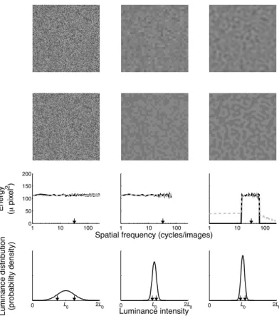
The standard way of adding visual noise to a stimulus is to introduce luminance variance to each pixel of the display, that is, to add a random luminance value drawn from a Gaussian distribution centered on 0 (left image of the top row of Figure 1) (Pelli, 1981). Given that the samples are not correlated between each other, such noise is white (flat energy spectrum, black curve in the left graph of the third row of Figure 1). This standard noise is typically referred to as “Gaussian noise”. For pixel white noise, the expected energy at all frequencies (e) can be defined as (Pelli, 1981):

𝑒 = 𝑉𝑎𝑟𝑖𝑎𝑛𝑐𝑒 𝑁 ∙ 𝑤 ∙ ℎ ∙ 𝑑 (1)

where Variance(N) represents the luminance variance across the samples within the noise matrix N (for samples drawn from a Gaussian distribution with standard deviation σ, the variance is equal to σ2), and w, h and d represent the width, height and duration of each noise pixel, respectively. Thus, the noise energy is proportional to the variance of the noise (i.e., squared contrast).

Figure 1. Different types of noise (first two top rows) and their corresponding spectral energy

distributions (third row) and luminance distributions (bottom row). The first row presents samples of Gaussian noise (left), low-resolution Gaussian noise (center) and filtered noise (right). The second row presents the binarized noises of the first row, namely, binary noise, low-resolution binary noise and binarized-filtered noise, respectively. The energy levels at the relevant frequency were equated across all 6 noises by scaling the noise contrast. See Movie 1 in supplementary material for dynamic noise. The third row represents spectral energy density of the different types of noise. The black solid lines represent Gaussian noise (corresponding images in first row), the grey dashed lines represent the binarized noise (corresponding images in second row) and the arrow represents the relevant (e.g., signal) frequency. The

1 10 100 0 50 100 150 200 Energy _(µ pixel 2) 0 L₀ 2L₀

Luminance distribution (probability density)

1 10 100 Spatial frequency (cycles/images)

0 L₀ 2L₀ Luminance intensity

1 10 100

bottom row represents the luminance distribution of the samples of Gaussian noise (black line) and the

two arrows show the two luminance intensities of the binarized noise. L0 represents the mean background

luminance intensity.

A typical way to modify Gaussian noise to increase its effective masking power is to concentrate its energy to frequencies relevant to the processing of the stimulus (Pelli, 1981; Solomon & Pelli, 1994; Stromeyer & Julesz, 1972). Another method simply consists in sampling the noise from a binary distribution instead of Gaussian distribution (e.g., Allard et al., 2013). The present study combined these two approaches to further increase masking power.

Binary noise

The distribution that maximizes the noise energy given a limited contrast range is a binary distribution in which one of two values is randomly selected independently for each sample (left image in the second row of Figure 1). Given no correlation across samples, binary noise is white (flat energy spectrum) and its energy can also be defined by Equation (1). Thus, binary noise has the same expected energy level at all frequencies as Gaussian noise given the same variance (left graph in third row of Figure 1). The variance of binary noise is equal to the variance of Gaussian noise (σ2) when the two values from which the samples are drawn are ±σ (left graph in bottom row of Figure 1).

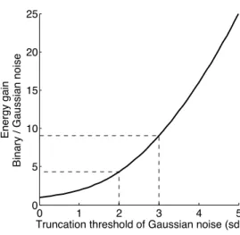
An advantage of a binary distribution over a Gaussian distribution is that the contrast range is finite and well defined. Theoretically, a Gaussian distribution extends over an infinite range (left graph in bottom row of Figure 1). Under experimental conditions, however, Gaussian noise is often truncated at 2 or 3 standard deviations (sd). Truncating at ±3 sd has little impact on the noise energy (0.5% reduction) as few samples fall outside this range. Truncating at ±2 sd still roughly preserves the shape of the Gaussian distribution, but substantially reduces the

distribution range while reducing the noise energy by only 8%. Given that truncated Gaussian noise has a finite and well-defined contrast range, its energy can be compared with the energy of binary noise given the same total contrast range (i.e., the two binary values set to the positive and negative truncation thresholds). As shown in Figure 2, the energy of binary noise is greater by a factor of 4.3 and 9.0 relative to the energy of Gaussian noise truncated to ±2 and ±3 sd, respectively.

Figure 2. Energy gain of using binary noise instead of truncated Gaussian noise as a function of the truncation threshold given equated total contrast ranges.

Non-white noise

For many experiments, the ideal noise would have a flat energy spectrum over all frequencies. However, to have the same energy level across an infinite range of frequencies, such an ideal noise would require infinitely small samples (e.g., w, h and d infinitely small) and its energy would therefore also be infinitely small for any finite sample variance (Pelli, 1981). In practice, a noise can have a flat energy spectrum over a finite range of frequencies and the maximal displayable noise energy can be increased by concentrating the noise energy over a narrower range of frequencies.

The simplest way of increasing the energy level is to decrease the spatial and/or temporal resolution of the display (e.g., center image in the top row of Figure 1 in which each noise

0 1 2 3 4 5 0 5 10 15 20 25

Truncation threshold of Gaussian noise (sd)

Energy gain

check size is set to 4x4 pixels rather than 1x1 pixels). For the same variance, reducing the resolution of the display increases the noise energy (Equation 1) and reduces the upper frequency limit of the noise (black curve in top center graph in Figure 1) so it can be used when the noise at these frequencies is not relevant to the task. Nevertheless, a drawback of low-resolution noise is that it introduces apparent edges between noise checks forming a grid as it can be seen in the center image in the top row of Figure 1. Because these apparent edges may have undesirable effects (e.g., Harmon & Julesz, 1973), it is safer to avoid them as their presence could potentially interfere with the processing of the target.

An alternative method that does not introduce artificial edges consists in filtering the noise to remove frequencies that are not relevant to the task (right image in the top row and black curve in the right graph in third row of Figure 1). Indeed, some frequencies can be removed to reduce the contrast range without affecting performance. For instance, removing the

frequencies outside ±1 octave from the spatial frequency of a sine-wave target does not affect detection threshold (Pelli, 1981; Stromeyer & Julesz, 1972). Filtering out information

irrelevant to the task (i.e., does not affect performance) is an efficient way of reducing the noise contrast (e.g., Gaussian distribution narrower for filtered noise compared to Gaussian noise, black curves in right and left graphs in bottom row of Figure 1, respectively). As a result, at equal contrast ranges, filtered noise would have higher energy at the frequencies within the pass-band.

Binarized-filtered noise

The rationale of the present study was to combine the two approaches described above (i.e., binary noise and non-white noise) to further increase the energy of the noise at the

frequencies relevant to the task. For low-resolution noise, the method simply consists in sampling noise elements from a binary distribution instead of a Gaussian distribution (center

images in top and second rows of Figure 1). Low-resolution binary noise is not novel as it has been used before (e.g., Allard et al., 2013). However, the drawback of using low-resolution noise remains: it artificially introduces apparent edges between noise checks. Alternatively, the present study combined binary noise with filtered noise (right image in second row of Figure 1). Binarizing the noise after the filtering operation substantially increases the energy level for equal contrast range. In other words, the binarized-filtered noise requires much less contrast than (unbinarized-)filtered noise to reach the same energy level at the frequencies within the pass-band (right graphs in third and bottom rows of Figure 1).

Binarizing filtered noise changes the profile of the spectral density function as it introduces energy at frequencies that were filtered out (e.g., right graph in third row of Figure 1). However, given that the energy at those frequencies is irrelevant (completely removing them should not affect performance), this small gain in energy should also be negligible for

masking experiments. More importantly, the binarizing operation does not affect the expected constant spectral density across the frequencies within the pass-band (right graph in third row of Figure 1).

Binarized-filtered noise requires less contrast than filtered noise to display the same expected energy at frequencies within the pass-band (right graph in bottom row of Figure 1). Thus, by equating the total contrast range, the binarized-filtered noise would display more energy at the frequencies within the pass-band than the filtered noise. To illustrate this energy gain, the energy level at frequencies within the pass-band of binarized-filtered noise was compared with the one of filtered noise (filtered 1 octave below and above a given spatial frequency) given equated total contrast range. As for Gaussian noise, the distribution of the samples of filtered noise also follows a Gaussian distribution theoretically extending over a wide contrast range (curves of left and right graphs in bottom row of Figure 1). Filtered noise was therefore truncated so that it had a finite and well-defined contrast range. Figure 3 compares the energy

at the frequencies within the pass-band of binarized-filtered noise with the truncated-filtered noise as a function of the truncation threshold given equated contrast range (i.e., the two binary values set to the positive and negative truncation thresholds). In this particular case, binarizing the noise and equating noise contrast was found to increase the noise energy by a factor of 3.3 and 6.7 when the filtered noise was truncated at ±2 and ±3 sd of its filtered distribution, respectively. This illustrates that binarizing filtered noise substantially increases the energy at the frequencies within the pass-band of filtered noise given equated contrast range.

Figure 3. Energy gain at frequencies within the pass-band when using binarized-filtered noise instead of truncated-filtered noise as a function of the truncation threshold given equated total contrast ranges. The filter was 2-octave wide in the spatial frequency domain.

Experiment: Binarized-filtered noise vs Gaussian noise

expected energy at the frequencies relevant to the task so both noises are expected to have the same masking strength. The main aim of this experiment was to empirically verify this prediction. If the performance in binarized-filtered noise differs from the one in Gaussian noise (given equated energy levels at frequencies within the pass-band), then the binarized-filtered noise cannot be considered equivalent to the Gaussian noise. On the other hand, if

0 1 2 3 4 5 0 5 10 15 20 25

Truncation threshold of filtered noise (sd)

Energy gain

Binarized

−

binarized-filtered noise has the same expected noise energy at the frequencies relevant to the task as Gaussian noise and has the same masking strength, then binarized-filtered noise can be considered as equivalent to Gaussian noise.

Method

Observers

Four naïve observers and one of the authors participated in this study. They had normal or corrected-to-normal vision.

Apparatus

Stimuli were presented on a 22.5-inch LCD monitor designed for psychophysics (VIEWPixx) with a refresh rate of 120 Hz. At the viewing distance of 1 m, the spatial resolution of the display was 64 pixels/degree of visual angle. The monitor was the only source of light in the room. The output intensity of each color gun was linearized psychophysically using a homemade program.

Stimuli and procedure

The detection task was implemented using a two-interval forced-choice procedure with an interstimulus interval of 500 msec. The noise was continuously displayed, refreshed at every frame and covered the entire screen. The signal was a 4 cycles-per-degree vertical grating presented in only one of the two 500-msec intervals. The spatial window of the signal had a diameter of 1 degrees plus a half-cosine soft edge of 0.25 degrees. A 500-msec sound was audible during each of the two intervals and the task consisted in determining if the target was present at the during the first or second sound by pressing one of two keys.

Two types of noise were used: filtered noise and binarized-filtered noise. For each noise type, the width of the ideal filter was 0.25, 0.5, 1, 2 or ∞ (i.e., unfiltered) octaves above and below

the signal spatial frequency of 4 cycles-per-degree, resulting in 10 conditions (2 noise types X 5 filter widths, Figure 4). In all the conditions, the expected energy levels at the unfiltered frequency were equated to 0.22 µ degree2 second.

Figure 4. The top left represents Gaussian white noise. The 2nd to the last column of the top row represents the same noise sample after applying a filter with a width of 4, 2, 1 and 0.5 octaves, respectively, centered on a given spatial frequency (here 16 cycles per image). Each noise at the bottom row represents the same noise sample as its corresponding top row, except that it was binarized and its energy at the frequencies within the pass-band was equated. See Movie 2 in supplementary material to for dynamic noise.

Contrast thresholds were measured using a 3down1up staircase procedure (Levitt, 1971) with step size of 0.1 log and was interrupted after 12 inversions. Threshold estimation of a

staircase was set as the geometric mean of the last 8 inversions. The 10 conditions were blocked and performed in a pseudo-random order. Each staircase was performed 5 times so that each threshold was set as the geometric mean of the 5 staircases.

Results and discussion

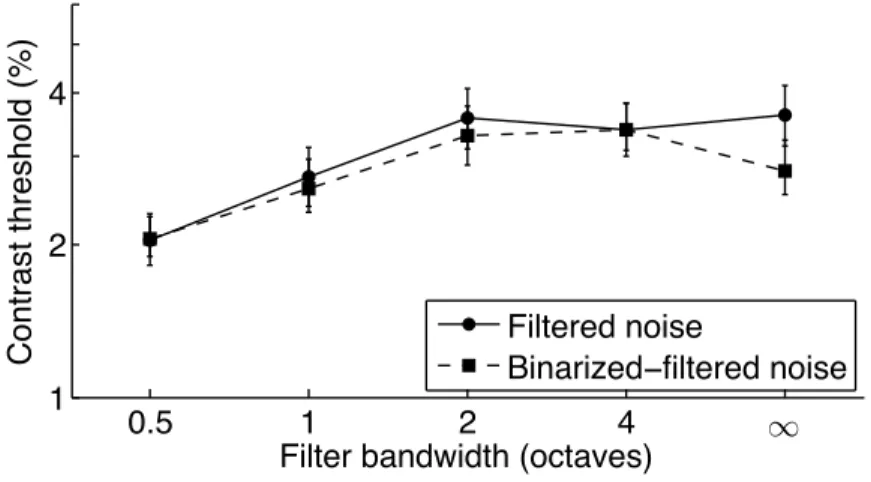
The results shown in Figure 5 illustrate the two main outcomes. Most importantly, similar contrast thresholds were obtained for filtered noise and binarized-filtered noise suggesting that binarization had no significant impact on the masking strength (given equated noise energy at frequencies with the pass-band as illustrated in right graph in third row of Figure 1).

bandwidths) that showed no simple main effect of noise type (F(1,16)=1.22, p=.332). Thus, binarizing the noise had no significant impact on performance even though it substantially reduced the noise contrast. This suggests that binarizing the noise can be used to reduce the contrast range of the noise without affecting performance.

Figure 5. Contrast detection threshold as a function of filter bandwidth centered on the spatial frequency of the signal obtained in filtered (circles) and binarized-filtered (squares) noises. Error bars represent standard error of the mean.

The second important outcome was that the filtering operation had no impact when the filter bandwidth was at least 2 octaves (Figure 5), that is, 1 octave above and below the signal spatial frequency, which is consistent with previous findings (Pelli, 1981; Stromeyer & Julesz, 1972). Note that statistically, the two-way ANOVA showed a simple main effect of filter bandwidth (F(4,16)=46.4, p<.001), which can be explained by the lower contrast thresholds when many frequencies were filtering out (e.g., <2 octaves bandwidth filters). Nevertheless, when measuring contrast detection threshold in noise, the same performance was observed whether the noise was white or had energy only 1 octave above and below the spatial frequency of the target. This suggests that, for a contrast detection task, removing the noise outside this frequency range reduces the contrast range of the noise without affecting performance.

1 2 4

Filter bandwidth (octaves)

Contrast threshold (%)

0.5 1 2 4 _∞

Filtered noise

Taken together, these two outcomes suggest that binarized-filtered noise at ±1 octave around the signal frequency was equivalent to Gaussian noise. Given that the filtering and binarizing operations substantially reduced the noise contrast range without affecting performance (given equated noise energy at frequencies within the pass-band), increasing the contrast of binarized-filtered would display higher noise energy at the relevant frequencies.

Truncated-filtered noise

The advantage of binarized-filtered noise is that it uses a narrower contrast range than Gaussian noise for a given masking strength, which enables to display higher noise energy (by increasing noise contrast). A potential issue with this noise is that the use of only two luminance intensities introduces sharp edges (e.g., Figure 1, bottom right). Because the position of these edges randomly varies over time, they are less salient than the edges for the low-resolution noises presented above (e.g., see Movie 1 in supplementary material).

Although these edges could potentially have an undesirable effect, the experiment above rather suggests that these edges had a negligible impact for this contrast detection task. Nevertheless, apparent edges could potentially cause binarized-filtered noise not to be equivalent to Gaussian noise. The present section shows that the visibility of these apparent edges can be substantially attenuated with the small cost of slightly decreasing noise energy (given equated noise contrast). Thus, even though the potential drawback of the binarization operation (i.e., introducing sharp edges) was empirically found to be negligible, the present section nevertheless shows that it can be substantially attenuated.

Above, to compare the energy of binary noise and Gaussian noise (Figure 2), the Gaussian noise was truncated at various truncation thresholds. Figure 2 shows that, for equated contrast ranges, the energy of truncated Gaussian noise approaches the one of binary noise as the truncation threshold approaches 0. This is because at an infinitely small truncation threshold,

truncated Gaussian noise is equivalent to binary noise. Thus, by varying the truncation value and equating the noise energy at frequencies within the pass-band, truncated Gaussian noise gradually varies from binary noise (truncation threshold = 0) to Gaussian noise (truncation threshold = ∞).

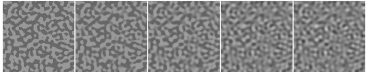
The same rationale applies to truncated-filtered noise (Figure 3), which gradually varies from binarized-filtered noise (truncation threshold = 0) to filtered noise (truncation threshold = ∞). Figure 6 shows truncated-filtered noise for different truncation thresholds (±0, 0.5, 1, 2 and ∞ sd). Note that the noise was truncated relative to the standard deviation of the noise after the filtering operation and not relative to the noise standard deviation of the initial Gaussian distribution used to generate the pre-filtered noise. Recall that the experiment above found the same performance whether binarized-filtered noise and filtered noise (i.e., truncated-filtered noises with a truncation threshold set to 0 and ∞, respectively). Given no performance

difference between these two extremes, there is no reason to expect a different performance at any intermediate truncation threshold when the expected energy at frequencies within the pass-band is equated. Thus, using truncated-filtered noise could be a good compromise between binarized-filtered noise, which introduces undesired edges, and filtered noise, which extends over a large contrast range.

Figure 6. Truncated-filtered noise with truncation threshold set to ±0, 0.5, 1, 2 and ∞ standard deviations (left to right). The expected noise energies at the relevant frequencies were equated. See Movie 3 in supplementary material for dynamic noise.

General discussion

By combining two methods of increasing noise energy given a limited contrast range (namely, filtered noise and binary noise), the present study developed a noise, namely truncated-filtered noise, equivalent to Gaussian noise with respect to a given task, but requiring less contrast to be displayed (see Appendix for detailed algorithm and Matlab code). Truncated-filtered noise was found to have the same masking strength as Gaussian noise when having the same expected energy at frequencies relevant to the task, which required less contrast. Thus, this new noise enables to display higher noise energy and thereby widen the range of conditions under which noise-masking paradigms can be effectively used. For instance, the amount of noise required to affect performance is known to gradually increase as luminance intensity is reduced (Pelli, 1981). To illustrate the usefulness of this method, we evaluated, for the same stimulus as in the experiment above, the lowest luminance intensity at which the maximal displayable noise could noticeably affect performance (i.e., increase detection threshold by a factor of at least 2). The lowest luminance intensities at which Gaussian, binary, filtered (±1 octave) and truncated-filtered (±1 octave, truncation=1 sd) noises could noticeably affect performance were found to be about 350, 39, 16 and 4 td, respectively. This simple example shows that truncated-filtered noise can be a useful tool to widen the range of conditions under which noise can be effectively be used. Note that maximizing noise energy could also be useful for other types of paradigms requiring strong masking, such as continuous flash suppression (Tsuchiya & Koch, 2005).

Truncated-filtered noise varies, depending on the truncation threshold, along a continuum between binarized-filtered noise (truncation threshold = 0) and filtered noise (truncation threshold = ∞, i.e., no truncation). Empirically, results showed that when equating energy at the frequencies relevant to the task, the same performance was observed for the two extreme

truncating the noise at any truncation threshold (while equating noise energy at frequencies within the pass-band) is a useful way of reducing the contrast range of the noise without affecting its masking strength.

The advantage of a low truncation threshold is that it reduces the contrast range required to display a given energy level. An apparent drawback is that it artificially introduces edges as for binarized-filtered noise (i.e., truncation threshold = 0, Figure 1). Truncating the noise at ±1 sd, was found, in the example above (center image of Figure 6), to substantially reduce the appearance of the edges and reduce the energy (given equated total contrast range) by a factor of only 1.4 relative to binarized-filtered noise. We can also note that using a truncation

threshold of ±2 sd compared to untruncated-filtered noise (fourth vs last image of Figure 6) has little impact on the noise appearance and provides the advantage of having a noise that covers a smaller and well-defined contrast range. However, a truncation threshold at ±2 sd reduced energy (given equated total contrast range) by about 2.8 times relative to binarized-filtered noise. Ultimately, choosing the truncation threshold depends on the experimental paradigm and its constraint (e.g., contrast available and potential issue of apparent edges), but the truncated-filtered noise at ±1 sd appears to be a good compromise, as it requires little additional contrast and substantially reduces the appearance of edges.

For truncated-filtered noise to be equivalent to Gaussian noise, they should have the same masking strength. The current study suggests that truncating (or even binarizing) filtered noise has no impact on performance given equated noise energy at frequencies within the pass-band (see Appendix for equating noise energy). Thus, truncated-filtered noise is equivalent to Gaussian noise, if the filtering operation has no impact on performance. In the current study, the noise was filtered according to the spatial frequency, but it could also be filtered along any other dimension such as temporal frequency or orientation. A priori, however, it is not possible to know what information can be filtered out without causing a

noticeable change in performance as it depends on which information is relevant to the visual system for the given task. The processing involved in a typical contrast detection task, for instance, is known to be narrowly tuned in the spatial frequency domain, which explains why a narrow filter (e.g., ±1 octave of the signal spatial frequency) has no effect on performance as observed here and elsewhere (Pelli, 1981; Stromeyer & Julesz, 1972). But for filtering along other dimensions, the filter that can be used without affecting performance depends on the tuning of the processing for the given task and cannot be known a priori. In sum, the filter that can be used to avoid reducing masking strength cannot be known a priori as it depends on the processing properties relevant to the given task. Obviously, truncated-filtered noise suffers from the same limitations as filtered noise. Nevertheless, once a filter is chosen (and assumed or shown not to have any impact on performance when applied to Gaussian noise), the current study suggests that the noise can be truncated in order to further increase energy and thereby extend the range of conditions over which noise-masking paradigms can be useful. See the Appendix for Matlab code to generate truncated-filtered noise filtered along the spatial frequency, orientation or/and temporal frequency dimensions.

A common use of external noise is to quantify the performance of human observers relative to the performance of an ideal observer (Gold, Abbey, Tjan, & Kersten, 2009; Kersten &

Mamassian, 2010). An ideal observer often has a perfect performance in noiseless condition (e.g., an infinitely small contrast detection threshold), but under noisy conditions, the optimal performance is limited even when using optimally all the available information. If the human performance is close to the ideal performance (e.g., Allard & Cavanagh, 2012; Allard & Faubert, 2013; Baldwin, Baker, & Hess, 2016), then this means that the observer efficiently integrates all the necessary information to perform the task. Otherwise, some information must be lost, deteriorated or not optimally integrated. Although truncated-filtered noise may be equivalent to Gaussian noise for a human observer, they may not be equivalent for an ideal

observer, which may use additional information only available in truncated-filtered noise (e.g., detect a signal when the luminance of any pixel exceed, even by an infinitely small amount, the contrast range of the truncated noise). Thus, at first sight, using truncated-filtered noise seems to compromise the comparison with the ideal observer even if truncated-filtered noise is equivalent to Gaussian noise for the human observer. However, a simple way to prevent the ideal observer from using additional information only available in truncated-filtered noise is to compare the human performance in truncated-truncated-filtered noise with the ideal performance in Gaussian noise. Indeed, given that the human performance in truncated-filtered noise is equivalent to the one in Gaussian noise, the human performance in Gaussian noise can be estimated and compared with the ideal performance. Thus, the use of truncated-filtered noise instead of Gaussian noise does not compromise the comparison with the ideal performance given that both noises are equivalent for human observers. Such a comparison can be performed by quantifying the noise energy of Gaussian and truncated-filtered noise at the unfiltered frequencies (see Appendix for a detailed algorithm and Matlab code).

The current method should not be confused with methods improving the contrast resolution of digital displays, such as the Noisy-bit (Allard & Faubert, 2008) or bit-stealing (Tyler, 1997) methods. These methods aim at overcoming practical limitations of the digital display (smallest contrast displayable), whereas the current study rather deals with the theoretical limit of 100% contrast displayable. Thus, these two kinds of method address distinct displayable contrast limitations (smallest and highest displayable contrast) and can be used conjointly if needed.

In sum, the current study developed truncated-filtered noise by combining two methods to increase noise energy at frequencies relevant to the task without increasing noise contrast. This novel noise enables to extend the use of noise-masking experiments over a wider range of conditions.

Acknowledgments

Thanks to Daphné Silvestre for helpful comments. This research was supported by ANR – Essilor SilverSight Chair.

References

Allard, R., & Cavanagh, P. (2011). Crowding in a detection task: external noise triggers change in processing strategy. Vision Research, 51(4), 408–416. Retrieved from

http://ovidsp.ovid.com/ovidweb.cgi?T=JS&CSC=Y&NEWS=N&PAGE=fulltext&D=medl&AN=2118585 5

Allard, R., & Cavanagh, P. (2012). Different processing strategies underlie voluntary averaging in low and high noise. Journal of Vision, 12(11). doi:10.1167/12.11.6

Allard, R., & Faubert, J. (2008). The noisy-bit method for digital displays: Converting a 256 luminance resolution into a continuous resolution. Behavior Research Methods, 40(3), 735–743.

doi:10.3758/BRM.40.3.735

Allard, R., & Faubert, J. (2013). Zero-dimensional noise is not suitable for characterizing processing properties of detection mechanisms. Journal of Vision, 13(10). doi:10.1167/13.10.25

Allard, R., & Faubert, J. (2014a). Motion processing: The most sensitive detectors differ in temporally localized and extended noise. Frontiers in Psychology, 5. doi:10.3389/fpsyg.2014.00426

Allard, R., & Faubert, J. (2014b). To characterize contrast detection, noise should be extended, not localized.

Frontiers in Psychology, 5. doi:10.3389/fpsyg.2014.00749

Allard, R., Faubert, J., & Pelli, D. G. (2015). Editorial: Using visual noise to reveal the computations underlying perception. Frontiers in Psychology, 6(1707). doi:10.3389/fpsyg.2015.01707

Allard, R., Renaud, J., Molinatti, S., & Faubert, J. (2013). Contrast sensitivity, healthy aging and noise. Vision

Research, 92(0), 47–52. doi:http://dx.doi.org/10.1016/j.visres.2013.09.004

Baldwin, A. S., Baker, D. H., & Hess, R. F. (2016). What Do Contrast Threshold Equivalent Noise Studies Actually Measure? Noise vs. Nonlinearity in Different Masking Paradigms. PLoS ONE, 11(3), 1–25. doi:10.1371/journal.pone.0150942

Campbell, F., & Gubisch, R. (1966). Optical quality of the human eye. The Journal of Physiology, 558–578. doi:10.1113/jphysiol.1966.sp008056

Gold, J. M., Abbey, C., Tjan, B. S., & Kersten, D. (2009). Ideal Observers and Efficiency: Commemorating 50 Years of Tanner and Birdsall: Introduction. J. Opt. Soc. Am. A, 26(11), IO1–IO2.

doi:10.1364/JOSAA.26.000IO1

Harmon, L. D., & Julesz, B. (1973). Masking in visual recognition: effects of two-dimensional filtered noise.

Science (New York, N.Y.), 180(91), 1194–1197. doi:10.1126/science.180.4091.1194

Kersten, D., & Mamassian, P. (2010). Ideal Observer Theory. In Encyclopedia of Neuroscience (pp. 89–95). doi:10.1016/B978-008045046-9.01435-2

Levitt, H. (1971). Transformed up-down methods in psychoacoustics. Journal of the Acoustical Society of

America, 49(2), Suppl 2:467+.

Lu, Z.-L., & Dosher, B. A. (2008). Characterizing Observers Using External Noise and Observer Models: Assessing Internal Representations With External Noise. [Article]. Psychological Review January, 115(1), 44–82.

Pelli, D. G., & Farell, B. (1999). Why use noise? Journal of the Optical Society of America, A, Optics, Image

Science, & Vision, 16(3), 647–653.

Raghavan, M. (1995). Sources of visual noise. Syracuse University, Syracuse, NY.

Solomon, J. A., & Pelli, D. G. (1994). The visual filter mediating letter identification. Nature, 369, 395–397. doi:10.1038/369395a0

Stromeyer, C. F., & Julesz, B. (1972). Spatial-frequency masking in vision: Critical bands and spread of masking. Journal of the Optical Society of America, 62(10), 1221–1232. doi:10.1364/JOSA.62.001221

Tsuchiya, N., & Koch, C. (2005). Continuous flash suppression reduces negative afterimages. Nature

Neuroscience, 8(8), 1096–101. doi:10.1038/nn1500

Tyler, C. W. (1997). Colour bit-stealing to enhance the luminance resolution of digital displays on a single pixel basis. Spatial Vision, 10(4), 369–377.

Appendix: Generating truncated-filtered noise

To facilitate the use of truncated-filtered noise, this appendix provides a detailed algorithm and Matlab code for generating the noise and calculate its energy level.

Algorithm

Truncated-filtered noise is the result of applying two successive operations on Gaussian noise: filtering and then truncating. The filtering operation can be represented as:

(2)

where the filtered noise NFG results from the application of the ideal band-pass filter M in the

Fourier domain to the Gaussian white noise NG (i.e., samples drawn from a Gaussian

distribution centered on 0). The filtering operation leaves intact the energy of a range of frequencies and sets to 0 the others (first to second graph in Figure 7). The truncated-filtered noise (NTFG) results from a truncation implemented independently on each sample i of the

filtered noise NFG:

(3)

where t represents the truncation threshold in absolute units. Note that the truncation threshold can be converted from standard deviation units (i.e., relative to the standard deviation of the filtered noise NFG, as expressed in the current study) to absolute units by multiplying the

relative truncation threshold in standard deviation units (tSD) by the root-mean-square of the

filtered noise: 𝑡 = 𝑡_!"∙ 𝑅𝑀𝑆 𝑁_!" . (4) NFG = filter N

(

)

Figure 7. Evolution of spectral energy distribution of Gaussian noise through various operations: original Gaussian noise (first graph), after applying an ideal filter (second graph), after truncating (third graph) and after re-applying the same ideal filter (right graph).

Calculating noise energy

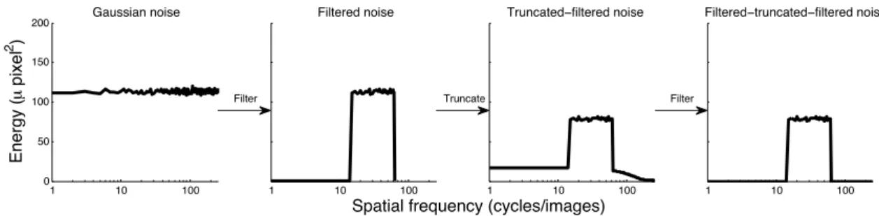
The truncation is a nonlinear operation having a frequency-dependent impact on the noise energy: it uniformly reduces the noise energy of frequencies within the pass-band and introduces energy at frequencies that were filtered out (second to third graph in Figure 7). A simple and efficient way of quantifying the energy reduction at the frequencies within the pass-band is to compare the overall energy of truncated-filtered noise with filtered noise after removing the energy introduced by the truncation operation at the filtered frequencies. This can be obtained by re-filtering the truncated-filtered noise with the same ideal filter M (third to fourth graph in Figure 7) resulting in filtered-truncated-filtered noise (NFTFG):

. (5)

Given the same expected energy distribution across frequencies for NFG and NFTFG besides a

scaling factor (second and fourth graphs in Figure 7), the expected energy ratio at the frequencies within the pass-band between these two noises (eFG and eFTFG, respectively) are

proportional to their variance ratio:

!!"!# !!" = !"#$"%&' !!"!# !"#$"%&' !!" . (6) 1 10 100 0 50 100 150 200

Spatial frequency (cycles/images)

Energy ( µ pixel 2 ) Gaussian noise 1 10 100 Filtered noise 1 10 100 Truncated−filtered noise 1 10 100 Filtered−truncated−filtered noise

Filter Truncate Filter

Since the filtering operation has no impact on the energy at the frequencies within the pass-band, the expected energy at the frequencies within the pass-band of filtered noise (eFG,

second graph in Figure 7) is equal to the expected energy at the same frequencies of Gaussian noise (eG, first graph):

, (7)

and the expected energy at the frequencies within the pass-band of filtered-truncated-filtered noise (eFTFG, fourth graph) is equal to the expected energy at the same frequencies of the

truncated-filtered noise (eTFG, third graph):

. (8) Thus, !!"# !! = !"#$"%&' !!"!# !"#$"%&' !!" , (9)

and the energy at the frequencies within the pass-band of the truncated-filtered noise is equal to:

𝑒_!"# = 𝑒_!∙!"#$"%&' !!"!#

!"#$"%&' !!" . (10)

Given Equation 1 defining the energy of Gaussian noise (eG), the energy at the frequencies

within the pass-band of the truncated-filtered noise is equal to:

𝑒_!"# = 𝜎!_{∙ 𝑤 ∙ ℎ ∙ 𝑑 ∙}!"#$"%&' !!"!#

!"#$"%&' !!" , (11)

where σ represents the standard deviation of the Gaussian distribution. Note that since energy is proportional to the noise variance (i.e., mean-squared contrast), it is trivial to equate the energy level of truncated-filtered noise at frequencies within the pass-band with the energy level of Gaussian noise (eG=eTFG’, as was done in the experiment above) by scaling its

eFG= eG

contrast by the root-mean-squared contrast ratio between filtered noise and filtered-truncated-filtered noise:

. (12)

Matlab code implementation

To facilitate the creation of truncated-filtered noise, this section provides programing code implementing the algorithm above. This code is also available in a Matlab file in

supplementary material. The novelty of the method consists in combining two successive steps: filtering and then truncating. These two simple steps are combined in function

computeTruncatedFilteredNoise, which takes two input parameters: an ideal filtering mask to

apply in the Fourier domain (Mask) and a truncation threshold (trunc). Since the filtering mask should be the same size as the noise it filters, the size of the mask matrix (including its number of dimensions) determines the size of the noise to generate. After the filtering process, the noise is truncated based on the input parameter trunc, which represents the truncation value in standard deviation of the filtered noise (as in Figure 6). For binarized-filtered noise, trunc can be set to 0. This function outputs the truncated-binarized-filtered noise

(NoiseTFG) normalized between -1 and 1 and its energy at unfiltered frequencies (energyTFG in pixels2 _{frames). Note that energyTFG is in energy units so scaling the output noise}

NoiseTFG by a contrast gain (g) would affect its energy by the square of this gain (g2).

function [NoiseTFG, energyTFG] = computeTruncatedFilteredNoise( Mask, trunc )

% Generates turncated-fitlered noise from an ideal mask %

% INPUTS:

% Mask: ideal matrix filter (0s and 1s) to apply in the Fourier domain % trunc: truncation threshold in SD

%

% OUTPUTS:

% NoiseTFG: truncated-filtered noise matrix the same size as Mask % normalized between -1 and 1

% energyTFG: energy of truncated-filtered noise in pixels^2 frames %%%%%%%% Gaussian noise (energy=1 pixel^2 x frame)

NoiseG = randn(size(Mask));

NTFG' =

RMS N

(

)

RMS N

(

)

%%%%%%%% Filtered noise

NoiseFG = ifftn(fftn(NoiseG).*ifftshift(Mask),'symmetric');

%%%%%%%% Truncated-Filtered noise (and normalize between -1 and 1)

NoiseTFG = min(max(NoiseFG/(trunc*rms(NoiseFG(:))),-1),1);

%%%%%%%% Calculate noise energy (if necessary) if nargout > 1

%%%%%%% Filtered-Truncated-Filtered noise

NoiseFTFG = ifftn(fftn(NoiseTFG).*ifftshift(Mask),'symmetric');

energyTFG = var(NoiseFTFG(:))/var(NoiseFG(:));

end

This function has the advantage of generating truncated-filtered noise for any arbitrary ideal filter (Mask). The specific choice of the ideal filter depends on the experimental paradigm. In the experiment above, the filtering was along the spatial frequency dimension, but it is also common to filter noise along the temporal frequency and orientation dimensions. The following function (computeMask) creates an ideal mask (Mask) filtering information along all or any of these dimensions. This ideal mask of nbPixels X nbPixels X nbFrames elements keeps only the information within pass-band ranges of spatial frequency, orientation and temporal frequency that are specified by the input parameters cutSpatFreq (in cycles per

nbPixels), cutOrien (in degrees) and cutTempFreq (in cycles per nbFrames), which are

vectors containing two values representing the lower and upper filtering cutoffs.

function Mask = computeMask( nbPixels, nbFrames, cutSpatFreq, cutOrien, cutTempFreq )

% Generates ideal mask filter to apply in Fourier domain %

% INPUTS:

% nbPixels: width and height of image in pixels % nbFrames: number of noise frames to generate

% cutSpatFreq: [low, high] cutoff spatial frequencies in cycles/nbPixels ([]=no filter) % cutOrien: [low, high] cutoff orientations in degrees ([]=no filter)

% cutTempFreq: [low, high] cutoff temporal frequencies in cycles/nbFrames ([]=no filter) %

% OUTPUT:

% Mask: 3D Fourier ideal filter (0s and 1s) % size = nbPixels X nbPixels X nbFrames %%%%%%% Spatial mask

Mask = ones(nbPixels);

[X, Y] = meshgrid(-floor(nbPixels/2):ceil(nbPixels/2)-1);

% Spatial frequency mask

if nargin>=3 && ~isempty(cutSpatFreq) cyclesPerImage = sqrt(X.^2 + Y.^2);

Mask(cyclesPerImage<cutSpatFreq(1)|cyclesPerImage>cutSpatFreq(2)) = 0;

end

% Orientation frequency mask

if nargin>=4 && ~isempty(cutOrien) && cutOrien(2)<cutOrien(1)+180 ratio = Y./X;

cutRatio = tan(cutOrien*pi/180); if cutRatio(1) <= cutRatio(2)

Mask(ratio<cutRatio(1)|ratio>cutRatio(2)) = 0; else Mask(ratio<cutRatio(1)&ratio>cutRatio(2)) = 0; end end %%%%%%% Temporal mask if nbFrames>1

Mask = repmat(Mask,[1 1 nbFrames]); if nargin==5 && ~isempty(cutTempFreq)

tempFreq = abs(-floor(nbFrames/2):ceil(nbFrames/2)-1);

Mask(:,:,tempFreq<cutTempFreq(1)|tempFreq>cutTempFreq(2)) = 0; end

end

The ideal mask (Mask) generated by the function computeMask can be used as an input parameter of the function computeTruncatedFilteredNoise to generate truncated-filtered noise. The following function (truncatedFilteredNoise) combines these two functions and adds input parameters (pixelsPerSpatUnit and framesPerTempUnit) enabling to convert the units of the cutoff frequency parameters (cutSpatFreq and cutTempFreq). pixelsPerSpatUnit specifies how many noise pixels are to be displayed within a given arbitrary spatial unit (e.g., degrees of visual angle) and cutSpatFreq represents the cutoff spatial frequencies in cycles per spatial units (e.g., cycles per degree of visual angle). Equivalently, framesPerTempUnit specifies how many noise frames are to be displayed within a given arbitrary temporal unit (e.g., seconds) and cutTempFreq represents the cutoff temporal frequencies in cycles per temporal units (e.g., cycles per second). The unit conversion parameters also define the units of the noise energy given by the output parameter energyTFG (e.g., in degrees2 seconds, when

pixelsPerSpatUnit represents the number of pixels per degree of visual angle and framesPerTempUnit represents the number of frames per second). For static noise, framesPerTempUnit can be omitted or set to 1, in which case the units of the energy only

represent the two spatial dimensions (e.g., degree2).

function [NoiseTFG, energyTFG] = truncatedFilteredNoise(nbPixels, nbFrames, trunc, ...

pixelsPerSpatUnit, cutSpatFreq, cutOrien, framesPerTempUnit, cutTempFreq )

% Generates turncated-fitlered noise %

% INPUTS:

% nbPixels: width and height of image in pixels % nbFrames: total number of noise frames % trunc: truncation threshold in SD

% cutOrien: [low, high] cutoff orientations in degrees ([]=no filter)

% framesPerTempUnit: noise frames displayed per temporal unit (for units conversion)

% cutTempFreq: [low, high] cutoff temporal frequencies in cycles/temporal unit ([]=no filter) %

% OUTPUTS:

% NoiseTFG: truncated-filtered noise matrix % size = nbPixels X nbPixels X nbFrames % normalized between -1 and 1

% energyTFG: energy of truncated-filtered noise in spatial units^2 x temporal units %%%%%%% Default parameters

if nargin<6; cutOrien=[]; end if nargin<7; framesPerTempUnit=1; end if nargin<8; cutTempFreq=[]; end % convert units of cutoff parameters

cutSpatFreq = cutSpatFreq * nbPixels / pixelsPerSpatUnit; % convert in cycles/nbPixels

cutTempFreq = cutTempFreq * nbFrames / framesPerTempUnit; % convert in cycles/nbFrames

% generate ideal mask

Mask = computeMask( nbPixels, nbFrames, cutSpatFreq, cutOrien, cutTempFreq);

% generate noise

if nargout<2 % (no need to calculate noise energy)

NoiseTFG = computeTruncatedFilteredNoise( Mask, trunc );

else

[NoiseTFG, energyTFG] = computeTruncatedFilteredNoise( Mask, trunc );

% convert units of noise energy from pixel^2 x frames to dva^2 x seconds

energyTFG = energyTFG / (pixelsPerSpatUnit^2 * framesPerTempUnit);

end

This truncatedFilteredNoise function provides a simple way of generating truncated-filtered noise. For instance, to generate 240 noise frames of 1080x1080 pixels that are to be refreshed at 120 Hz with 64 pixels per degree of visual angle, calling the following function:

[N, e] = truncatedFilteredNoise(1080, 240, 1, 64, [2 8], [], 120, []);

would created noise (N) filtered only along the spatial frequency dimension (2 to 8 cycles per degree of visual angle), truncated at 1 sd, normalized between -1 and 1, and of energy e degrees2 seconds.