Control applications using neural networks

CONTROL APPLICATIONS USING NEURAL NETWORKS

by

Barton Earl Showalter

S. B., Massachusetts Institute of Technology (1987)

SUBMITTED TO THE DEPARTMENT OF AERONAUTICS AND ASTRONAUTICS IN PARTIAL FULFILLMENT OF THE REQUIREMENTS FOR THE

DEGREE OF MASTER OF SCIENCE

at the

MASSACHUSETTS INSTITUTE OF TECHNOLOGY September, 1988

Signature of Author

'-I~~~~~~- _/vL,? &- ,"Department of Aeronautics and Astronautics . Approved by

N\J

Professor Wallace E. VanderVelde

Thesis Supervisor

Accepted by

,..,. --- -Professor Harold Y. Wachman

/-z'J

i_.k

..

'li.k --'uiental

_

Graduate

Committee

w~~ - I S

CONTROL APPLICATIONS USING NEURAL NETWORKS

by

Barton Earl Showalter

This research applies artificial neural networks to the field of control resulting in an augmented approach to control system design. A feedforward network, or perceptron, contains a connected mesh of non-linear, thresholding neurons that accept external inputs and compute an output based on their interconnection weights. This network operates as a variable-gain compensator in a control loop receiving the system error and outputting a control action to the inverted pendulum on a cart. A teaching algorithm adjusts the neuron interconnection weights as the controller is "exercised" through a number of position commands to the cart. The experimental results illustrate the non-linear computational advantages of the neurons and demonstrate the ability of the network controller to adapt quickly to poorly modelled or time-varying dynamics.

This report was prepared at The Charles Stark Draper Laboratory, Inc. under Internal Programs 18952 and 18867. Publication of this report does not constitute approval by the Draper Laboratory of the findings or conclusions contained herein. It is published for the exchange and stimulation of ideas. I hereby assign my copyright of this thesis to The Charles Stark Draper Laboratory, Inc., Cambridge, Massachusetts.

Permission is hereby granted by The Charles Stark Draper Laboratory, Inc. to the Massachusetts Institute of Technology to reproduce any or all of this thesis.

TABLE OF CONTENTS

1 INTRODUCTION 1

1.1 The History of Neural Networks ... 1

1.2 Advantages of Neural Networks ... .. .... 33... 1.3 Control Applications ... 3 2 PERCEPTRONS 5 2.1 Neurons ... 5... 2.1.1 Summation Function ... 6...6 2.1.2 Output Function ... ... ..66... 2.2 Perceptron Substructure ... 8

2.3 The Perceptron as a Controller . . ... 9

2.4 Network Propagation ... ... ... ... 11

2.4.1 Complete

Propagation

...

...

..

.... 12

2.4.2 One-Step Propagation . ... 12

2.5 Teaching ... 12

3 NETWORK TEACHING STRATEGIES 15 3.1 The Neural Network as a Controller ... 15

3.2 Teaching Neural Networks Using Error Propagation .. ... 16

3.2.1 The Lesson ... 17

3.2.2 Learning Rate and Momentum ... 17

3.2.3 Periodic Updating ...

...

... 17

3.2.4 Weight Initialization ... 17

3.3 Backpropagation ... 18

3.3.1 Teaching Controllers Using Backpropagation ... 18

3.3.2 Applying Backpropagation ... 19

3.4.2 Applying Forpropagation ... 21

4 THE PLANT 23 4.1 Problem Definition ... 23

4.2 Equations of Motion ... 24

5 THE REFERENCE 27 5.1 Need for the Reference ... 27

5.2 Background on Model Reference .... ... 28

5.2.1 Initial Information ... 28

5.2.2 System Reset ... 28

5.2.3 State Variables to Track ... 29

Tracking Only Cart Position and Velocity ... ... 29

Tracking All State Variables ... 30

5.2.4 Weight Update Interval . ... 30

5.2.5 Weight Update Test ... 30

5.3 Design of the Reference ... 31

6 THE NETWORK 33 6.1 The Network Control Loop ... 33

6.1.1 Variable Definitions ... 33

6.1.2 The Neural Network ... 34

6.1.3 The Plant ... 34

6.1.4 The Gain Matrices ... 35

6.2 Operation of the Network Control Loop ... 35

6.3 Controller Architectures ... ... 6...

6.3.1 The Full-State Pole Position Controller ... 37

Classical Control Technique ... 37

Analogous Network Controller .. 39

6.3.2 The Full-State Cart Position Controller ... 39

Classical Control Technique .40 Analogous Network Controller ... 42

7 THE ADAPTER 44

7.1 The Forpropagation Control Loop .. ... 44

7.2 Operation of the Adapter ... 45

7.3 Forpropagation Algorithm Derivation . ... 46

7.3.1 Gradient Descent ... 47

7.3.2 The Neuron Error ... 48

The Dynamic Sign ... 49

The Propagation Term ... 50

Final Expression for the Neuron Error ... 52

7.3.3 Weight Change Equation...52

8 IMPLEMENTATION 5 4 8.1 Neural-Network-Controller... ... ... 54

8.2

Pole-Exec

...

...

56

9.2 The Neural Network Controller ... 63

9.3 Summary of the Results ... 74

10 RECOMMENDATIONS AND CONCLUSIONS 78 10.1 Conclusions ... 8... 78

10.2 Recommendations for Further Work ... 79

10.2.1 Partial-State Feedback Controllers ... 80

APPENDIX 82 A. 1 Pole-exec.lisp ... 82

A.2 Forprop.lisp ... ... 91

A.3 Pole-dynamics.lisp

...

...

... 103

ACKNOWLEDGEMENTS

I owe a special thanks to Professor Wally VanderVelde, my thesis supervisor, for his technical guidance and patience. I hope he has learned something about neural networks through our friendly association.

Thanks also to my friends at C. S. Draper Laboratory, especially the basketball crew, to whom I apologize again for not playing in the big game. Many thanks to Bill Goldenthal, my technical supervisor, who approached me with an exciting thesis topic and allowed me to pursue some original ideas. I am also indebted to Jim Cervantes, the Lisp guru, for hours of free-lance hacking and software consulting that somehow brought the Neural Network Controller to fruition. Another rising star on the Symbolics, Doug Eberman, also provided me with a nice graphing package and overall software support.

As for general sounding block and MacYahtzee companion, that distinction must go to my officemate and Texas-Ex, Walter Baker. The "can I erase this?" board, Speed Reversi, and afternoon outings with Gambi will be greatly missed.

Thanks to Carol, Ifeanyi and the kids for being my family in Boston. Finally, thanks to Mom, Dad, and the sibs for all their long-distance support during my five year vacation at MIT.

LIST OF SYMBOLS

E error between actual and commanded plant state

f(netj) neuron output function at the value of netj

f '(netj) slope of the neuron output function at the value of net

F control force on cart (N)

g gravity (9.8 m/sec2)

G 1 gain matrix for network inputs

G2 gain matrix for network outputs

K1, K2 gains on the classical controller Xloop

K3, K4 gains on the classical controller 0 loop

L pole length (m)

L' effective pole length (m)

M cart mass (kg)

m pole mass (kg)

Mp percent overshoot

net vector containing all neuron internal states

netj sum of the weighted inputs or internal state of neuron j o vector containing all neuron external states

oj ' output or external state of neuronj

Pik propagation term from neuron i to output neuron k

Pkk propagation term for output neuron k

R residual between actual plant state and model reference state

Rh residual of input neuron h

tj target output of neuron j

u network input vector

U plant input vector containing control commands

UM model reference vector containing target plant control commands

wij connection weight from neuron i to neuron j

Awij(P+ 1) current connection weight change

Awij(p) previous connection weight change

X cart position (m)

Xc commanded cart position

X cart velocity (m/sec)

Xc commanded cart velocity

X cart acceleration (m/sec2₎

y network output vector

Y plant output vector containing state variables

YD desired state of the plant

YM model reference vector containing target plant state

Si error of neuron j

(h)

ji error of neuron j for the residual input h

E£ scalar adaptive error

co damping coefficient of classical controller 8 loop damping coefficient of classical controller Xloop

r/ learning coefficient

0 pole position (rad)

0c commanded pole position

0 pole velocity (rad/sec)

9 pole acceleration (rad/sec2)

A constant determining steepness of the sigmoid function

14 momentum coefficient

Pc coefficient of friction between cart wheels and track . YP coefficient of friction between pole and pivot

7hk dynamic sign for plant state Yh due to control command Uh

am0 natural frequency of classical controller 0 loop

1 INTRODUCTION

The emerging technology of neural networks offers intriguing computational advantages to the field of control system design. A collection of interconnected, non-linear neurons provides a parallel processing structure that can build an input/output mapping of arbitrary form. Furthermore, simple methodologies can adjust the neuron interconnection weights to teach the network new configurations. These properties, among others, motivate this research to use a neural network as an adaptive compensator in a control loop. An informed approach to the problem requires a good background knowledge of the history of neural networks briefly discussed in Section 1.1. Section 1.2 defines the desirable characteristics of neural networks relating to control system design. The specific expectations of this research appear in Section 1.3 with particular emphasis on the problem conception.

1.1 THE HISTORY OF NEURAL NETWORKS

For many years a debate between symbolism and connectionism has raged in the field of artificial intelligence. Symbolism uses a series of symbolically coded messages in a computer program to solve problems analytically or heuristically. Connectionism relies on communication by excitatory and inhibitory signals passed between simple neuron-like processing nodes known collectively as a neural network. These two fields have seen research interest in them wax and wane over the past forty years. Today both fields remain strong foundations of artificial intelligence, but a resurgence in connectionism offers many new possible applications, especially in the fields of signal processing and automatic control.

Calculus of the Ideas Immanent in Nervous Activity written by McCulloch and Pitts in

1943. Their "neuro-logical networks" with linear threshold elements attempted to exploit the computational nature and structure of biological nerve cells. In 1947, the same authors wrote a second paper, How We Know Universals, describing the first practical application of a "neural network" to recognize particular spatial patterns invariant of geometrical transformations. With these two revolutionary papers, the field of neural networks was born.

Donald Hebb's book, The Organization of Behavior, laid the foundations of learning and internal representation in networks. To this day, many learning algorithms for simple feedforward networks find their basis in Hebb's work. Minsky in 1951 built the first "mind-like" machine that used a reinforcement-based learning rule to teach a collection of forty electronic units. However, by the end of the 1950's, the advent of the serial computer shifted research emphasis in artificial intelligence from neural net-works and

learning towards effective heuristic-based programs.

With the publication of Principles of Neurodynamics by Rosenblatt in 1962, interest in neural networks again swelled. The author proved important convergence properties of simple feedforward networks with non-linear neurons. These perceptrons could solve many interesting problems using the simple methodology that punishes the effects of individual neurons which fail to contribute to a desirable output. This learning algorithm was not foolproof as it failed mysteriously on seemingly simple exercises. Later, Minsky and Papert in their book, Perceptrons, addressed this problem concluding that the limitations of such an architecture to learn is inherent in its ability to represent.

The pessimism of Perceptrons again took the field of connectionism into an ebb of activity for most of the 1970's, but the 1980's saw yet another revival in learning machines. Hopfield published a number of important papers on his completely interconnected symmetric network which associated inputs to outputs. Recently, the two

Distributed Processing proposed a new algorithm to teach perceptrons. This new rule,

termed "backpropagation", uses input/output pairs to teach a perceptron with hidden neurons. This was a significant development since a perceptron with hidden layers sandwiched between the input and output layer is capable of more complex mappings.

1.2 ADVANTAGES OF NEURAL NETWORKS

There are a number of reasons for interest in neural networks and their application to controller design. Of great importance is the way in which a network stores empirical knowledge in the neuron interconnection weights. Information is smeared across a number of units that collectively arrive at an answer. If one particular neuron fails, the effect on the stored memory is minimal and if subsequent neurons fail, the system degrades gracefully. This is a property usually not found in other adaptive approaches. Furthermore, the perceptron constructs memory through association, giving it the ability to operate effectively in a region it has yet to explore.

Neural networks are also capable of learning good behavior in new or changing environments. With the work of Rumelhart and McClelland, a perceptron of sufficient hidden layers can be taught any conceivable transfer from input to output. The application of the teaching rules is very simple and permits greater flexibility than other current adaptive routines.

Finally, the actual development of network controllers in hardware offers a tremendous speed advantage due to the parallel processing of the nodes. Hopfield investigated implementing his network on a microchip and found staggering improvements in processing time.

1.3 CONTROL APPLICATIONS

adapting quickly to poorly modelled environments using neural network technology. In the past, researchers have approached this problem in a number of ways, each with its own set of limitations. One method, called gain scheduling, builds a string of controllers designed to operate about specific linearized conditions. As the plant moves from one envelope into another the algorithm switches controllers. This brute force method requires not only good knowledge of all the possible operating regions, but also increased computer memory. Since it is constrained to a fixed table of controllers, the methodology does not allow "on the fly" adjustments. Other approaches involve current adaptive techniques which have failed to perform adequately in many situations, often "blowing up" after a long period of good performance.

This paper offers a new approach that uses the neural network as a variable-gain

compensator in the control loop. The network receives the system error and outputs the

appropriate control commands to the plant. Initially, the plant may perform poorly, but after "exercising" the network controller the weights adjust to achieve good performance. If the plant's dynamics change over time, the network senses a degradation in performance and makes the necessary weight changes. Assuming a reasonable range of operating conditions, the network continuously reviews the plant performance and adjusts the weights, resulting in an effective controller for all operating regimes.

2 PERCEPTRONS

This chapter provides background information concerning the internal mechanics of the perceptron. A neural network is a mesh of neurons that exchange signals across directed, weighted connections. A perceptron is a special network of neurons arranged in layers. Each layer only receives inputs from downstream layers and can only output to upstream layers. Section 2.1 introduces the neuron and its related processing functions. The effect of hidden layers on generating an input/output mapping are presented in Section 2.2. Section 2.3 discusses the perceptron as a controller. Section 2.4 introduces network propagation algorithms using recursive methods. Finally a brief overview of teaching a neural network is offered in Section 2.5. The material focuses mainly on the perceptron and its properties with some general comments on neural networks.

2.1 NEURONS

A neuron is an independent processing unit with an arbitrary number of inputs and one output. A signal path between neurons carries a connection weight or strength. An input to a neuron is the product of the activation along an input line and the associated weight. Each neuron performs two functions:

1) combine the weighted inputs 2) apply the output function

These two functions transform the input or internal state of the neuron to an output or external state. The aggregate effect of the functions is the input/output characteristic of the neuron which can be linear or non-linear. Linear neurons offer simplified mathematics, but

lack the important thresholding capabilities of their non-linear counterparts. Internal w ne t

wijoi

f(nej)

Figure 2.1 -Model of a Neuron

2.1.1 Summation Function

The internal state of the neuron is equal to the sum of the weighted inputs.

netj=

iji

Each incoming line contributes the product of the signal strength and connection weight to the neuron internal state.

2.1.2 Output Function

The output function alters the internal state of the neuron by applying a thresholding function.

oj = f(netj)

There are a number of candidate functions which limit the neuron output.

Hard Limiter

Figure 2.2 - Output Functions Ranging from 0 to 1

The hard limiter allows the output to assume only two values with a discontinuity at zero. The threshold contains a linear region, but the transition from linear to the limit values is again discontinuous. The sigmoid function is both nondecreasing and differentiable - a property Rumelhart and McClelland refer to as semi-linear. For input values near zero, the sigmoid appears linear and flattens gradually for large negative and positive inputs. Each of the function's output in Figure 2.2 ranges from 0 to 1, but to achieve symmetry and full representation for positive and negative values, the output must include values between -1

and 1.

Hard Limiter Threshold Sigmoid

/1LZ

Figure 2.3 - Shifted Output Functions Ranging from -1 to 1

The output function used in this research is the sigmoid in Figure 2.3 with the following equation:

f(x, )

2

-0.5

1 -Ax

where x is the input to the sigmoid and X is a constant determining the steepness of the slope at the origin.

2.2 PERCEPTRON SUBSTRUCTURE

The perceptron substructure depends on the network interface to the outside world. This interface consists of a set of designated input neurons whose internal states are fed from an outside source and a set of output neurons whose external states are the network output. In a perceptron, a layer of distinctly input neurons is in the first column, a layer of distinctly output neurons, is in the last column, and any number of hidden layers lie in between. By convention all lines carrying network input and all lines transmitting network output carry a weight of unity. Therefore, the weights that change must connect two neurons.

.4

Figure 2.4 - The Perceptron

1

The perceptron in Figure 2.4 contains m inputs, n outputs, p neurons, and h layers. The network input vector u and the output vectory are defined as:

I

/

Il

A.

The vectors of the neuron internal state net and external state o are defined as:

net = nert net2 0 = I - I r01 02

The output vector y is a subset of the output vector for all neurons, o.

2.3 THE PERCEPTRON AS A CONTROLLER

The perceptron as a compensator in a control loop establishes a mapping between its input and output neurons. The input neurons receive the measured state variables of the plant and the output neurons transmit the control variables to the plant. A simple problem

11 I V . a. I "' 0 | . 1

with two inputs and one output can be visualized in two-dimensions as a phase plot. The range of the two input values are graphed along the x and y axis. For any state of the plant there exists a value on the graph for the output.

u = f(x,y)

Though the visualization of the decision region is difficult, this argument can be generalized to any number of m inputs and n outputs.

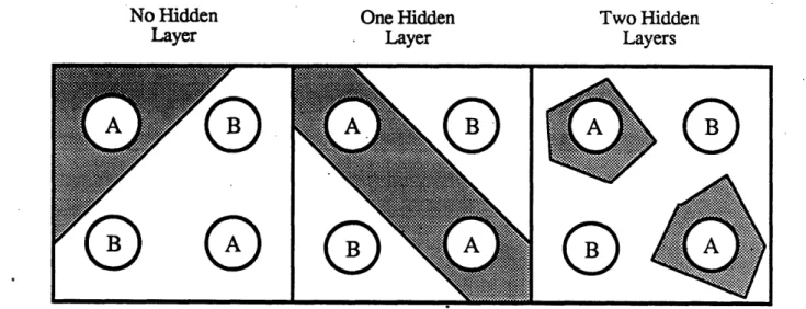
The power of a perceptron to solve a particular mapping from input to output increases with the addition of hidden layers. Furthermore, the flexibility of a perceptron depends on the complexity of the decision shape it can create in a mapping space. A simple example attempts to separate the two classes A and B in a two-dimensional mapping space. A perceptron with no hidden layer can only separate the classes by a hyperplane (or line in two dimensions). A perceptron with one hidden layer effectively separates the classes using open or closed convex regions, whereas a perceptron with two or more hidden layers can form an arbitrary boundary.

No Hidden One Hidden Two Hidden

Layer Layer Layers

Figure 2.5 - Possible Decision Regions for Various Perceptron Structures

Since the number of hidden layers defines the input/output capabilities of the network, the complexity of the desired controller dictates the network structure. If the

expected phase plane requires only linear separation of control regions, no hidden layers are necessary. As the control problem gets more non-linear, hidden layers can be added to allow for more convoluted control decision regions. However, since additional layers allow for many possible decision regions, converging on the desired set of weights becomes very difficult with more layers.

2.4 NETWORK PROPAGATION

A feedforward network propagates by updating the external states of the neurons as the internal states change. This research uses two methods to propagate the perceptron.

1) complete propagation 2) one-step propagation

Complete propagation processes each layer sequentially from left (input layer) to right (output layer). Propagation is not finished until the input signals have filtered through the network to give an associated set of outputs. The outputs are a function of the inputs and the connection weights. One-step propagation allows a signal on any line to pass through only one neuron for each time step. The outputs are now functions of the inputs, the connection weights, and the effect of past inputs held on internal lines within the network. By maintaining the impact of past inputs on the present output, the network experiences a form of memory different from resident neuron memory.

The computer simulation uses the techniques of one-step and complete propagation in an object-oriented environment. Each neuron is abstracted as a data structure and can.be told to collect its inputs, process them, and output the resulting signal. This is a local neuron update. The propagation of the perceptron depends on the order in which the local neuron updates are executed. The methodologies are identical for both linear and non-linear neurons.

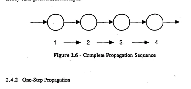
2.4.1 Complete Propagation

To achieve a complete propagation the neurons must be updated beginning with the input layer. The methodology continues updating the neurons by progressing through the network layers to the output layer. This has the effect of carrying the network input

downstream from the input layer to the output layer. The output of the last neuron reaches

steady-state given a constant input.

1

*

2

3

* 4

Figure 2.6 - Complete Propagation Sequence

2.4.2 One-Step Propagation

One-step propagation begins on the output layer and works upstream to the input layer. In this fashion, each neuron fires using old external states of neurons yet to update. This technique does not require storing of old values to achieve memory in the system.

4 - 3 4 2 4 1

Figure 2.7 - One-Step Propagation Sequence

networks are taught, some begin with a defined set of weights which never change. The basic learning rule for a perceptron proposed by Hebb increases the weights along the paths whose signals tended to produce the desired output. A weight along a path whose signal caused the output to diverge from the desired could be decreased or kept unchanged. Hebbian learning is rarely used in this simple form today, but almost all teaching algorithms are descended from this manner of adjusting the connection strength.

This research teaches the perceptron using a group of learning rules known as error

propagators. Each of these algorithms involve a number of steps.

1) Evaluate the performance of the network 2) Generate a local error at the point of evaluation 3) Propagate the local error to all contributing neurons

4) Change the weights between neurons according to their error

Error propagators employ a gradient descent in the local error with respect to weight changes.

Rumelhart and McClelland's learning rule, called backpropagation, evaluates the network performance using desired input/output pairs. The local error originates at the network output. These errors are then recursively "backward propagated" to all the contributing neurons. The connection weight between two neurons changes according to the error of both neurons. When the network operates as a compensator in a control loop, backpropagation requires knowledge of the network output or control action given an input or state of the plant. This constrains the weights to converge on a preset control law.

This research proposes a new algorithm, calledforpropagation, which generates a local error based on a comparison of the actual and target network input. This evaluation uses a desired plant state or network input instead of a desired control action to the plant. The local error originates at the inputs and is "forward propagated" to the output neurons

using a term which relates the change in input to an associated change in output. Forpropagation then proceeds like backpropagation using the neuron errors to adjust the weights. The weights then converge on values that result in a target response of the plant regardless of the necessary control action.

3 NETWORK TEACHING STRATEGIES

This chapter compares two methods for teaching neural networks which operate as compensators in a control loop. Both algorithms, classified as error propagators, use gradient descent techniques to adjust the connection weights of a perceptron with semi-linear neurons. Backpropagation is a popular method effective in many problems, but not well-suited for control applications. Since backpropagation requires input/output pairs, the

network output must be known which requires prior knowledge of the desired

compensator. This constrains the network to converge on a predetermined set of weights. As a result, a new technique termed forpropagation specifically addresses the problem of teaching a compensator. Section 3.1 discusses the architecture of a controller with a network compensator. Section 3.2 introduces issues related to the general method of error propagation teaching algorithms. Sections 3.3 and 3.4 give quick overviews of the backpropagation and forpropagation algorithms.

3.1 THE NEURAL NETWORK AS A CONTROLLER

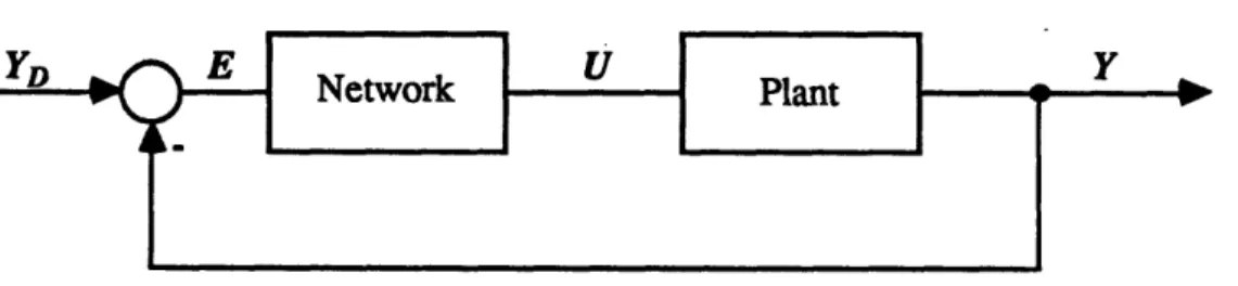
The neural network control loop (Figure 3.1) consists of a neural network in series with a plant. The network receives a desired state of the plant YD minus the actual state Y and passes the controlling inputs U to the plant.

The network acts as a compensator in the control loop. By changing the connection weights the network can produce any desirable transfer between input and output. If the network maintains memory either from resident neuron memory or through one-step propagation, then it is a dynamic compensator. A network continually taught while operating within the control loop is an adaptive compensator.

The connection weights change according to a learning rule which uses an evaluation of the network's performance as a controller. One current approach to this problem uses the backpropagation algorithm which evaluates the network output based on a desired input/output pair. Unfortunately, this requires complete knowledge of the desired control function. At best, the network will learn a target controller but cannot adjust the compensator parameters on-line.

The main theoretical contribution of this research is a second approach to teaching a network in a control loop. This new approach, named forpropagation, produces an evaluation at the network input based on the difference between the actual state variables and their commanded values. By tracking the plant state exclusively there is no need to specify an initial controller, the network converges on the weights necessary to control the plant. If the dynamics vary over time, the network senses the error and adjusts the weights accordingly.

3.2 TEACHING NEURAL NETWORKS USING ERROR PROPAGATION

The method for teaching networks using error propagation produces a gradient descent in error with respect to weight changes. At every step, the routine calculates the

aE

partial derivatives F of the total error with respect to each weight then moves a certain

aE

distance in the direction of the negative gradient vector W. Assuming no problems

3.2.1 The Lesson

Error propagation of all types adheres to a strategy of data presentation with weight changes known as the lesson structure. Sometimes the teaching session occurs off-line in a procedure calledfixed learning. After the network is taught, it is used in an application with fixed weights. Another common method involves on-line or adaptive learning. Here the weights are continuously adjusted while the network performs its function.

3.2.2 Learning Rate and Momentum

The learning coefficient T7 dictates how quickly the weights change. Ideally this is as high as possible without leading to oscillations or instability in the weight changes. An effective way to increase the learning rate while filtering out high frequency oscillations is to include a momentum coefficient I which includes the effect of the last weight change on the current change. This keeps the weights from adjusting drastically due to high-frequency noise. Some researchers set i + T7 = 1, while others let the coefficients vary freely. A typical setting would be 4u = 0.9 and = 0.1.

3.2.3 Periodic Updating

Often it is desirable to accumulate the weight change over several presentations of data and then incrementally adjust the weights. Sejnowski [27, 28] used this procedure when he presented the letters of a word sequentially and then adjusted the weights once for each word according to the summed contribution of each letter. This method allows the network to treat a sequential set of data as one.

3.2.4 Weight Initialization

Weight initialization with most teaching rules is a crucial step incorporating prior information. With error propagation the network can start as a clean slate. However, it is

necessary to initialize the weights to small random values to break the symmetry of the network and allow connections to assume different weights. Usually the weights are uniformly distributed over a small range of positive and negative numbers.

The closer the initial weights are to the desired final answer, the faster the network converges. In addition, if the starting weights are much larger than the target values, the network receives misleading information from the plant resulting in weight instability. Assuming the neurons operate in their linear region, the network weights could be initialized using the best information of the final control law. This represents a "first-cut linear guess" at the desired compensator.

3.3 BACKPROPAGATION

Backpropagation in feedforward networks employs the generalized delta rule to teach a network input/output pairs. The method adjusts the connection weights by evaluating the error of the output layer. A teaching session using backpropagation cycles through a number of input/output pairs. For each presentation, the weights change slightly to register the effect of that pair on the final network.

After a sufficient teaching period, the network possesses the ability to associate an input with a corresponding output. For example, suppose the network is taught using desired outputs that are the squares of the corresponding inputs. Also assume only the pairs of odd numbers and their squares are used to teach the network. In theory, after the teaching is complete, the network will not only output the squares of the odd number inputs, but it should also build the association to estimate the even number squares.

3.3.1 Teaching Controllers Using Backpropagation

Figure 3.2 shows the network control loop augmented by a backpropagation adapter. Since the network adjusts the weights while attempting to control the plant this is

a form of adaptive learning. The reference in the figure represents the desired compensator for the plant. The network at best can only mimic the reference. structure. If the reference compensator is poorly designed or the plant dynamics are not well known, the network controller cannot perform well. The adapter receives the residual R and applies the rules of backpropagation to the network.

Figure 3.2 - Backpropagation Control Loop

This design builds a compensator into the associative memory of the network. When the network operates as a controller, it associates certain states of the plant with approximate control actions. Unfortunately, the approach requires knowledge of a controller and assumes no plant modelling errors. In most control systems, the desired state of the plant is known but not the desired control action. This need for a desired output severely limits the capabilities of backpropagation as a teacher for a controller.

3.3.2 Applying Backpropagation

Teaching a network using backpropagation, or any other neural network teaching algorithm, requires adherence to a number of rules. Foremost, the network must be a perceptron with semi-linear neurons. Special attention must be paid to the ordering of steps

to change the weights as well as the setting of a number of teaching parameters.

Backpropagation is applied in two steps. First, the routine generates the neuron errors recursively starting at the output using the following equations for output and hidden neurons:

output neurons j = (tj -o) f'(net)

hidden neurons

6,

= f(netj) X

wjk

k

where t is the target output and oj is the actual output. Second, the weights are changed according to:

Awij ( + 1) = Tl 6i oi + p

Awij(P)

where il is the learning coefficient, # the momentum coefficient, Awi (P) is the weight change made during the previous lesson, and Awij ( + 1) is the weight change for the current lesson.

3.4 FORPROPAGATION

Forpropagation adjusts the connection weights based on an evaluation of the inputs. The weights continually adjust as the network attempts to control the plant. If the error grows too large or the plant becomes unstable, the system reinitializes and a new lesson begins. After a number of lessons, the weights converge on values that produce a desired response in the plant. Forpropagation is a natural methodology allowing the user to specify a performance for the plant. If the plant dynamics change, the network senses the error and adjusts the weights to again achieve the desired response.

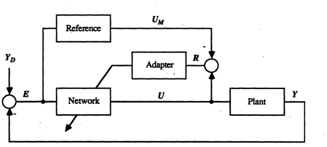
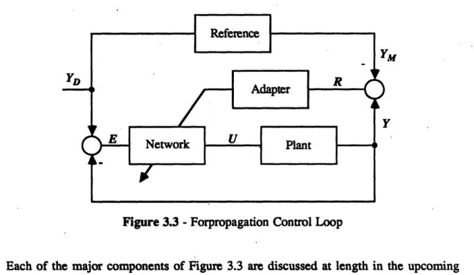
3.4.1 Teaching Controllers Using Forpropagation

adapter. The reference in the figure represents the overall desired plant response. The adapter receives a residual based on the desired and actual plant states and applies the rules of forpropagation to the network.

r

Figure 3.3 - Forpropagation Control Loop

Each of the major components of Figure 3.3 are discussed at length in the upcoming chapters.

3.4.2 Applying Forpropagation

Forpropagation, like backpropagation, requires a perceptron with semi-linear neurons. Issues related to gradient descent techniques also remain unchanged. A complete derivation of the forpropagation algorithm explaining all terms and notation appears in Chapter 7.

Forpropagation performs three operations. First, it calculates the propagation terms beginning at the output using the two equations for the output and hidden neurons:

output neurons hidden neurons

Pkk = f'(netk)

Pik = f(net,) E w ijPjk

Second, the routine generates the neuron errors 6 for both the hidden and output neurons using the residual vector R.

(h)

output neurons a8_k = -R h kP k k

(h) outputs

hidden neurons 6 = -R h hpjk

k

where rhkis defined as the dynamic sign term. A neuron error represents how

forpropagation changes the neuron's weighted sum input (i.e. - its upstream connection weights) to decrease the value of the residual. Finally, the weights are adjusted using the equation:

residuals (h)

Awij(p+

l) = oi

6 + Awij(P)

h

where 77 is the learning coefficient, p the momentum coefficient, Awij (p) is the weight change made during the previous lesson, and Awj (p + 1) is the weight change for the

4 THE PLANT

The dynamic problem chosen for the neural network controller is the inverted pendulum on a cart. This chapter defines the plant and its state variables and presents the

derivation of the equations of motion.

4.1 PROBLEM DEFINITION

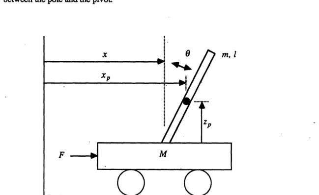
A cart rests on a straight and level track (Figure 4.1) with an inverted pole attached to its center by a pivot. The cart must remain on the track and the pole can move only in the vertical plane of the track. A control force F can be applied on either side of the cart at its center of mass. One frictional force acts between the cart wheels and the track and another between the pole and the pivot.

Full-state feedback includes the cart's position X and velocity X and the pole's angular position 0 and velocity . The two measurements Xp and Zp are used in the Lagrangian derivation of the equations of motion. The important parameters include:

g = gravity (9.8 m/sec2)

M = mass of cart m = mass of pole L = half length of pole

p = coefficient of friction of cart on track

/Up = coefficient of friction of pole on cart

4.2 EQUATIONS OF MOTION

To derive the equations of motion of the cart-pole problem using Lagrangians, first define the coordinate transformations Xp and Zp, and their first derivative:

Xp = X+Lsin8 Xp = X + LcosO 0

Zp = L cosO

Zp = - L sine

Now write the kinetic energy of the system Ek including terms for the cart's translational energy and the pole's translational and rotational-energy.

Ek = MX +m

+

+

-

-m

L

0

.2 .2 1

'2 m L2 +mLcosX

Ek = (M+m)X +mL

The potential energy of the system Ep depends only on the pole.

Ep = mgZp = mgLcosO

Now write the Lagrangian of the system.

1 .2 2.2

A =

= (M+m)X +-mL 9 +mLcosOXO-mgLcos9

The forcing terms for X and 0 are:

xx = F-c I sgn(X)

The

Xand

equations

= -balance

in

both

are

defined

as:

d aA

d.t'a

d

a

d

ax

Evaluating the above equations and rearranging gives the two equations in X describe the motion of the cart-pole.

F(t) + m L (t) sin(t) - (t) cos(t) -F(t) + m L 9 (t) sin (t) - 0t) coso(t)-) X(t)

_M+m

gsine(t) + cosO(t)

M+m

These are the two equations used in the cart-pole simulation. For a given state of the plant, and 0 that

t =

Pp 9(t)

mL

the routine first determines 8 and X and then uses a numerical integration scheme to determine the pole and cart positions and velocities. A simplified set of dynamic equations

assume:

* no friction (uc = 0 and pp = O)

*

* cart mass is much greater than pole mass (M + m = M and m = 0)

Now the equations defining the motion of the cart-pole are:

*

g

F

L L'M

F

X=-M

where L' is the effective pole length defined as:

1 L2 2

L' ML2

-ML

+ML2

4

=

ML ML 3

These simplified state equations are used in Chapter 6 to motivate an architecture for the neural network compensator.

5 THE REFERENCE

The plant and the reference controller run simultaneously and are given identical commanded positions. The reference is a simplified plant model (no friction, nominal dynamic parameters) with a linear control law that responds in a desired manner to control commands. The teaching algorithm adjusts the network weights "on the fly" according to the difference between the reference and plant states. If the deviations between the two responses becomes significant, the system is reset and a new lesson begins. After the teaching is completed, the network weights should converge on values that result in similar performance of the reference and plant.

5.1 NEED FOR THE REFERENCE

The reference is necessary due to the formulation of the forpropagation algorithm. The equations adjust the weights to achieve a gradient descent of some measure. If that measure is the system error E, the weights constantly change to decrease E. This results in unbounded weights since a newly commanded position of the cart is perceived as a discontinuous increase in E. With each teaching pass, forpropagation changes the weights to move the cart faster and faster to the commanded value. Eventually the gains of the network compensator become too large and the system reaches instability.

As an alternative approach, forpropagation uses the residual R which is the difference between the actual plant state and the desired reference state. The reference and the plant receive identical commanded positions and the reference "shows" the plant the appropriate response. Here forpropagation is well-suited to null the residual by adjusting the connection weights. If the cart is moving too fast with respect to the reference, the weights change to slow the cart down; and, if the cart lags the reference, the weights

change to speed up the response. The reference always provides the identical response characteristics for the plant to follow. If significant changes are made to the plant dynamics, the weights will again adjust to mimic the reference.

5.2 BACKGROUND ON MODEL REFERENCE

This section discusses a number of issues related to teaching with a reference. Most of the observations result from experimental work with the neural network controller

simulation.

5.2.1 Initial Information

Ideally, the initial values of the network weights are as close as possible to the final weights after convergence. In this situation, the controller slightly adjusts its internal representation to satisfy the performance requirements. However, if the initial network weights are significantly different from the target, the controller must go through an intensive and carefully structured learning session.

5.2.2 System Reset

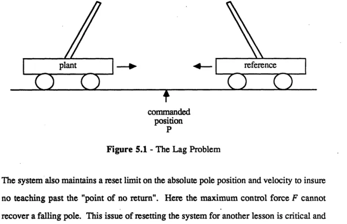
System reset is a necessary action when teaching the network in a "carefully structured learning session." As the deviations between the plant and reference increases, the chance for spurious weight change and instability also increases. Consider the simple -example when the cart-pole begins at X = 0 and is commanded to a positive position P. Assume the plant lags behind and the reference reaches P first. The reference then overshoots the commanded position and begins moving back to P with a negative X and a negative 9c. Meanwhile the plant has yet to reach P and continues with a positive X and a positive Oc. At that instant the network controller receives ill-advised information on

the desired pole position and desired cart velocity. In this situation the system should be reset.

Figure 5.1 - The Lag Problem

The system also maintains a reset limit on the absolute pole position and velocity to insure no teaching past the "point of no return". Here the maximum control force F cannot recover a falling pole. This issue of resetting the system for another lesson is critical and should be addressed with much care.

5.2.3 State Variables to Track

Tracking a state variable means comparing its value with the reference over time and generating an error used in adjusting the weights. In the cart-pole problem there are four possible state variables to track: pole position, pole velocity, cart position, and cart velocity.

Tracking Only Cart Position and Velocity

The final objective is to control the cart position so it seems logical to choose to track only the cart position and its velocity. The only requirement on the pole is that it

remains erect regardless of the time history of its position and velocity. Furthermore, with a change in cart mass or pole length, the network controller will undoubtedly require a different response in the pole to achieve the same response in cart position. This may present a problem when the network controller commands an unrealistic and irrecoverable pole position. However, the thresholding effects of the neurons do limit this action.

Tracking All State Variables

This approach is not recommended unless problems arise with keeping the pole upright. Perhaps an acceptable approach would be to leniently track the pole position and velocity to insure balancing.

5.2.4 Weight Update Interval

The weight update interval is a crucial setting in the learning algorithm. One approach updates the weights much faster than the system's highest natural frequency. This offers quick learning and recovery, but is very sensitive to higher order disturbances and noise which often lead to instability. Another approach allows the network controller to perform for a long interval of time without changing the weights. This "mimic and adjust" procedure produces a more stable system impervious to higher order effects, but relies on many lessons to teach the desired weights.

5.2.5 Weight Update Test

The simulation uses two modes of update. The mandatory or forced update always adjusts the weights at the scheduled time regardless of the performance of the network controller. This approach continuously adjusts the weights even when the plant closely follows the reference. The second method, the optional update, changes the weights only if the adapter error is above a certain threshold.

5.3 DESIGN OF THE REFERENCE

The reference controller design assumes nominal dynamic parameters - a cart mass

M of 1 kilogram and a pole length L of 1 meter. The controller commands F in the range of

±10 Newtons and limits 0c to ±15 degrees. The controller was designed using pole

placement to achieve the quickest possible response in X with a of approximately 0.7.

F = 69.3 0+ 13.2 + 4.9X+2.0(X- X )

The reference response, used by the forpropagation algorithm, first reaches an Xc of 5 m in 5.44 sec, overshoots by 4.4%, and settles to within 2% in 9.56 sec.

2 E

r

r

r

Graph 5.1 - The Reference Response

The task of this controller is to produce a reference response used in the forpropagation algorithm. The controller operates on an unchanged plant model of M = 1 kg and L = 1 m, producing the identical reference response for all of the experiments. As the plant dynamic parameters change, the network controller attempts to mimic this response from the reference. Plant perturbations in pole length or cart mass that take place

in the control loop are not reflected in the reference model, thus the reference response

6 THE NETWORK

This chapter introduces the operation of the neural network as a fixed-gain compensator for the plant in a feedback loop. The network topology is specific to the control problem. In this research, the number of input neurons and output neurons match the number of state variables and control variables, respectively. Furthermore, with the cart-pole problem, the network infrastructure resembles the inner and outer loop organization of the classical compensator.

6.1 THE NETWORK CONTROL LOOP

Figure 6.1 shows the detailed version of the network control loop introduced in the Chapter 3. The positive gain matrices G1 and G2 appear along with the localized variable naming convention.

Figure 6.1 - The Network Control Loop

6.1.1 Variable Definitions

Network states are shown as lower case letters, consistent with neural network theory development in Chapter 2. Plant states are shown as upper case letters. Define the plant input control vector U, the plant output state vector Y, and the plant desired state vector YD as:

I FTT a

I1

Uj

ti1

The network receives the system error E equal to the desired state YD minus the actual state Y and passes the controlling inputs U to the plant. The output y of the network is a function of the input u, the connection weights, and sometimes the old output states.

6.1.2 The Neural Network

The network box contains the network structure, interconnection weights, and propagation function for the perceptron. Complete propagation allows the network to settle to a steady state for each time step. The network output is a function of only the current inputs and the weights. One-step propagation passes a signal one layer forward for each time step. The output for this type of propagation is a function of the current input, the network weights, and the effects of previous input values held on signal lines within the network. This propagation incorporates memory and is used later in a design of a partial-state feedback controller. Techniques for complete or one-step propagation of linear or non-linear perceptrons appear in Chapter 2.

6.1.3 The Plant

The plant contains the control problem dynamics. It receives a control action and outputs its state variables. A full-state feedback controller uses all independent state

a Y . I

I

variables to control the plant whereas a partial-state feedback controller uses only a subset. The experimental work of this paper uses an inverted pole on a cart as the plant (see Chapter 4).

6.1.4 The Gain Matrices

The gain matrices G1 and G2 contain positive, non-zero entries along the diagonal. They are used to appropriately scale the variables of the plant and network. The gains in G_{1are chosen to keep the network input bounded by the sigmoid function. A gain on a} state variable causes the sigmoid to saturate at a particular value for that variable. This saturation point depends on the desired operation envelope of the plant. The experiments of Chapter 9 used the following four gains in G1for the state variables of the cart-pole.

The gains in G2 determine the relationship between the network outputs and the controlling inputs to the plant. For the cart-pole problem the single network output is multiplied by a factor of 10 to produce a control force range of ± 10 Newtons.

6.2 OPERATION OF THE NETWORK CONTROL LOOP

At each time step, the simulation integrates the equations of motion of the plant and updates the control action by propagating the network. At a less frequent rate, the program adjusts the network interconnection weights based on the performance of the controller. Nominally, the equations of motion and control action are updated at 25 Hz while the weights are adjusted at 5 Hz. After 5 time steps of normal fixed-gain operation, the

Gains in G1

0 8.0

o 4.0

X 0.3

network weights are adjusted. Discussion of the weight change algorithm appears in the Chapter 7.

There are three ordered events for one complete time step of the network control loop. First, the system determines the error vector:

E

=YD-Y

Next, it propagates the network, either complete or one-step, using the input vector:

u = G

E

The full-state controllers use complete propagation which allows the network to' settle to a steady-state output. Partial-state controllers require a memory of past input values and use one-step propagation. Finally, the system numerically integrates the plant dynamics using the new controlling input vector

U = G

y

6.3 CONTROLLER ARCHITECTURES

This section establishes the infrastructure of the network used as a full-state compensator for the cart-pole problem. Since all necessary state variables are available to control the plant, the compensator requires no memory and uses complete propagation. Steps are taken to develop controllers using classical methods which in turn motivate the design of analogous network structures. Section 6.3.1 derives a classical controller to balance the pole and proposes a network counterpart. Section 6.3.2 develops a compensator to control the cart position while balancing the pole and again presents an analogous network structure. Since the purpose of this section is to determine the general structure of the network compensator, a simple model of the cart-pole will suffice.

6.3.1 The Full-State Pole Position Controller

The initial task of the cart-pole problem is to balance the pole, or ideally, control the pole position. First, the problem is solved using classical control techniques and then an analogous design of a network is proposed.

Classical Control Technique

Using the simplified state equations of the cart-pole found in Chapter 4, the expression governing 0 including the forcing term F is:

O-

L'M =0

+

where g is the force of gravity, L' is the effective length of the pole, and M is the mass of the cart. Rearrange and differentiate to get the transfer function in terms of the Laplace operator s.

· S

0 L'M

The resulting control loop is:

A judicious choice of K3 and K4 places the two closed loop poles in any desired configuration. From the block diagram in Figure 6.2, assuming Oc is zero, F can be

rewritten as:

F

= -K

K

+ K40

Combine the above equation with the simplified state equation and factor out 0.

0

_{[s2 +}

_VMS

₍

_|

₊

_t~i~f,4)]

₌

₀

2 2

s

)O

where Co is the damping coefficient and o0 is the natural frequency. The two equations determining K3 and K4 for a given choice of 'o and ono are:

2

Con + _L'

K3 =

2 Co hO

K4 = 2 0nwoL' M

The preceding derivation of the O controller using classical techniques does not constrain the control input F. First choose a desired eo (usually .707) and then in an iterative procedure choose the desired aon and check if the resulting gains give a reasonable control

action. To realize a large cono requires a large control input F. After readjustment of cOno to fit within the control limits of the system, the final transfer function is:

2

0 Csteno + Lo

Analogous Network Controller

The equivalent neural network controller requires two gains on the angular position and velocity. The final network structure for the 0 controller is simple requiring only two input neurons and one output neuron.

6

6

F

Figure 6.3 - Network Structure of Theta Controller

Assuming O_c is zero and the neurons operate in their linear region, the corresponding control law as a function of the perceptron weights is:

F = w

9

+ W

(0-

)

6.3.2 The Full-State Cart Position Controller

The next task is to integrate the results of the 0 controller into a complete design to control the cart's position while balancing the pole. Again the method involves the classical approach leading to an equivalent network structure.

Classical Control Technique

The design of the control loop for X requires an important assumption. If the natural frequency of the loop is sufficiently larger than the natural frequency of the X loop, then there are two approximations. First, the transfer from Oc to 0 in the X loop is unity. With respect to the slow X loop, the loop maintains virtually no error. Secondly, the design of the X loop controller ignores the second order term in 0.

g" _@+L' = _°

This equation, using the first assumption, becomes: X g = g O_c

The block diagram for the X loop is now second order and can be written as:

Figure 6.4 - Simplified X Control Loop

This problem with the important assumptions is identical to. the loop design but with a simpler plant. Wise choices of K1 and K2 will place the two closed loop poles in any

desired configuration. With Xc treated as zero, the equation governing X is now a function of Oc

X

X[s2 + K

gs + KIK

g]=

0

Again compare this equation to the standard second order system to find the equations for K1 and K2 given a ax and w,n.

0)nx

K

1

=

2 x

K2

The X control law does not explicitly limit the internally commanded 0. Again, choose an aox and determine if it is attainable. A large AOnx in the X loop requires a large Oc which the controller may not be able to handle. It is important to define reasonable operating regions for the controller or include a limiter in the loop.

After choosing the two gains for the inner loop 0 controller and the two gains for the outer loop X controller, the final control law is:

F = K

0

-

KK

K

K

K4

- K

K

K

K

(X- X)

also in block diagram form:

Figure 6.5 - Full X Control Loop

and as a transfer function: A

X Xc

2 2

S + 2 nO s OnS

2Creones

S

+ OneL'

L

Analogous Network Controller

The network controller adopts the same assumptions as the previous section. The inner controller dynamics do not effect the outer X controller. As in the classical approach, the X loop commands a value for 9. This commanded 9 is held internally in the network configuration. Layering the two loops gives the final structure.

0

X

X

F

a

Figure 6.6 - Network Structure of X controller

Each neuron is associated with a state variable of the plant. The first layer of neurons receives the difference between the cart's desired and actual position and velocity. In this research, the value for Xc is always set to zero. The next layer receives an external signal

of the actual angular position and velocity of the pole. The network internally generates the

negative of the desired signals for pole position and velocity and feeds these values into the second layer of neurons. As a result, nodes 3 and 4 receive the difference between the desired and actual pole position and velocity. The control law as a function of the network weights with the neurons operating in the linear region is:

F = (w3 5w13+ W4 5W14) (X-X)

+ (w3 5w2 3+ W4 5W2 4) X + w3 5 0 + w4 5 0

Since there are six weights to determine four control gains, there is not a unique solution of weights for a particular control law.

7 THE ADAPTER

The adapter implements the forpropagation algorithm to adjust the network weights according to a measure of error. This error or residual is the difference between the measured state variables of the plant and their corresponding desired values. Section 7.1 presents the architecture of the forpropagation control loop. Section 7.2 introduces a summary of the operation of the adapter with emphasis on the three steps necessary to apply forpropagation. Finally, Section 7.3 shows that the forpropagation -weight change algorithm performs a gradient descent.

7.1 THE FORPROPAGATION CONTROL LOOP

The forpropagation control loop appears in Figure 7.1. The network input u and output y are lower case whereas the plant input U and output Y are upper case. G1 and G2, discussed in Section 6.1.4, are the gain matrices that scale the variables of the plant and network.

The model reference receives the commanded state of the plant YD and outputs the

desired plant response YM. The adapter uses R, the difference between the actual plant output Y and YM, to adjust the network weights. This residual R has the same dimensions

as the network input u.

I y, - ,.. \

/R, \

R =

Rj

D.

m- Mm/

\ m

The adaptive error e is a scalar and is defined as:

e=-R

₂

As e decreases, the actual plant response closely resembles the reference response. The weights are continually updated until the adaptive error e is below a particular threshold.

7.2 OPERATION OF THE ADAPTER

The adapter changes the individual neuron connection weights while the network operates as a compensator in the control loop. The adapter receives the residual R, calculates the adapter error e, and determines whether the weights should change. If is above a preset threshold, the weights are adjusted according to the forpropagation algorithm.

Forpropagation, derived and discussed in Section 7.3, performs a gradient descent in the adaptive error E with respect to network weight changes. A summary of the weight adjustment algorithm proceeds in three steps. Step 1 calculates the propagation terms p beginning at the output using the two equations for the output and hidden neurons.

m r ·

-2

-

hidden neurons output neurons

Step 2 generates the neuron errors a for b residual vector R.

hidden neurons

output neurons

Pik = f'(net)

X

oth the hidden and output neurons using the

(h)

- otuts

j)

= - Rh

k

(h)

k = -RhIghkPkk

where lrhk is defined as the dynamic sign term. Finally, Step 3 adjusts the weights using

the equation:

. residual (h)

Awij(p + l) = n oi

S

+ aw (p@)

h

where is the learning coefficient, u the momentum term, Aw (P) is the weight change made during the previous lesson, and Awj (p + 1) is the weight change for the current lesson.

After making the weight changes using these three steps, the newly taught network is used in the control loop. If the adjustments do not reduce e below a preset threshold, the process is repeated.

7.3 FORPROPAGATION ALGORITHM DERIVATION

The following is a detailed derivation of forpropagation. Many of the techniques of gradient descent parallel the work of Rumelhart and McClelland [26]. The specific subscript h is used in conjunction with the residual input R. Output neurons are denoted by subscript k, while subscripts i andj refer to any neuron. The weight that connects neuron i