An introduction to Total Variation for Image Analysis
Texte intégral
Figure


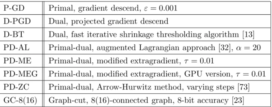
![Figure 6: Solution u for g = χ [0,1] 2](https://thumb-eu.123doks.com/thumbv2/123doknet/14503627.528316/37.892.392.603.185.401/figure-solution-u-g-χ.webp)

![Table 2: Performance evaluation of various minimization algorithms. The entries in the table refer to [iterations/time (sec)].](https://thumb-eu.123doks.com/thumbv2/123doknet/14503627.528316/62.892.232.761.189.455/table-performance-evaluation-various-minimization-algorithms-entries-iterations.webp)

Documents relatifs
It is important to note that not allowing topological changes during the descent is not an issue, since all convergence guarantees of Algorithm 1 are preserved as soon as the output
Build new convex working model φ k+1 (·, x j ) by respecting the three rules (exactness, cutting plane, aggregation) based on null step y k+1. Then increase inner loop counter k
• if the Poincar´e inequality does not hold, but a weak Poincar´e inequality holds, a weak log-Sobolev inequality also holds (see [12] Proposition 3.1 for the exact relationship
In the second part of the section, we argue that, on the Gaussian channel, the problem to be solved by neural networks is easier for MIMO lattices than for dense lattices: In low
The existence result is established using the convergence of a numerical approximation (a splitting scheme where the hyperbolic flow is treated with finite volumes and the
We then add (columns 5 and 6) the dominance and propagation rules presented in Section 2.1.4 (EQual Pro- cessing time, EQP), Section 2.2 (Dominance rules relying on Scheduled Jobs,
In [RR96], explicit bounds for the exponential rate of convergence to equilibrium in total variation distance are pro- vided for generic Markov processes in terms of a suitable
To address these problems, we propose a new model based on Bilateral Total Variation (BTV) regularization of the sharp image keeping the same regularization for the kernel.. We
