Control signal transmission through power supply cables of a 3-phase PWM motor

Control Signal Transmission through Power Supply Cables of a 3-Phase PWM Motor

by Jose A. Mendez

Submitted to the Department of Electrical Engineering and Computer Science in Partial Fulfillment of the Requirements of the Degree of

Master of Engineering in Electrical Engineering and Computer Science at the Massachusetts Institute of Technology

February 4, 2006

Copyright 2006 M.I.T. All rights reserved

The author hereby grants to M.I.T. permission to reproduce and distribute publicly paper and electronic copies of this thesis

and to grant others the right to do so.

- L_. I r 1 I

Departmen-f Electrical Engineeringp7 Computer Science February 4, 2006 Certified by Accepted bl S.. . _D•r. Chathn M. Cooke .:Thesis Supervisor-,--- . SArthur C. Smith

Chairman, Department Committee on Graduate Theses

MASSACHUSENTSOW OF TECHNOLOGY

AUG 14 2006

LIBRARIES

ARCHIVES

Control Signal Transmission through Power Supply Cables of a 3-Phase PWM Motor

by Jose A. Mendez Submitted to the

Department of Electrical engineering and Computer Science February 4, 2006

In Partial Fulfillment of the Requirements for the Degree of Master of Engineering in Electrical Engineering and Computer Science

ABSTRACT

Modem process control systems often employ accurate position or speed controlled PWM motors, which require feedback data for the drive control loop. Current methods require an independently shielded cable for feedback data transmission. This is due to

the fact that high-voltage PWM signals could easily interfere with the feedback signals, which are typically one or more orders of magnitude smaller than typical PWM signals.

We propose a "zero-wire" solution, in which the additional feedback cable used is eliminated, and the feedback data is sent simultaneously with the PWM signals in the same motor power conductors. In this study, we first analyzed the characteristics of typical feedback and PWM signals. Additionally, a standard representative motor drive

cable was carefully measured and analyzed for its wave transport characteristics. The results lead us to select an RF modulation approach in which we modulate the data signals to 900MHz. The data signals are injected and extracted from the power

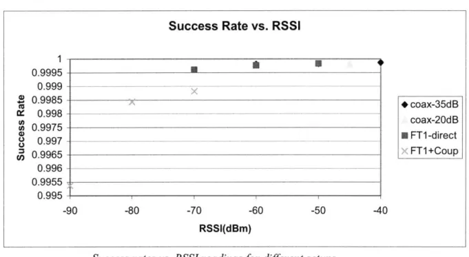
conductors using feed-through capacitors and high-pass filters. To test the performance of our approach, we build a model system in which simulated PWM signals were applied to a 30m motor power cable fitted with data couplers and 900MHz RF RS232 data modems for modulation. Tests with different cables and attenuation were performed and data error rates measured. The error rates for strong RF signals, RSSI (Received Signal Strength Indicator) values higher than -60dBm, were limited by RF modem performance to 0.01%. Error rates did not increase with or without PWM power signals when RSSI values were over -80dBm. A design for transmission of DC power for motor feedback electronics is presented, in which we choose an intermediate frequency carrier at IMHz to transmit power. The IMHz signals are injected and extracted through the same feed-through capacitors using band-pass filters. Measurements and simulation have shown that the new feedback data transport system design developed in this project is effective and feasible.

Acknowledgements:

I would like to thank my thesis advisor, Dr. Chathan M. Cooke. If not for his constant encouragement, wealth of knowledge and technical expertise, this project would not have been possible.

I would also like to extend thanks to our sponsor company, Danaher-Motion®, who provided us with all the financial support we required.

INDEX:

1. INTRODUCTION

1.1. Overview 11

1.2. The Servo-Motor System 11

1.3. Current Solution: Extra Feedback Cable 12

1.4. Zero-Wire Solution 12

1.5. Thesis Goals and Organization 13

2. THEORY AND BACKGROUND

2.1. Information Transmission in Noisy Environments

2.1.1. Introduction 14

2.1.2. Noise rejection by frequency band separation 15

2.1.2.1. Principles of operation 15

2.1.2.2. Existing examples: cell-phones, Wi-Fi, Spread Spectrum 16

2.1.3. Noise rejection by modulation 18

2.2. Current Electrical Solutions for Data over Power

2.2.1. Introduction 19

2.2.2. BPL (broadband over power lines) technologies 20

2.2.3. Home Plug (HPA) compliant 22

2.3. Motor Feeder Cable Characteristics

2.3.1. Introduction 23

2.3.2. Physical structure of motor power cables 23 2.3.3. Literature review on power cable performance 25 2.3.3.1. Frequency-domain characterization 25 2.3.3.2. Cable reflections and oscillations 26 2.4. High Frequency Conductor Losses

2.4.1. Introduction 27

2.4.2. The skin effect 28

2.4.2.1. Description of the skin effect 28

2.4.2.2. Mathematical model 30

2.4.3. Dielectric loss 32

2.4.3.1. Conduction losses 33

2.4.3.2. Dipole relaxation 33

2.5. Transmission Line Theory

2.5.1. Introduction 34

2.5.2. Ideal (lossless) transmission lines 35

2.5.2.1. Lumped-element model 36

2.5.2.2. General transmission line equations 37

2.5.2.3. Characteristic impedance 38

2.5.2.4. Propagation speed 39

2.5.3. Real (lossy) transmission lines 39

2.5.3.1. Lumped-element model 40

2.5.3.3. General transmission line equations, propagation and

attenuation constants 41

2.5.4. Finite transmission lines in TEM mode 42

2.5.4.1. Introduction to TEM 42

2.5.4.2. Reflection coefficient 44

2.5.4.3. Constant-impedance termination network 47 2.5.5. Regions of operation of a transmission line

2.5.5.1. Introduction 48

2.5.5.2. RC region 49

2.5.5.3. LC region 50

2.5.5.4. Skin-effect region 51

2.5.5.5. Dielectric loss region 51

2.5.5.6. Waveguide dispersion region 52

2.6. Serial Communication Protocols

2.6.1. Introduction 52

2.6.2. RS232

2.6.2.1. General description 53

2.6.2.2. Protocol parameters, data rate 55

2.6.3. RS485

2.6.3.1. General description 55

2.6.3.2. Protocol parameters, data rate 57

2.6.3.3. Advantages of RS485 over RS232 57 2.7. Principles of Modulation 2.7.1. Introduction 58 2.7.2. FSK modulation 59 2.7.2.1. Principle of operation 59 2.7.2.2. Mathematical model 60 2.7.2.3. Probability of error 61 2.7.2.4. Data rates 62

2.7.3. OOK, ASK, FSK ortho-normal plots 62

3. APPARATUS AND PROCEDURE

3.1. Description of Components and Devices

3.1.1. FT1 30m reference cable 65

3.1.2. Motor drive 67

3.1.3. Pulse generators 68

3.1.3.1. DataPulse 101 pulse generator 68

3.1.3.2. HP-8005B pulse generator 69

3.1.3.3. Ritec SP-801 square wave pulser 69

3.1.4. Filters 69

3.1.4.1. Feed-through capacitor box 70

3.1.4.2. Lumped external filter 72

3.1.5. 9Xtend radio modems

3.1.5.1. General description 73

3.1.5.3. Manufacturer specifications 75 3.1.5.4. Software loop-back test 75

3.1.6. Miscellaneous cables and connectors 77 3.2. Experimental Setup

3.2.1. Equipment characterization

3.2.1.1. Drive and motor setup 77

3.2.1.2. Direct FTI cable pulse response 79

3.2.1.3. Filter pulse response 80

3.2.1.4. Coupled FT cable pulse response 81 3.2.1.5. FT1 cable response at 900MHz 83 3.2.1.6. Radio modem transmission with simulated PWM signals 83

3.2.2. Measurement system 85

3.2.2.1. Tektronix TDS 3054B 4-channel oscilloscope 86 3.2.2.2. Acqumen data acquisition software 86 3.2.2.3. Noise reduction by averaging 86 4. RESULTS, ANALYSIS AND MODELING

4.1. Motor PWM Signals

4.1.1. Motor PWM signals in time domain 89 4.1.1.1. Rise time, fall time, pulse width 93 4.1.2. PWM signals in frequency domain 95

4.1.2.1. Spectral content 95

4.1.2.2. Ideal PWM spectral content 96

4.1.3. Simulated PWM signals 97

4.1.3.1. Simulated PWM in time domain 97 4.1.3.2. Simulated PWM signals in frequency domain 98 4.1.3.3. Contrast with real motor PWM signals 99

4.2. Feedback Data RS485 Signals 100

4.2.1. Motor RS485 signals in time domain 100 4.2.2. Motor RS485 signals in frequency domain 101 4.3. FT1 Cable Signal Propagation Response 102

4.3.1. Characteristic impedance 102

4.3.1.1. Single conductor active 103 4.3.1.2. Two conductors active 105 4.3.1.3. Four conductors active 107 4.3.2. Propagation delay, capacitance and inductance 110

4.3.3. Cable frequency response 112

4.3.3.1. Transfer response 112

4.3.3.2. Mathematical model 113

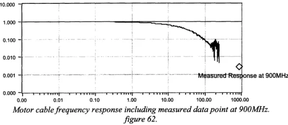
4.3.3.3. Region of operation analysis 116 4.3.4. 900MHz cable characterization 117 4.3.4.1. 900MHz cable response at different power TX levels 118 4.3.4.2. Cable mathematical transfer function at 900MHz 118

4.4. Filter Time Response 118

4.4.1.1. Transfer response 121

4.4.1.2. Ideal response 121

4.5. Model System Demonstration 122

4.5.1. Direct modem-to-modem transmission 124 4.5.2. Transmission on 50 Ohm (matched) coaxial cable 124 4.5.3. 900MHz transmission on quiet power cable 127 4.5.4. 900MHz coupled transmission on quiet cable 128 4.5.5. 900MHz coupled transmission with simulated PWM signals 130

4.5.5.1. Contrast between PWM simulated signals and real

measured motor signals 130

4.5.5.2. Error rates vs. power level 130

4.5.6. Analysis and summary of results 131

4.5.6.1. Error rates vs. RSSI 131

4.5.6.2. Error rate analysis 133

4.6. Transmission of Power for Motor Feedback Electronics 136

4.6.1. Introduction 136

4.6.2. Proposed solution and design 137

4.6.3. Simulation results 140

4.6.4. Rectification of power for feedback electronics 141 5. CONCLUSIONS

5.1. Overview of Results 144

5.2. Review of Thesis Objectives 145

5.3. Future Work 146

References 147

1. INTRODUCTION

1.1 Overview

This chapter includes a short presentation of the main issues and tradeoffs for this study which concerns data transport for servo motor control. A new improved approach is proposed and compared to present day systems. The goals for this new work and the organization of this project are also presented.

1.2. The Servo-Motor System

There are four basic components in an electrical servo-motor system. First, we need a controllable power source, the drive, which yields the variable power signals that provide power to the motor. Secondly, we have a means of transferring the power signals from the drive to the motor, i.e. a power cable. Thirdly, we require a way of measuring and controlling the motor itself, a feedback system. This feedback system, residing at the motor end measures motor status variables and relays the information back to the drive. Finally, we have, of course, the motor itself. These mechanisms are used in a myriad of applications, from food and packaging industries and electronic component

manufacturers to heavy industrial applications like precision metal cutting machines. It is this great variety of applications which produces servo motor systems with requirements which vary widely (to the extent of producing specs which differ by orders of

magnitude). The wide variety of applications and conditions make for a very interesting field of research.

1.3. Current Solution: Extra Feedback Cable

A substantial problem with servo motor systems is that interference between power and feedback signals is common. While power signals can range from 120V up to

the kV range, feedback signals are generally below the 10V range. Furthermore, power signals use PWM (pulse width modulation), which include fast transitions and thus, substantial high frequency content. For these reasons, power and feedback signals must be electrically and magnetically isolated from each other. This conflicts with the fact that

feedback and power signals must travel through similar paths, and thus physical separation is not practical. The current solution for this problem is to use two separate heavily shielded cables (or a "bundled" solution, which includes two separately shielded cables wrapped together in a larger diameter cable). This implies added costs and sizing problems. Appendix I provides a compilation of present day specifications and

requirements. This is the problem we will asses and investigate.

1.4. Zero-Wire Solution

To solve the problem of feedback transmission we propose getting rid of the extra feedback cable altogether to explore the possibility of sending the feedback data

concurrently with the same power signals in the same conductor. For the purposes of this investigation, we will focus on using all the conductors in the power cable in parallel for feedback transmission with the shielding used as a common ground. Some other options which were not studied include, for example, transmitting feedback information using two of the power cables as a balanced differential pair. This solution could help in suppressing interference and ground loop problems.

1.5. Thesis Goals and Organization

The main goals of this investigation are:

1. Characterize typical PWM and feedback signals in time and frequency domain 2. Measure the characteristics (high frequency) of a typical, affordable 3-phase

PWM motor power cable

3. Use a modulation technique (and carrier frequency) to separate the feedback signals from the PWM signals in the frequency domain

4. Design passive coupling circuits to inject and extract feedback signals without affecting PWM signal transmission

5. Create a model system to simulate real PWM signals

6. Design for transmission of DC power for motor feedback electronics 7. Test our system for reliability

8. Propose options for further investigation

Regarding the thesis organization, after this first chapter, the introduction, which serves as a quick background of the issues and the direction of this investigation, we offer a chapter on theory and background. This chapter contains theoretical

principles and background from which the system will be developed. Chapter three introduces the devices and apparatus that will be used for measurement and testing. Furthermore, this chapter will also include diagrams of the different experimental setups used for testing and data acquisition. Chapter four presents results, data, plus analysis and preliminary conclusions. Finally, chapter five includes concluding remarks and proposed directions for future work and investigation.

2. THEORY AND BACKGROUND

2.1. Information Transmission in Noisy Environments

2.1.1. Introduction

As power requirements for information transmission decrease, so does the ratio between information signal power and noise signal power. This imposes challenges for reliable, error-free information transmission. The sources of this noise can be anything from random environmental noise, such as that caused by thermal fluctuations to interference or "jamming" caused by other nearby transmitters. A simple unidirectional information transmission setup can be modeled as shown in figure 1 below:

Information transmission through a noisy channel figure 1.

The problem arises when the added noise signal power in the transmission channel is comparable to the transmitted signal power. In this case, the receiver would not be able to differentiate between information signals and induced noise signals, making the communication slow or unreliable. Of course, there are many existing solutions created to overcome this problem. Because our main purpose is to create a robust system to transmit information in the presence of motor signals, which for our purposes, can be

thought of as channel-added noise, we will briefly discuss some of the existing solutions to communication in noisy environments.

2.1.2. Noise rejection by frequency band separation

What are we specifically referring to when we talk about channel noise? Channel noise is, in its simplest terms, anything that arrives at the receiver end which was not transmitted. This includes, among other things, everything from random thermal fluctuations, signal pickup from other transmission sources, and even unaccounted nonlinearities in the transmission channel. If we look at all these noise sources in the frequency domain, they can range from white noise, with an ideally constant spectral density at all frequencies, to Gaussian noise with bell-shaped spectral density

characteristics. This immediately brings the idea of separating the noise from the signal by simply deliberately choosing transmission frequencies in which the noise levels are low.

2.1.2.1. Principles of operation

Suppose we could somehow determine the frequency fn at which a certain band-limited noise source exists, for example, in the case of our motor, this noise would just

correspond to the spectral content of the motor power signals. Then, we could choose a frequency ft such that the transmission frequency band does not interfere with the noise frequency band. The general idea of this frequency band separation is shown on figure 2:

Receiver Filter Transmitted Signal Noise Spectrum Spectrum ft fn

Noise rejection by frequency band separation figure 2.

The idea is to send a band-limited information signal at a different center frequency of that of the noise signal. Then, both signals are sent concurrently on the transmission channel. Given that we chose a center frequency for the transmission signal that is sufficiently apart from the noise frequency, the signals will not overlap in the frequency domain. Then, we can obtain our wanted signal by simply passing the received signal, noise+data through a band-pass filter centered at our transmission frequency.

This static procedure would work perfectly in a situation in which the band-limited spectral content and central frequency of the noise is predictable or well defined. Unfortunately, this is not usually the case. For example, if one is attempting to transmit

information with a mobile platform, the relative strengths, frequencies and distributions of the interfering noise signals may vary greatly. This is exactly the case for cellular phone technology. To illustrate some current solutions to this dilemma, let's look at

some existing examples.

2.1.2.2. Existing Examples: Cell-phones, Wi-Fi, Spread Spectrum

Few existing technologies have to deal with varying noise and interference as efficiently and transparently as the cellular phone. During a call, a user may move closer or further from sources of interference, for example, base stations or other users. The

quality of the transmission channel might also vary greatly, with changing line-of-sight distances and wildly changing multi-path communication. How do cell phones and other interference prone wireless technologies (such as Wi-Fi) solve this problem? The currently prevalent solution is based on a technique which was conceived in the 1940's called frequency hopping.

Frequency hopping (now usually called "spread spectrum") is a technique of communication which addresses the problems of interference and jamming. Initially considered as a way to overcome deliberate jamming of communication channels during war times, it consists on rapidly changing the center frequency of the transmitted signal. By hopping around different frequencies, the energy of the transmitted signal is spread out in the frequency domain, thus reducing the effect of sources of interference at specific frequencies.

For example, say we are attempting to transmit information at a center frequency of 100MHz. If we use narrowband transmission, any source of noise operating at a frequency of 100MHz (an FM radio station, for example), would add up directly to our transmitted signal, thus increasing our probability of error. If this same signal is instead transmitted using frequency hopping methods, although the received signal at 100MHz would be corrupted, the information received at other frequencies would not. Thus, this type of wide-band transmission attains better noise and interference rejection at the cost of utilizing a larger portion of the frequency spectrum (higher bandwidth). Variations of this spread spectrum transmission principle exist in practically any currently existing cellular phone and Wi-Fi wireless broadband technology.

This spread spectrum technology can be used more efficiently by refining the frequency-selecting algorithm. We have several options for determining how we are going to change the transmission frequency. One option is to set a certain pattern of frequencies and program this into both the transmitter and receiver. This way, we start with a certain frequency, after some determined time, move to another frequency and so on, repeating the pattern indefinitely. Another option is to select a random sequence as

our frequency transmission list. Finally, one could use a more sophisticated method, in which we first determine a relatively "quiet" piece of the spectrum and then send our precious information in that frequency. This technique is used by the HPA (home plug alliance) protocol, an Ethernet over power lines system which will be discussed with more detail on section 2.2.3.

So, we have discussed existing methods for rejecting band-limited interference noise sources, even if those are dynamic in frequency and power. The important term we need to address next is "band-limited". What about noise sources that are clearly not band limited, such as white noise? Is there a way to deal with inherently wide-band noise, optimizing our noise rejection?

2.1.3. Noise rejection by modulation

A very useful technique we can exploit to make our communication systems more robust and resistant to noise is modulation. In short, modulation is the action of taking some information signal and transforming it utilizing a given reversible algorithm such that the original signal can be recovered by applying the reverse of the algorithm. The principles of modulation and sample modulation techniques will be covered with more

detail on section 2.7. Using different principles of modulation, one can change an original data stream into a set of chosen symbols. These symbols can be represented in the transmitted signal in different ways, such as, signal amplitudes, frequency or phase. This allows us to choose modulation schemes which deliberately avoid the effects of noise by choosing symbols with sufficiently distinct representations, such that a transmitted symbol is not received as a different symbol due to noise.

2.2. Current Electrical Solutions for Data over Power 2.2.1. Introduction

The idea of utilizing existing power transmission infrastructure to transmit electrical information is not new. In the last few decades, several technologies have emerged for transmission and detection of high-frequency information carrying signals through power cables in the presence of high-voltage power signals at respectable data rates and long transmission distances. Because our purpose is to transmit data signals in the presence of high voltage power signals, it is of interest to briefly discuss some of the existing technologies to get a basic idea of how to approach our problem.

Of course, existing Ethernet over power technologies deal with power signals which are ideally sinusoidal, with a center frequency close to 60MHz. These signals, thus have very well behaved spectral content, with almost no high-frequency

components. In the case of our PWM signals, which are ideally square waves with a fundamental frequency close to 10KHz, the spectral content should spread out to higher frequencies. Thus, although the basics are similar, transmission of information in the presence of high-voltage, well defined signals, our problem is a little more complicated, with power signals that spread out in the frequency domain. Given these considerations,

let's look briefly at some of the current solutions for information transmission over power lines.

2.2.2. BPL (broadband over power lines) technologies

BPL refers to broadband over power lines, an idea which has recently developed momentum as an alternative for communication to rural areas, where power networks exist but construction of new communication networks would be too inefficient or expensive. A similar system, PLC, which stands for power line carrier has been used for many years by power utility companies for control and monitoring of remote equipment and stations. This technology uses carrier frequencies ranging from 150KHz to 490KHz in the US and from 30KHz to 150KHz in Europe for communication [12, 14]. One of the main problems that arises by using these frequency ranges is that there is significant EMI and radio signal pickup, as long power line cables, which are not manufactured for high speed or high frequency signal transmission, serve as super long antennas. This, coupled with the fact that the transmission frequencies are relatively low, result in low throughput rates which, although suitable for some monitoring and control systems, are unacceptable for high speed data transmission.

The proposed BPL protocol would use higher frequencies, between 2MHz and 80MHz. Because high power cables are not designed to carry high frequency signals efficiently, repeaters must be placed every couple of hundred meters of power line to re-amplify and relay the information down the line. Another problem which arises with this information transmission scheme is the presence of transformers and relay stations in the power network. The frequency response of high power takedown transformers has a very

low magnitude for high signal frequencies, as they are ideally designed to transmit at frequencies in the order of 60Hz. For this reason, BPL networks are proposed to work only as localized networks. In such a setup, the main information hub is located at the high voltage to medium voltage substation. Here, the information is modulated up to the

desired transmission frequency and coupled into the medium voltage line through magnetic coupling.

Magnetic coupling works by transmitting a signal from one cable to another through the mutual inductance of the cables. A simple magnetic coupler is a high

frequency transformer. Signals are transmitted through the transformer although there is no direct electrical connection between the terminals. This allows us to couple in

information-carrying high frequency signals without loading our circuitry with high voltage power signals. These signals are then sent down the medium voltage power lines.

The next barrier is the step down transformer which reduces the voltage from medium voltage to household voltage levels. There are several proposed solutions for overcoming the inefficient high frequency behavior of the transformers. The first is just to boost up the power of the information signal such that it survives the journey through the transformer. Although this is a simple enough solution, it is not very efficient. The other option is bypassing the transformer altogether. This can be achieved by

magnetically coupling in and out at the input and output side of the transformer in a similar manner in which we originally injected the signal at the substation, thus

effectively eliminating the transformer problem entirely. The last proposed solution is to use the step down transformer stations as Wi-Fi towers. A Wi-Fi transmitter is attached

at each take down transformer station and then individual users connect through the network wirelessly through the station.

Although all these ideas seem reasonable and feasible, they do not come with their own set of drawbacks, mainly EM radiation. As previously stated, power line conductors are not shielded, therefore, they will radiate eagerly when excited with high frequency signals. Wide implementation of this technology could cause serious

interference problems for short wave (HAMs) and other radios. Currently, regulations are being constructed to address this problem.

2.2.3. Home Plug (HPA) compliant

While BPL attempts transmission of Ethernet over medium voltage power lines over very long distances, there are several other technologies which exploit the power networks already available at homes and offices. HPA, which stands for HomePlug Alliance is one of the dominating protocols in this area. The technology is similar to that of BPL, except of course, that the voltage power signals that are present in user-end power drops are less than a decade below those of the medium voltage power signals

BPL is designed to operate with. One of the issues that HPA is specifically designed to deal with is drastic changes in power line network conditions. In a normal household, the properties of the power network depend heavily on many uncontrollable factors such as which appliances are running at which times. For example, devices such as electric power drills and vacuum cleaners are great sources of static which degrade the quality of the communication line. According to specifications, HPA network devices avoid these pitfalls by using a form of frequency hopping by "listening" to the power network and

determining a relatively quiet frequency to transmit information. With the use of these techniques, HPA networks are able to routinely achieve broadband Ethernet speeds of up to 14Mbps under normal working environments.

Although these technologies solve a problem which is in some ways similar to ours, our solution must, furthermore, have short delay times (less than 10us). Delay is not considered an issue for most computer networking environments, but in our case,

long delays are not acceptable, as we are designing for motor feedback control which must react quickly to any changes in the conditions.

2.3. Motor Feeder Cable Characteristics

2.3.1. Introduction

On previous sections we have addressed the problems of information transmission in noisy environments. In the following sections we will focus on the issue of the quality of our proposed conductor, the motor power feeder cable. These motor power cables are designed to transmit high voltage power signals, in which high frequency information is not essential. For this reason, motor power cables have poor high frequency

characteristics as compared to, for example, a coaxial cable. This is going to be one of the main problems to be addressed during the development of the proposed solution.

2.3.2. Physical structure of motor power cables

We will focus our research in 3-phase PWM power cables as our test system utilizes a 3-phase PWM motor. Although this might seem as a very specific case, the results are applicable to other situations, as the main issues to be encountered will be very

similar. The general structure of a 3-phase, 4-wire PWM power cable is shown in figure 3. Exernal .95cm I Conducting raid + Foil nal ator Insulated Internal Conductors

Cross-sectional view of 4-conductor motor feeder cable for a 3-phase motor Figure 3.

The structure of a general 4 conductor motor feeder cable is as follows. Four individual insulated cables are at the center of the conductor, 3 cables for the 3 phases of the motor and an additional cable for ground. These four cables are bundled together at the center of the cable and wrapped with a conducting foil and braided metal shield which is usually tied to ground. This structure is in turn wrapped in a final insulating material. The reason for the shielding in this cable might appear confusing at first. If this cable is designed for transmission of high voltage power signals, why should we care about

shielding the signals against EMI interference? After all, the signal levels in this cable will routinely exceed 100V. The truth is that this shielding is not intended to protect the power signals from EMI interference, but designed to prevent EMI radiation from the PWM signals to the outside world. Current solutions for feedback control of these motors require an additional cable for transmission of the feedback signals. In general, this feedback cable will be installed such that it lies in the same pathway as the power

cable, and a short distance from it. Thus, to prevent harmonics emanating from the power cable to couple in to our feedback signals, power cables are usually well shielded.

The final note on the physical structure of these power cables is that they can vary in length from a few meters to hundreds of meters. Some 3-phase motors are utilized in

environments in which the motor and the drive system need to be physically separated, either because of specifics of production (such as harsh operating conditions at the motor end) or because of the advantages resulting from the economies of scale of centralizing the drive system of several motors that need to be controlled simultaneously. Therefore,

some of these motor feeder cables can be substantially long, something that we must take into account for our solution.

2.3.3. Literature review on power cable performance

Although power cables are not necessarily designed for high frequency signal transmission, they are designed for transmission of relatively fast transients, as those present in PWM signals. Because this rise time is directly related to bandwidth, there is

some literature about characteristics of motor cables at frequencies higher than the usual PWM frequencies of 10KHz. All of the studies and papers found dealing with this topic characterize the power cable up to frequencies in the order of IMHz.

2.3.3.1. Frequency-domain characterization

The following figure, extracted from Moreira [10], shows the calculated characteristic impedance of an unshielded, 4 wire cable. The characteristic impedance was measured here by tying together two of the conductors and measuring the impedance between these two conductors and a third one. The fourth conductor was tied to ground.

S.

....

..

•

...

2

[lO]

lossy) and decreasing our high frequency transfer response magnitude.

Another motor feeder cable characteristic that has been studied in literature is

volthouage ringing andtest only covers frequencies up to 2MHz, we can motor end. An example sthe Moreiranning thefrom thisomeof

t•4.

6C

940

: ... Puls• a. the Motor i

02 3 4

Time Isj _{x 10}"

Motor power signal overshoot and ring at the motor end [10] Figure 5.

In this example, the PWM signal at the motor end oscillates with an initial amplitude which is double the amplitude of the transmitted signal and a frequency of about 2MHz. This high frequency oscillation can be explained as a result of signal reflections at the motor end caused by impedance mismatch between the cable and the motor. The topics of signal reflections, transmission lines and impedance mismatch will be addressed in section 2.5.

Although this short literature review gives us some insight on what the characteristics of the power cable might be at low frequencies, we need to better understand conductor frequency-dependent non idealities which might become significant factors of signal loss as the transmission frequency increases.

2.4. High Frequency Conductor Losses

2.4.1. Introduction

As we increase our frequencies of interest, many of our low frequency lumped circuit assumptions start to break down. For example, what is a lossless wire at low

700- - -. ...-- - - - ----I... ....

frequencies behaves inductively at higher frequencies. Furthermore, if we keep increasing the frequency to even higher levels, wires start introducing non-negligible losses into our system. In the following sections, we will investigate these frequency dependent non idealities of conductors to better predict and analyze how our power cable behaves at very high frequencies.

2.4.2. The skin effect

Skin effect is the term given to a phenomenon in which the series impedance of a conductor appears to increase with increasing frequency. To clarify this point, let's begin by recalling what factors constitute our calculations for series impedance. The low frequency resistance per unit length of a conductor is given by the well known equation:

1

Ro

=

Where Ac is the effective cross sectional area of the conductor and sigma is the conductivity of the material from which the conductor is constructed. The skin effect comes into play by decreasing the quantity Ac, the effective cross sectional area. Even though the physical cross sectional area of the conductor is fixed and given by the physical dimensions of such conductor, the effective cross sectional area is a function of frequency. This frequency dependent Ac gives rise to the skin effect.

2.4.2.1. Description of the skin effect

In it's simplest terms, skin effect is caused by internal magnetic fields in the conductor inducing reverse currents to rapidly changing signals at the center of the conductor and adding in-phase currents at the edges. Refer to figure 6 below.

Current induced inte magnetic field

I

the direction that intercepts the induced current

The skin effect figure 6.

Suppose we have a current in the direction shown by the large arrow in the diagram. Then, we know that:

B -ds = /Oen

,where B is the magnetic field, uO is the permeability of free space and Iencl is the current which flows through the closed surface. Therefore, the direction of the magnetic field induced by the current going into the cable as shown will be clockwise. If we construct an amperian loop as shown, positive magnetic flux is defined by the RHR as going upwards. Then, we recall that:

cE .ds = B-dA

,where E is the induced electric field around the closed curve. The expression at the right hand side simply refers to the change in magnetic flux (negative) with respect to time through the closed surface S. To comprehend how skin effect works, imagine that the input current "I" is sinusoidal and of high frequency. If the current into the conductor is increasing, the induced magnetic field is increasing and thus, there is a net negative

change in magnetic flux through the amperian loop. Because the induced electric field is the negative of the change in magnetic flux, the induced current will be in the same direction as the amperian loop, as shown. The net result is that there is an induced current through the center of the conductor that is in opposite direction of the conductor current, while there is an induced current at the surface of the conductor which is in the same direction as the conductor current. Therefore, as we increase the frequency (which increases the magnetic flux time derivative), more and more of the current will flow through the edge of the conductor, as the induced currents will effectively cancel the currents closer to the center. Figure 7 below shows the progression of effective conductive cross sectional area as we increase frequency.

K

Conductor at DC Conductor at medium Conductor at very frequencies high frequencies Reduction of effective cross sectional area due to skin effect

figure 7. 2.4.2.2. Mathematical model

Now that we have discussed the basics of what causes skin effect and how increasing frequency increases effective series impedance, we can go into some existing mathematical models to describe this behavior more precisely. There are many

choose which of these models we will explore, we need to remember why we are

investigating the skin effect. Our main purpose is to determine whether or not skin effect will be an important contribution to signal attenuation in our cable, and, if it is, how will this attenuation change with increasing frequency.

Literature agrees that, given a certain degree of approximation, the effective increase in series resistance due to the skin effect is proportional to the square root of frequency. A way to understand where this term comes from is by introducing a term commonly used when addressing skin effect: the skin depth. The skin depth, normally denoted by the Greek letter lowercase delta; 3 is the thickness of the effective

conductive area at a given frequency, and is given by [8]:

To see where the square root impedance dependence arises, recall that the effective cross sectional area is given roughly by:

Ac = i (r + )2 -ir2

which, after some manipulation, simplifies to: A, = 21r3r + ;r52

In the regions where skin effect is substantial, the skin depth, by definition must be small compared to the radius of the dead zone, thus, we can neglect the second order term, concluding that the effective series resistance is approximated by the simple equation [8]:

1 1 _

Ac 2a1r 2rf-C

which shows the monotonically increasing dependence of series resistance on the square root of frequency, as claimed by literature.

Of more importance than the absolute series resistance is the ratio of series resistance at a certain high frequency to the series resistance at DC. After all, we care about the cable having higher losses at high frequencies as compared to the losses at DC. This ratio is given by:

R(

f

)

_ 2r

_ r o f

Roc 1 2

crr2 o

-One important thing to note about this last equation is that the series resistance ratio (and thus the signal attenuation) at high frequencies is higher for cables with greater radii. This is to be expected, as there is more effective cross sectional area to be lost more quickly due to skin effect for a thicker cable. This is the reason why most high speed cables are very thin. Motor power cables have to be designed with the constraint that they must be able to efficiently carry high currents, which, unfortunately for our high speed transmission hopes, means that these cables are relatively thick for RF frequencies. Therefore, we expect skin effect to be a significant contributor to signal attenuation at higher frequencies.

2.4.3. Dielectric loss

At very high frequencies, other types of signal loss mechanisms become significant. The most notable is dielectric loss. Dielectric loss is the collective term given to any kind of signal attenuation which is caused by power dissipation in the insulating dielectric that separates the interior conductor from the exterior shield. The

two main causes of dielectric loss, dipole relaxation and conduction loss will be reviewed.

2.4.3.1. Conduction losses

Conduction losses are present at all frequencies, and refer to the fact that there are no ideal insulators in the real world. With modem materials and signal levels, though, conduction losses tend to be small. In general, conduction losses are significant when dielectrics are operating in breakdown region, where the electric field present in the dielectric is strong enough to rip electrons off the molecules of the dielectric thus producing conduction. Because we are not investigating the behavior of the cable at extremely high voltage levels, conduction losses can be neglected.

2.4.3.2. Dipole relaxation

A mechanism for dielectric loss that we might need to take into account, though, is dipole relaxation, as its effect is monotonically increasing with frequency. As shown in figure 8, a dielectric is an insulating material which is composed of molecules that polarize under the effects of an electric field. When an electric field is applied, these molecules will experience an electrostatic force forcing them to align with the field.

I I

0

Electric Field

L - I

Dielectric polarized molecules align with electric field figure 8.

I

The source for loss arises when this static figure is changed into a more dynamic one. Suppose that instead of applying a simple constant electric field we apply a rapidly changing field. Sometime during the transition between positive and negative electric field the molecules must rotate and realign, as shown in figure 9. Because this transition cannot occur instantaneously, the molecules must temporarily arrange themselves in a higher energy state before they realign with the electric field. This extra energy is then dissipated in the dielectric mostly as intermolecular friction and heat.

High Energy Transition

+ State

Dielectric

Intermediate high-energy transition state from positive to negative electric field figure 9.

At very high frequencies and signal power levels the dielectric dissipation loss can be quite significant. Microwave ovens, for example, work exploiting dielectric loss.

2.5. Transmission Line Theory

2.5.1. Introduction

A transmission line is a structure used to transfer energy from one point to

another. More specifically, in the world of electrical engineering transmission line refers to a structure which guides electromagnetic energy from one point to another. Some examples of transmission lines include coaxial cables, waveguides, and PCB buses. In the mathematical sense, as long as there is a signal return path, any signal transmission

system is a transmission line. Thus, any electrical transmission system must be a

transmission line, as KCL dictates that there shall always be a return path. Two examples of commonly used transmission line structures are shown in figure 10.

Outer Conductor

Inner

Conductor

Concentric Conductor (Coaxial) Parallel Conductor (Waveguide) transmission line transmission line

Popular transmission line structures figure 10.

Our system of interest, the motor power cable is in fact a version of the coaxial

transmission line, except with four inner conductors instead of just one. In the following sections we will develop electrical and mathematical models for these structures,

focusing on the extraction of key parameters such as characteristic impedance and propagation speed. Furthermore, we will explore high-frequency considerations and different regions of operation.

2.5.2. Ideal (lossless) transmission lines

As a first step, we will develop and analyze a model for a transmission line in which the conductors are assumed to be perfectly conducting, with zero resistivity. Although this might seem to be an oversimplification, the model we will develop predicts real behaviors very accurately for moderate to low signal speeds.

2.5.2.1. Lumped-element model

Our first step in developing a model for the transmission line is taking the

physical structure and representing it with discrete circuit components. Suppose we take a transmission line and divide it lengthwise in individual segments of length dL.

dL

Differential piece of transmission line for lumped element model figure 11.

Each of these segments can be modeled by two elements. There is some finite self inductance due to the fact that the conductor is of a finite length dL. Furthermore, there is parallel plate capacitance between the two conductors. Therefore, each segment dL can be modeled simply by an inductor in series with a shunt capacitor. Our full transmission line is just an infinite chain of such circuits:

LO LO LO LO

Lumped element model for an ideal transmission line figure 12.

2.5.2.2. General transmission line equations

Now that we have a general lumped model for our transmission line, we can attack this problem with common circuit solving techniques. Take some piece of transmission line of length dL:

LOd L i(x,t) i(x+dL,t) + + V(x,t) COd L - V(x+dL,t) dL x x+dL

Incremental piece of transmission line figure 13.

Let i(x,t) and v(x,t) be the voltages and currents in the branches at some position x down the transmission line and at some instant in time, t. LO and CO are inductance and capacitance per unit length respectively. Now, apply KVL and KCL on the circuit above to obtain:

V(x,t) dLi (x t) CdLV(x+dL,t)=

dt dt

aV(x +

dL,t)

i(x,8t) -CotdL) i(x +dL,t) = 0

Rearranging and letting dL go toequations these

i(x,t)-i(x+dL,t)= COV(x + dL,t) => -ai(x,t) Oav(x,t)

=C--~- = C ~

dL

at

aL

ot

V(x,t)-V(x+dL,t) ai(x,t) av(x,t) ai(x,t)

dL at

aL

tt

These last two equations are called the general transmission line equations, as they uniquely define the voltage and current at every point of the transmission line. 2.5.2.3. Characteristic impedance

Suppose we have an infinitely long transmission line. We know it's capacitance per unit length CO and inductance per unit length LO. What equivalent real resistance could be used to substitute the load this impedance line would present? Although finding the impedance of the transmission line might at first seem like a mathematically involved calculation (it is an infinite network), the number crunching is reduced substantially if we use a simple mathematical trick. Suppose the equivalent impedance of the infinite network is ZO. If we add an additional LO and CO, the impedance should not change, as the initial network already had an infinite chain of these structures. Furthermore, this new network is exactly the same as the original network, and thus, it must have the same impedance, ZO.

LO

z

C:

Adding an inductor capacitor pair to the transmission line does not change equivalent impedance

Using impedance analysis:

Zo = Los +- 11 Zo >

Z0 =L Z

z-B

This parameter is called the characteristic impedance of the line, and is the equivalent load that will be presented at the input end if the transmission line is very long compared to the speed of the injected signal. The characteristic impedance of an ideal transmission

line is purely real.

2.5.2.4. Propagation speed

The propagation speed of the signals down the transmission line is given by: 1

v=,-o

This equation is analogous to the equation for the speed of electromagnetic waves in free space (the speed of light), in which the permeability of free space and the permittivity of free space substitute LO and CO respectively.

We, therefore, have two independent equations relating the intrinsic characteristic values LO and CO to easily measurable quantities, the characteristic impedance ZO and the propagation speed, v. Thus, given knowledge of any two of these quantities, we can determine the remaining two.

2.5.3. Real (lossy) transmission lines

Now that we have a good idea of how an ideal transmission line works, let's try to analyze the nuances of real transmission lines, especially real transmission lines at high

frequencies. As frequency increases several factors, such as skin effect and dielectric loss (discussed in more detail in section 2.4) cause regular conductors to behave in non-ideal fashion. Because a transmission line is nothing more than two conductors with some dielectric material between them, it is plausible that the same frequency dependent non idealities that affected single wire conductors will also play a factor in transmission lines. As discussed previously, skin effect is characterized by increasing series

resistance, while dielectric loss is characterized by increasing shunt conductance. Thus, we can model these non idealities as well as other imperfections by adding some

elements to our ideal model. We can then approach this model in a manner similar to our ideal case.

2.5.3.1. Lumped-element model

Skin effect has the effect of increasing the series resistance of the conductor by decreasing it's effective cross sectional area. Thus, we can model this effect by adding a resistor in series to our model. Dielectric loss, on the other hand, has the effect of shorting out the two conductors at high frequencies. This points towards adding a shunt conductance that models this effect. The modified lumped element model is shown below in figure 15.

dL

x x+dL

Incremental piece of real transmission line with parasitic series resistance and shunt conductance

Our new lumped model is very similar to the ideal one, with the addition of a series resistance to model non-zero resistive loss in the conductor and a conductance to model signal loss due to dielectric shunting.

2.5.3.2. Characteristic impedance

An easy way to obtain the characteristic impedance of the real transmission line is to simply substitute the impedance of the resistance plus the inductance for the

inductance and the impedance of the capacitance in parallel with the conductance for the capacitance. The resulting equation is:

R±+ Ls =R + L]jw

GC

+ s G

+ Cow

The most important difference to note is that, depending on the relative magnitudes of the series resistance and conductance as compared to the impedance of the series inductance and shunt capacitance, the transmission line characteristic impedance is no longer frequency independent.

2.5.3.3. General transmission line equations, propagation and attenuation constants The general transmission line equations are derived in the same manner as for the ideal case, resulting in:

ai(x,t))

v(x,t)-i(x,t)RdL- LodL t) v(x + dL, t) = 0

at

aV(x+dL,t)

i(x,t)- CodL

at

Uv(x,t) Ri(,t)+

ai(x, t)

=

Ri(x, t)

+

L

a

ai(x,t)

=

Gv(x,t)+ Co

aL

at

By assuming that the voltage and current waveforms are sinusoidal in nature, one can obtain the propagation and attenuation constants:

y = (R + jwL) (G + jwC); y = a + jfl

The attenuation constant alpha is the real part of the propagation constant. This real part produces an evanescence in the wave transmission, thus reducing the wave energy as it travels through the line, and it is generally measured, as all the other parameters

presented so far, per unit length.

2.5.4. Finite transmission lines in TEM mode

So far we have addressed transmission lines of an infinite length. Not only is this a purely theoretical construct, but infinite transmission lines defeat the main purpose why we study transmission lines at all. In an infinite transmission line, any signal injected into one end will travel forever down the line, never to be recovered. Although we could waste power sending signals down infinite transmission lines in the name of science, it is much more interesting to be able to measure and compare signals at the input and output terminals of a real, finite, terminated transmission line. In the following sections, we will develop a model to analyze transmission and reception of signals through finite

2.5.4.1. Introduction to TEM

The lumped transmission line model in which we have based all our analysis so far implies an important assumption that we must address now. In our proposed model, there is shunt per length capacitance, but no series capacitance. In the same manner, there is series per length inductance, but no shunt inductance. This implies that, for example, that the magnitude of the electric field in the direction of the wave propagation must always be 0. If this was not the case, then we would need some equivalent series capacitance to model this field. In the same way, we cannot have any magnetic field in the direction of the wave motion. This specific mode of operation, in which the

magnitude of both the magnetic and electric field in the direction of wave propagation is always 0 is called TEM. More specifically, TEM stands for transverse electro-magnetic, mode in which the magnetic and electric fields are always orthogonal to the direction of motion. Furthermore, we can argue that the magnetic field and electric field are

orthogonal to each other as they are for electromagnetic waves. Therefore, for a transmission line in TEM mode the electric field is orthogonal to the magnetic field which is orthogonal to the direction of wave propagation.

Mal f Direction of wave propagation field

Electro-magnetic fields in a transmission line in TEM mode figure 16.

Figure 16 above shows a transmission line being excited in TEM mode. As previously stated, the magnetic and electric fields are orthogonal to the direction of propagation and to each other. Furthermore, the direction of propagation is given by the cross product of the electric and magnetic fields; ExB.

2.5.4.2. Reflection coefficient

Suppose we excite a finite transmission line in TEM mode. What happens to the signal once it arrives at the other end of the transmission line? Figure 17 shows the propagation of a voltage pulse down a finite transmission line terminated in some arbitrary impedance ZL.

lin Iref

IL

Voltage pulse traveling down afinite, terminated transmission line figure 18.

A voltage pulse, Vin is applied at the input end of the finite transmission line. The current lin that this pulse will induce is set by the characteristic impedance of the line:

V

InZo

When the voltage pulse arrives at the line termination impedance ZL, this impedance will force a new voltage/current ratio according to Ohm's law. Because current flow must be conserved, the remaining current that ZL does not sink must be reflected back to the transmission line. The ratio between the magnitude of the reflected voltage pulse to the incident voltage source is given by the reflection coefficient, denoted by uppercase gamma:

F- ZL - Z

ZL + Zo

To understand the intuitive meaning of this expression, suppose ZL=infinity, or in other words, the load end is left open circuited. In this case, the reflection coefficient is

1. What this means is that all of the energy of the transmitted pulse is reflected back from the load. If instead we short-circuit the load end; ZL=O, the reflection coefficient is -1. What this means is that the traveling wave arrives at the load end, finds the short circuit and continues traveling on the opposite conductor of the transmission line.

Because we had already defined as positive voltage the difference between the voltage at one conductor minus the voltage at the other, this kind of transmission results in just a sign reversal, as predicted by the reflection coefficient. Finally, if we set the termination impedance equal to the characteristic impedance of the transmission line, the reflection coefficient is zero. In this condition, the transmission line is said to be "matched". Because the load impedance forces the same voltage/current ratio as the transmission line, all of the energy of the pulse is transmitted to the load and dissipated there, thus, there is no wave reflection. This leads to an experimental way of determining the

characteristic impedance of an arbitrary finite transmission line. Using a pulse generator, one can send voltage pulses down a transmission line. Then, change the load impedance while observing the voltage vs. time waveforms at the load end. The characteristic impedance of the line is then just the impedance at the load that results in no reflections at the load end. This technique will be essential to developing our transmission line model of the motor power cable.

Although it is not desired for most practical purposes, the reflection coefficient does not need to be purely real. For example, suppose that the load impedance is not

purely resistive but a network which contains both passive and reactive components. Because the load impedance is frequency dependent, the reflection coefficient will also be frequency dependent. This is generally not desired because it implies that different frequencies will be transferred and reflected in different magnitudes. For waveforms that are rich in harmonics, such as square waves or triangle waves, this causes distortion, which, depending on the degree of frequency dependence of the load impedance, could prove to be unacceptable.

In our case, because we are attempting to couple our high frequency signals in and out of the cable using capacitors, we have to deal with the problem of frequency dependent reflection coefficients. We will approach the problem of our detector as a pure impedance-matching problem, without diving into the minutia of how our detector works. Therefore, suppose we are given the transmission line termination shown in figure 19 below:

zo

Transmission line with an additional capacitive termination figure 19.

The load impedance is inherently frequency dependent. This is easy to comprehend if one considers what happens for high and low frequency components. For very low frequencies, the impedance of the capacitor is very large, so the load impedance

of the capacitor is very small, so the load impedance approaches the parallel combination of ZO and R, which is always less than ZO.

2.5.4.3. Constant-impedance termination network

Now, suppose that we wanted to minimize distortion caused by this frequency dependent load. One solution is to use an inductor-resistor string to balance out the decreasing impedance of the capacitor-resistor string. The proposed circuit is shown on figure 20:

Cable

Proposedfrequency-independent load termination diagram figure 20.

For very high frequencies the inductor impedance is large, while the capacitor impedance is small, therefore, the total impedance approaches RIIRc. For very low frequencies the opposite effect happens and the total impedance approaches RIJR1. Thus, it is plausible that if we choose our component values correctly, we might be able to cancel the effect of the capacitor pole with the inductor zero to get a constant impedance network if we make Rc=R1.

To approach this situation, let's first calculate the total impedance of the network:

Zq =

RI

Rc +

II(RL + Ls)

which, after some manipulation yields:

...

...

R (RL + Ls)(1 + RCs)

Zq _{RCs(Ls +RL)+(1+RcCs)(R + R}

L + Ls)

To simplify the equation above, define three time constants:

L

r = RcC, rL = , rx = RLC

RL Then the impedance equation "simplifies" to:

RRL (1+ Ls)(1 + r,.s)

Z·q

RR,Cs(1 + rs)+(l+ cs)(R + RL + Ls)

By inspection of the above equation, it is clear that setting r, = r, makes it possible to factorize the denominator and achieve a pole-zero cancellation:

RR, (1+

zcs)

e R(rxs +1)+RL (1+ TLs)

Finally, setting rL = r, = z" results in an additional cancellation:

RRL

Z

-

L = RI Ii

R +RL

Thus, the impedance of the network is frequency independent and has a magnitude equal to the parallel combination of the capacitor/inductor resistor and the shunt resistance. Finally the value of inductance that would achieve this is given by:

L = R2C

2.5.5. Regions of operation of a transmission line 2.5.5.1. Introduction

Although the model we have developed is useful to predict the behavior of transmission lines in general, because of their distributed nature, different specific

operating conditions might lead to vastly different behaviors. For example, suppose that we could cut a transmission line down to the point that it's well modeled by a single LC network. In this case, instead of experiencing the usual ZO input impedance for a relatively long transmission line, we would see just a simple LC divider network. The factors that determine how relatively "long" or "short" a transmission line is are its physical length and the frequency of interest. The table shown below in figure 21, extracted from the book High Speed Signal Propagation: Advanced Black Magic, shows the different regions of operation for different trace lengths (this book is focused on integrated circuit design, so instead of referring to transmission lines, it refers to traces) and frequencies of interest:

- 10000 - 1000

-

_I00

-

_.1

10 10' 1o0 107 l0s 10 10'" Operating frtequency (Ilz)

Regions of operation for different trace lengths and operating frequencies [8] figure 21.

In the following sections, we will briefly discuss the different regions of operation and their characteristics. The lumped-element region, corresponding to the combination of

1000 10) -0010 P .01 .)0 !