HAL Id: inserm-00664037
https://www.hal.inserm.fr/inserm-00664037
Submitted on 30 Jan 2012HAL is a multi-disciplinary open access archive for the deposit and dissemination of sci-entific research documents, whether they are pub-lished or not. The documents may come from teaching and research institutions in France or abroad, or from public or private research centers.
L’archive ouverte pluridisciplinaire HAL, est destinée au dépôt et à la diffusion de documents scientifiques de niveau recherche, publiés ou non, émanant des établissements d’enseignement et de recherche français ou étrangers, des laboratoires publics ou privés.
Mapping of low flip angles in magnetic resonance.
Fabien Balezeau, Pierre-Antoine Eliat, Alejandro Bordelois Cayamo, Hervé
Saint-Jalmes
To cite this version:
Fabien Balezeau, Pierre-Antoine Eliat, Alejandro Bordelois Cayamo, Hervé Saint-Jalmes. Mapping of low flip angles in magnetic resonance.. Physics in Medicine and Biology, IOP Publishing, 2011, 56 (20), pp.6635-47. �10.1088/0031-9155/56/20/008�. �inserm-00664037�
Mapping of low flip angles in magnetic resonance
Fabien Balezeau
1, Pierre-Antoine Eliat
2, Alejandro Bordelois Cayamo
3and Hervé Saint-Jalmes
1,41 L.T.S.I., INSERM U642, Université Rennes 1 2 PRISM, IFR 140, Université Rennes 1
3 Centro De Biofísika Médica, Universidad de Oriente, Santiago de Cuba 4 CRLCC Eugène Marquis, Rennes
E-mail:
[email protected]
Abstract Errors in the flip angle have to be corrected in many MRI applications, especially for T1 quantification. However, existing method of B1 mapping fail to measure lower values of flip angle despite the fact that these are extensively used in dynamic acquisition and 3D imaging. In this study, the nonlinearity of the radiofrequency transmit chain, especially for very low flip angles, is investigated and a simple method is proposed to determine accurately both the gain of the RF transmitter and the B1 field map for low flip angles. The method makes use of the Spoiled Gradient Echo sequence with long TR, such as applied in the double-angle method. It uses an image acquired with a flip angle of 90° as a reference image that is robust to B1 inhomogeneity. The ratio of the image at flip angle alpha to the image at flip angle 90° enables us to calculate the actual value of alpha. The present study was carried out at 1.5T and 4.7T, showing that the linearity of the radiofrequency supply system is highly dependent on the hardware. The method proposed here allows us to measure the flip angle from 1° to 60° with a maximal uncertainty of 10% and to correct T1 maps based on the variable flip angle method.
Introduction
Knowledge of the actual flip angle and its spatial distribution is necessary in many MR applications, especially for T1 quantification (Venkatesan et al, 1998; Cheng et al, 2006; Deoni S, 2007; Treier et al, 2007; Schabel and Morrell, 2008). The problem has been well known since the early quantitative work on MRI, and many B1 mapping methods have subsequently been developed (Pelnar, 1986; Murphy-Boesch et al, 1987; Akoka et al, 1993; Insko and Bolinger, 1993; Stollberger and Wach, 1996; Cunningham et al, 2006; Dowell et al, 2007; Yarnykh, 2007; Morrell, 2008; Wang et al, 2009; Schär et al, 2010; Weber et al, 2010; Sacolick et al, 2010; Chang, 2011). Latest developments have mainly focused on in vivo imaging as well as accelerated sequences to enable 3D acquisition. The current trend is to perform rapid 3D flip angle mapping to correct 3D T1 maps calculated with the variable flip angle method (VFA). Studies on the optimization of the T1 measurement (Imran et al, 1999; Cheng et al, 2006; Deoni, 2007; Fleysher et al, 2007) have shown that low flip angles (20°) or even very low flip angles (<4°) are required when using VFA using the Spoiled Gradient (SPGR) echo sequence and short TR. However, none of the existing B1 mapping methods really lays emphasis on obtaining accuracy for low flip angle values. An analysis of existing methods (Morrell and Schabel, 2010) has shown that the performance of three of the most common methods is degraded, to different degrees, with decreasing flip angle. An additional restriction concerns all approaches based on a pair or set of proportional flip angles, such as applied in double-angle methods (Insko and Bolinger, 1993; Cunningham et al, 2006; Wang et al, 2009), the phase-sensitive method (Morrell GR, 2010) or the method of (Akoka, 1993) based on a stimulated echo: the radiofrequency supply system must be linear. If this condition is not satisfied, methods based on proportional flip angles become fundamentally flawed. Our study shows that the RF transmitters do not always provide the appropriate B1 field for a nominal flip angle, especially for the lowest flip angles. As a result, we propose a simple approach to determine both the gain of the RF transmitter and the spatial variations of the B1 field with a precision that does not decrease for low flip angles.
Materials and method
Characterization of the output RF pulse magnitude
The length, the magnitude and the shape of a radiofrequency pulse determine the flip angle of the magnetization. Generally, for a given sequence, the flip angle is proportional to the magnitude of the pulse. However, if the amplifier or other components of the RF supply system are used outside their range of linearity, this leads to significant bias in the resulting flip angle. Some effects of RF amplifier distortion on slice selection were studied by (Chan et al, 1992). To quantify the effect of this nonlinearity in commonly used pulses, we carried out direct measurements of the resulting pulse magnitude as a function of the nominal flip angle, at constant pulse length. A radiofrequency probe and oscilloscope (DSO6032A, Agilent Technologies) were used to register the waveform of the RF pulses and measure their magnitude. Measurements were performed using two MR imaging systems: a whole-body Avanto 1.5T scanner (Siemens, Erlangen, Germany) using the body coil for transmission and a Bruker Biospec 4.7T scanner (Bruker Biospin, Rheinstetten, Germany) with a 36-mm linear volume coil for transmission. At 1.5T, 1-ms hermite pulses (Blümich, 2000) were registered for nominal flip angles of 1, 2, 3, 4, 8, 16, 32, 64 and 90°. At 4.7T, 1-ms sine cardinal pulses (Blümich, 2000) were registered for nominal flip angles of 1, 2, 3, 4, 5, 6, 8, 10, 12, 15, 20, 25, 30, 40, 50, 60, 70, 80 and 90°. The probe was placed at the centre of the receiver coil and all measurements falling outside the linearity range of the RF probe were discarded.
The Low Angle Mapping method
Our method is based on the same sequence used in the double-angle method: a SPGR sequence with a long TR (ideally TR>5T1), to obtain a flip angle weighting. The general expression of the SPGR sequence (Haase, 1990) is given by equation (1).
€
S = M
01− e
−TR T1
.sin
α
1− cos
α
.e
−TR T1e
−TE T 2* (1)With sequence parameters satisfying TE<5T2* and TR>5T1, the expression of the signal can be approximated by the equation (2). For low flip angles, the signal is poorly T1 weighted, thus the TR can be reduced. For example, at 10°, TR can be equal to T1 and at 1°, TR can be equal to 0.1T1.
€
S = M
0sinα
(2)Under the conditions of equation (2), the signal variations due to B1 inhomogeneity will be negligible if the flip angle is equal or close to 90°. Indeed, the signal variations between 82° and 98° do not exceed 1% of the 90° signal. In our approach, the signal of the image acquired with a 90° flip angle is considered independent of the flip angle, and is used as a reference value of M0. In other words, the 90° image provides a map of the other sources of inhomogeneity in the signal, arising from B0, M0 and the sensitivity of the receiver coil. By dividing the image at the nominal flip angle alpha by the 90° image, we obtain the sine of the actual flip angle alpha.
€
α = arcsin
S
αM
0= arcsin
S
αS
90° (3)The theoretical range of the method includes flip angles from 0° (excluded) to 90° (excluded), with a decreasing precision for flip angles close to 90°. However, the method is most advantageous when the flip angles are in the range from 1° to 20°, to the extent that the flip angle is equivalent to the ratio Sα/S90°. Considering that Sα<<S90°, the Angle to Noise Ratio of the flip angle map is equivalent to the Signal to Noise Ratio (SNR) of the image at flip angle alpha. Consequently, the method is able to map extremely low flip angles, despite the fact that because of the use of magnitude in signal processing, a non-zero mean value of the noise will appear and may be wrongly assigned to a signal value. Practically, this problem can be avoided by using a short TR at low flip angles and increasing
the number of averages of the signal for the same total acquisition time. Thereby, even for very low flip angles, a good precision can be achieved without increasing the acquisition time.
Accuracy analysis
We used MATLAB (Mathworks,USA) to simulate the accuracy of the Low Angle Mapping (LAM) method and establish the main guidelines for using this approach. The three most important sources of errors were investigated: the actual effect of B1 inhomogeneity on the 90° reference image, the effect of the T1 weighting and the noise on the signal. Since the approximation of negligible effects of B1 on the 90° signal is a key assumption of the flip angle estimation, the effects of a bias on the 90° flip angle needs to be studied to determine the limits of the LAM. The method is symmetrical around 90°, so biases of +10° or -10° will result in the same flip angle map. We simulated actual flip angles of 70°, 75°, 80°, and 85° for the reference signal, instead of a nominal flip angle of 90°. Like the DAM, the residual T1 weighting is a source of error and cannot be totally avoided in conditions of in vivo acquisitions. For example, accurate B1 mapping in brain, while satisfying the condition TR>5T1, would need a TR of 10s. Finally, we characterized the precision of our method within its valid range by means of Monte Carlo simulations. The performances of the double-angle method and our method were simulated using an identical SNR. For both methods, we simulated 30 000 samples of the signal with an added Gaussian noise for 90 flip angle values from 1° to 90°. Then, the resulting flip angle samples and their probability density functions were calculated. The cross-comparison with other flip angle measurement methods is based on two studies (Wade and Rutt, 2007; Morrell and Schabel, 2010) analysing the efficiency of the best known methods: the Double-Angle Method (Insko and Bolinger, 1993), the phase sensitive method (Morrell, 2008) and Actual Flip-angle Imaging.
Experimental validation: B1 maps and application to T1 correction
Experimental validation was performed using the TO4 test-object (Spinsafety Ltd, Rennes, France). TO4 is a cylinder containing a CuSO4 solution, which surrounds an assembly of 12 glass tubes filled
with MnCl2 solutions having T1 values ranging from 100 ms to 1000 ms. Both at 1.5T and 4.7T, T1
reference values of the test objects were obtained using several SE measurements, with chosen values of TR optimized for each tube (Spandonis et al, 2004). On the 1.5 T scanner, a set of SPGR images was acquired for B1 mapping with TR=2000 ms, TE=2.4 ms, alpha=[1 2 3 4 5 9 32 90]°, matrix size of 128x128, FOV 230 mm x 230 mm, 12 slices, slice thickness=5 mm; bandwidth= 55 000 Hz, 4 min 16 s imaging time per flip angle. Then, a set of SPGR 3D images for T1 mapping was acquired using the parameters: TR=6 ms, TE=2.4 ms, matrix size 256x256x48, alpha= [2 4 8 16 32 64]°. A 16-channels head coil was used as a receiver. On the 4.7T scanner, a set of SPGR images was acquired from one MnCl2 tube of the TO4 assembly, with TR=800 ms, TE=2.4 ms, alpha=[3 4 5 8 9 10 12 16
17 25 30 60 90]°, bandwidth=50 000 Hz, matrix size=64x64, FOV=56 mm x 40 mm. T1 maps were drawn up with a SPGR sequence at TR=6ms, TE=2.4 ms alpha=[4 6 8 10 30 60 90]°, using the same geometry and bandwidth as the B1 maps. The 36mm volume coil was used for both transmitting and receiving. Images were processed using ImageJ (National Institute of Health, USA). Flip angles maps were calculated with LAM, and T1 maps were calculated with VFA firstly using the nominal flip angles and then the measured flip angles.
Results
RF measurement
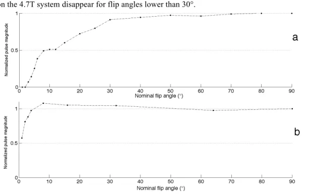
Figure 1a shows the normalized output RF pulse magnitude as a function of the nominal flip angle for the 1.5T Siemens system, while Figure 1b shows this same function for the Bruker 4.7T system. Values are normalized as a fraction of the 90° magnitude. A constant value of 1 is expected for a perfectly linear RF transmitter. The transmitter of the Siemens system is linear in the range 5° to 90°. The transmitter of the Bruker system using the 36-mm volume coil for transmission is linear only for flip angles above 30°; flip angles lower than 4° were not registered because the measured signal was too low to be in the linearity range of the RF probe used. An alteration of the pulse shape is observed
for low flip angles. Because of the limited dynamic range of the modulator, the lobes of the sinc pulses use on the 4.7T system disappear for flip angles lower than 30°.
Figure 1 Normalized magnitudes of the radiofrequency pulse for flip angles ranging from 1° to 90°. (a) Bruker Biospec 4.7T, with a 36-mm inner diameter volume transmitting coil (b) Siemens Avanto 1.5T, with body transmitting coil
Simulations of performance
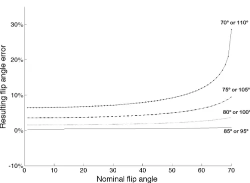
Figure 2 shows the error on the flip angle estimation caused by different magnitudes of error in the 90° flip angle. An increase in the error on the 90° flip angle has two visible effects. At first, the maximal range of flip angle that can be measured is reduced by the absolute value of the error. The second effect is a systematic overestimation of the measured flip angle. An error of 5° has a negligible effect on the accuracy of the calculated flip angle. An error of 10° results in an overestimation of 1% for flip angles ranging from 1° to 50°. An error of 20° results in an overestimation of 7% for flip angles ranging from 1° to 30°.
Figure 2 Bias on the estimated flip angle value due to inhomogeneity or systematic error
of 5°, 10°, 15° and 20° in the 90°-flip angle
Figure 3 shows the error on the flip angle estimation caused by a residual T1 weighting. The relative error does not depend on the flip angle measured. There is an overestimation of 15% of the actual flip angle value for TR=2T1 and 5% for TR=3T1, while the error is negligible for TR>5T1.
Figure 3 Error in the flip angle estimation caused by residual T1 weighting
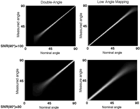
Figure 4 shows the probability density functions of the LAM and the DAM. While the precision of the double-angle method degrades for flip angles lower than 20°, the precision of our method is almost constant for flip angles ranging from 1° to 70° and degrades for flip angles higher than 70°.
Figure 4 Monte-Carlo simulations of the probability density functions of our method and the double-angle method. At top, with SNR=100 for the 90° image. At bottom, with SNR=30 for the 90° image.
Experimental B1 maps and T1 correction
The figure 5 shows flip angles measured with the Low Angle Mapping method versus nominal flip angles.
Figure 5 Flip angles measured with the low angle mapping method versus the nominal flip angles. a) on the Bruker 4.7T system and b) on the Siemens 1.5T system.
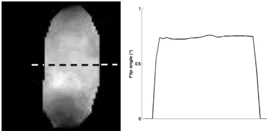
Figure 6 presents the flip angle map on the 1.5T Siemens system. The actual mean flip angle is 15% lower than the nominal flip angle, with a spatial variation of 0.2°.
Figure 7 presents corrected and uncorrected T1 maps of the TO4 test object. Reference T1 value of 380ms was obtained with optimized SE measurements for the CuSO4 solution in the body of the test object.
Figure 6 Flip angle map and corresponding cross-section in the TO4 test-object at 1.5T for a nominal flip angle of 2°
Figure 7 T1 maps of test-object using VFA (flip angles=[2,16]°, TR=6 ms) at 1.5T. (a)
Uncorrected T1 map. (b) T1 map corrected with maps of both flip angles used. (c) Cross-section following the white dashed line on the uncorrected (dotted line) and corrected (solid line) T1 maps
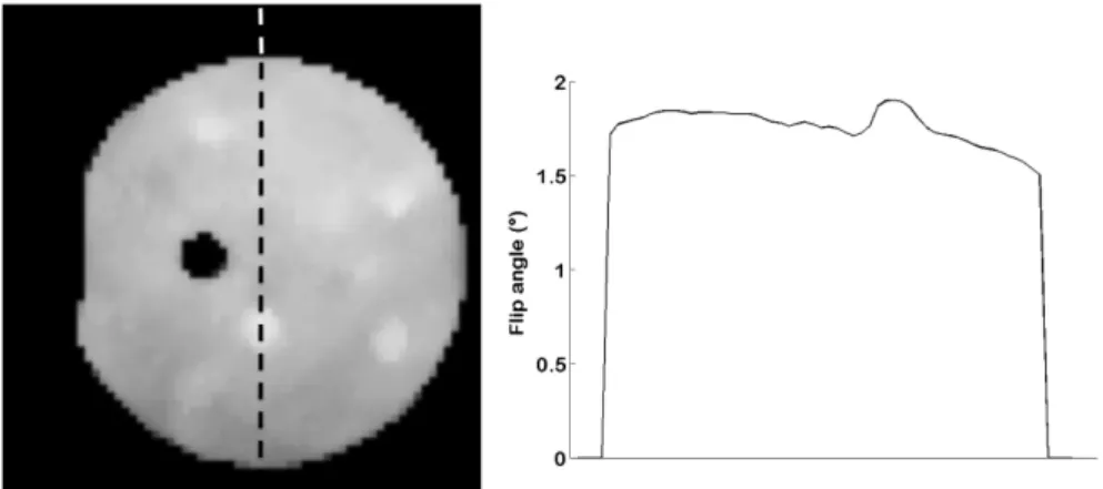
Figure 8 presents the flip-angle map at 4.7T, for a nominal flip angle of 4° with a 36-mm volume coil. The actual flip angle determined with the LAM method is 5 times lower than the nominal flip angles. For very low flip angles, the nonlinearity of the transmitter is a predominant source of error in relation to the B1 inhomogeneity.
Figure 9 presents the uncorrected and corrected T1 maps calculated with VFA at TR=6 ms and flip angles of 4° and 30°. According to the SE reference measurements, T1 should be equal to 122 ms for the MnCl2 tube. In this case, the flipangle error leads to the measurement of a negative T1 value of -25 ms without correction. With correction, we obtain a measured mean value of 130 ms.
Figure 8 Flip-angle map and corresponding cross-section in the MnCl2 tube at 4.7T for a
nominal flip angle of 4°
Figure 9 T1 maps of the tube MnCl2 tube using VFA (alpha=[4, 30]°, TR=6 ms). (a) Uncorrcted
T1 map. (b) T1 map corrected with the flip angle map. (c) Cross-sections of uncorrected (dotted line) and corrected (solid line) T1 maps
Discussion
Nonlinearity of the radiofrequency transmitter
Since the flip angle depends upon other parameters such as the pulse shape, the magnitude of the RF pulse is not a direct measurement of the flip angle. Yet, it gives a general idea on how the actual flip angles scales up with the nominal flip angles. RF measurements shown figure 1 are consistent with the flip angle values shown in figure 5, calculated using the LAM method. Our study shows that the nonlinearity of the RF transmitter can be sometimes a dominant factor of bias in T1 measurement, even more important than inhomogeneities of the B1 field due to the transmitting coil geometry or B1 penetration effects. When using very low flip angles, the problem of linearity can no longer be ignored. According to the comparison between two different systems, the accuracy of the flip angles is strongly dependent on the configuration of the system. On the 4.7T system, the same measurements repeated with a 72-mm transmitting coil produced similar results but for lower nominal angle values. We also observed a modification of the plot presented figure 1 when changing the pulse length. Thus, the calibration issue seems to be directly linked to the power delivered by the amplifier. As shown in
Figs. 8 and 9, even with a relatively homogeneous B1 field, the mean value of the flip angle can be extremely different from the nominal value, which can make T1 measurements impossible. The nonlinearity observed for the 1.5T system is not considerable, but as shown figure 7, the lack of accuracy for very low flip angles can lead to non negligible errors in T1 mapping.
Guidelines and limits
The LAM method is based on the approximation that B1 inhomogeneities have a negligible effect on the signal at the 90° flip angle, and the conditions of validity of this assumption must be satisfied to obtain reliable flip angle measurements. In view of the simulations shown in Fig. 2, the LAM method is optimal if the spatial variation of the 90° pulse does not exceed +/-10°. Under these conditions, the error due to the approximation is negligible (<3%) for flip angles of 1° to 70°. The method can still be used with spatial variations of the 90° pulse of +/-20°, with a 7% uncertainty on flip angles ranging from 1° to 30°. In our study, dieletric resonance effects were negligible. But at high field strength and in large objects, it may cause substantial B1 inhomogeneity in the 90° image.
The lowest flip angle that can be measured by the LAM method is determined solely by the SNR of the SPGR sequence at this flip angle. The measurement will be biased at very low SNR, if the noise noise distribution can no longer be considered as Gaussian. Since the number of excitations can be increased, and very short TR can be used for low flip angles there is no minimal angles value for our method.
The biased caused by incomplete relaxation can be problematic when dealing with long T1, typically in the brain or blood. For the 90° excitation, the complete relaxation is achieved when TR>5T1, and we recommend choosing at least TR>3T1. For lower flip angles, there is no analytical expression of the minimal TR to use. According to simulations TR=0.1*α (in °) is optimal for angles from 1° to 30°. Comparison between the Low angle Mapping method and other B1 mapping approaches
Since the same sequence is used in the double-angle method, the comparison with Low Angle Mapping is straightforward. Both methods need the same acquisition time, so they differ only by their accuracy within the flip-angle range. The DAM is better for flip angles ranging from 50° to 90°, while both methods are equivalent in the range 35° to 50° and the LAM is better for flip angles ranging from 1° to 35°. Figure 4 shows a very good complementarity between the accuracy ranges of both methods. Based on the studies of (Wade and Rutt, 2007) and (Morrell and Schabel, 2010), we consider some other well known B1 mapping methods in our comparison. The phase sensitive method (Morrell, 2008) provides a good accuracy within a wider range than the DAM, yet the precision degrades for very low flip angles. However, by using a double angle, the method assumes the linearity of the flip angles. The Actual Flip Angle method (Yarnykh, 2007) has some advantages: linearity of the RF transmitter is not required and short TR are used, providing a better time-efficiency. But the method is not precise for low flip angles because the optimal ratio TR2/TR1 increases for lower flip angles, and the condition TR2 <<T1 must be satisfied. The LAM is not really competitive with recently developed methods, if compared over the usual range of flip angles higher than 20°, but it fills a gap in the range of flip angles covered by existing methods.
In vivo-applications
According to the amount of quantitative studies using SPGR sequence with low flip angles, the method can be widely used for in vivo imaging in protocols involving T1 mapping and/or DCE MRI (Cheng et al, 2006; Deoni, 2007; Treier et al, 2007; Vautier et al, 2010; Schabel and Morrell, 2010). Most of publications on T1 mapping and DCE MRI that include a B1 correction finally never measure the actual value of the flip angles used in the sequence, and rely on a nominal B1 map. In contrast, our method is able to provide a direct measurement of the actual angle value for very low flip angles. For the 90° flip angles, the need to wait for the full recovery appears as a limitation for in vivo applications, especially for tissues with long T1. However, a small acquisition matrix (64x64) is
generally sufficient to address both calibration and spatial variation issues. Moreover, parallel imaging method like GRAPPA or SENSE can be used, when available, to accelerate the acquisition of the 90° image. Since the problem of the linearity of the transmitter does not depend on the patient, it is possible to calibrate the flip angles once using test-objects, and to use another B1 mapping method to correct the inhomogeneity. However, the calibration depends on the configuration of the experiment i.e. the transmitting coil, the pulse width, the pulse shape. Therefore, the calibration would be required before each experiment but it would not provide information on the B1 map, which depends on the subject and the geometry of the acquisition. Thus, an in vivo flip angle mapping is preferable for quantitative studies. We applied our method for whole body perfusion imaging experiments on mice. The B1 correction enables the quantification of the contrast agent on a wider field of view and with a better precision. The method was also tested on T1 mapping of the human brain. In both applications B1 maps were acquired in less than 10 min. The method can be implemented directly on every MRI system, and can be used without any notion of sequence programming.
Opportunities for improvement
Currently, the minimal TR used with the 90° flip angle limits the methods on its own to 2D acquisition, but for rapid in vivo 3D B1 mapping, time efficiency needs to be improved. Fortunately, most of the major improvements of the DAM, especially concerning time-efficiency, can be applied to the Low Angle mapping method. (Cunningham et al, 2006) proposed a saturation pulse to eliminate all T1 weighting. (Wang et al, 2009) used a catalysed SPGR sequence to compensate the T1 weighting while using a short TR. Lately, Wade (2009) developed the Double Angle Look Locker for accelerated 3D flip angle mapping. Using such accelerated sequences offers two major advantages. Firstly, reduced acquisition time is an obvious asset for in vivo imaging. Moreover, the possibility of performing 3D acquisitions instead of multislice 2D acquisitions reduces the error in B1 mapping caused by slice selection. Optimizing the time efficiency of Low Angle Mapping will be the subject of future studies.
Conclusion
This study has shown the need for a B1 mapping protocol that is able to measure the lowest flip angles and take into consideration possible nonlinearity of the RF supply system. We propose a very simple and straightforward method able to map accurately the lowest flip angles, assuming reasonable spatial inhomogeneity in the 90° pulse. Our method fully supplements the range of methods based on the double-angle approach and makes it possible to obtain excellent flip-angle accuracy at all values of flip angle.
Acknowledgments
This work was supported by a financial grant from Region Bretagne. Dr M.S.N. Carpenter post-edited the English style.
References