Coupling of a regional atmospheric model (RegCM3) and a
regional oceanic model (FVCOM) over the maritime continent
The MIT Faculty has made this article openly available. Please share
how this access benefits you. Your story matters.
Citation Wei, Jun, Paola Malanotte-Rizzoli, Elfatih A. B. Eltahir, Pengfei Xue, and Danya Xu. “Coupling of a Regional Atmospheric Model (RegCM3) and a Regional Oceanic Model (FVCOM) over the Maritime Continent.” Climate Dynamics (November 21, 2013).
As Published http://dx.doi.org/10.1007/s00382-013-1986-3
Publisher Springer Berlin Heidelberg
Version Author's final manuscript
Citable link http://hdl.handle.net/1721.1/87722
Terms of Use Creative Commons Attribution-Noncommercial-Share Alike Detailed Terms http://creativecommons.org/licenses/by-nc-sa/4.0/
1 / 39 1
2
Coupling of A Regional Atmospheric Model (RegCM3) and
3
A Regional Oceanic Model (FVCOM) Over the Maritime Continent
4 5 6 7
Jun Wei1,2; Dongfeng Zhang2; Paola Malanotte-Rizzoli2,3; and Elfatih A B Eltahir2,3
8 9
1: Peking University, Beijing, China 10
2: Singapore-MIT Alliance for Research and Technology, Singapore 11
3: Massachusetts Institute of Technology, Cambridge, MA, USA 12
13 14
*Corresponding Author: Jun Wei (junwei@pku.edu.cn)
15 16
Manuscript
2 / 39
Abstract
17
We describe a successful coupling of two regional models of the atmosphere and the ocean:
18
Regional Climate Model version 3 (RegCM3) and Finite Volume Coastal Ocean Model
19
(FVCOM). RegCM3 includes several options for representing important processes such as moist
20
convection and land surface physics. FVCOM features a flexible unstructured grid that can match
21
complex land and islands geometries as well as the associated complex topography. The coupled
22
model is developed and tested over the Southeast Asian Maritime Continent, a region where a
23
relatively shallow ocean occupies a significant fraction of the area and hence atmosphere-ocean
24
interactions are of particular importance. The coupled model simulates a stable equilibrium
25
climate without the need for any artificial adjustments of the fluxes between the ocean and the
26
atmosphere. We compare the simulated fields of sea surface temperature, surface wind, ocean
27
currents and circulations, rainfall distribution, and evaporation against observations. While
28
differences between simulations and observations are noted and will be the subject for further
29
investigations, the coupled model succeeds in simulating the main features of the regional climate
30
over the Maritime Continent including the seasonal north-south progression of the rainfall
31
maxima and associated reversal of the direction of the ocean currents and circulation driven by the
32
surface wind. Our future research will focus on addressing some of the deficiencies in the coupled
33
model (e.g. wet bias in rainfall and cold biases in sea surface temperature) and on investigating
34
the predictability of the regional climate system.
35
Keywords: Air-sea interactions, regional atmosphere-ocean coupled model, climate variability, 36
Southeast Asia monsoon 37
3 / 39
1. Introduction and Background
39
The maritime continent is highly complex with relatively large ocean coverage and chains 40
of islands that cover a range of different sizes. One significant challenge in simulating rainfall 41
over the region is how to represent accurately the atmosphere-ocean-land interactions for a range 42
of spatial and temporal scales. Due to the large ocean areas, air–sea feedbacks processes will be 43
important in modeling the climate of this region, since the local sea surface temperature (SST) is 44
among the major factors that shape rainfall variability across the Maritime Continent, and is in 45
turn shaped by heat and moisture fluxes. Uncoupled atmospheric models prescribe spatially and 46
temporally interpolated SST fields, while uncoupled ocean models prescribe ocean surface wind 47
stress and heat and moisture fluxes. The latter ones are calculated either using bulk formulae or, 48
more recently, taken from community atmospheric datasets such as the NCEP reanalysis (Kalnay 49
et al., 1996). However, such models configurations ignore the dynamical interactions that occur 50
at the atmosphere-ocean boundary. An integrated or coupled atmosphere-ocean model should be 51
capable of simulating more realistic dynamics close to the ocean surface, where atmosphere-ocean 52
exchanges take place, at a high frequency determined by the nature of the coupling. 53
Several research groups were successful in coupling regional models of the atmosphere 54
and the ocean in the last decade. Early progress in building a regional coupled model was made 55
within the Baltic Sea Experiment. Gustafsson et al. (1998) coupled a high-resolution atmospheric 56
model to a lower solution ice–ocean model with the purpose of improving accuracy of weather 57
forecasting over the Baltic Sea. Hagedorn et al. (2000) coupled the Max Plank Institute (MPI) 58
Regional Atmospheric Model (REMO) to the 3D Kiel ocean model over the same area. The 59
accuracy of the SST simulated by the coupled model was improved, even without any flux 60
correction. Schrum et al. (2003) coupled the same atmospheric model to the 3D Hamburg Ocean 61
4 / 39
Model. Their results showed that the coupled atmosphere–ocean simulations produced better 62
results compared to the same atmospheric model simulations forced by prescribed SST. 63
Similar studies were carried over other European domains. Döscher et al. (2002) 64
developed a regional coupled ocean–atmosphere–ice model (RCAO) with the aim of simulating 65
regional coupled climate scenarios over northern Europe. In order to explicitly resolve the two-66
way interactions at the air-sea interface over the Mediterranean region, Somot et al. (2008) 67
coupled the global atmospheric model ARPEGE with the regional ocean model OPAMED. Since 68
the ARPEGE spatial resolution was locally increased over the region of interest, the simulations 69
are effectively comparable to a regional model simulation. Their results showed that the climate 70
change signal in the coupled model simulations was generally more intense over large areas, with 71
wetter winters over northern Europe and drier summers over Southern and Eastern Europe. The 72
better simulated Mediterranean SST appears to be one of the factors responsible for such 73
differences. In a similar study, RegCM3-MITgcm coupled model has been employed over the 74
Mediterranean area (Artale et al., 2009). The model is able to capture the inter-annual variability 75
of SST and also correctly describes the daily evolution of SST under strong air-sea interaction 76
conditions. On the other hand, coupled models have been used to study extreme weather events. 77
Loglisci et al. (2004) applied their coupled model to study the effect of a ―bora‖ wind event on the 78
dynamics and thermodynamics of the Adriatic Sea. They found that accurate heat flux from the 79
sea surface is necessary for better representation of air–sea interactions associated with this high 80
wind event, and for improved simulations of SSTs response. Pullen et al. (2006) developed a 81
regional coupled system comprising the Navy Coastal Ocean Model (NCOM) coupled to the 82
Coupled Ocean–Atmosphere Mesoscale Prediction System (COAMPS) in the same region. They 83
focused on the effects of fine-resolution SST on air properties, in particular during the course of a 84
5 / 39
―bora‖ wind event. They found that the simulated SST after such event had a stabilizing effect on 85
the atmosphere, thus reducing atmospheric boundary layer. 86
Coupled models also were used for studying regional atmosphere-ocean interactions in 87
Atlantic and Pacific Oceans using basin-scale models. Huang et al. (2004) applied a regional 88
coupling strategy in a global coupled atmosphere–ocean GCM, where active air–sea coupling is 89
allowed only in the Atlantic Ocean basin. This study was able to isolate the effects of local 90
feedbacks on the resulting mean SST fields. Xie et al. (2007) constructed the regional 91
atmosphere–ocean coupled system (iROAM) which couples a regional atmospheric model 92
(iRAM) to a basin-scale ocean model in the Pacific, with interactive coupling permitted only in 93
the eastern half of the basin. The model was specifically developed to reduce biases in the eastern 94
tropical Pacific climate, where many coupled GCMs face significant challenges. A major 95
advantage of iROAM is that by using a reasonably high resolution (0.5° in the atmosphere and 96
ocean) compared to most coupled GCMs, it can effectively explore the role of local air–sea 97
feedbacks arising from mesoscale ocean processes and land topography while allowing significant 98
internal coupled variability free from the prescribed lateral boundary conditions. 99
Within Asian domains, Aldrian et al. (2005) developed an advanced high-resolution 100
coupled models consisting of REMO atmospheric model and a global MPI ocean model to study 101
the effect of air–sea coupling on Indonesian rainfall. Ratnam et al. (2008) coupled the regional 102
atmospheric model RegCM3 with the regional ocean model POM over the Indian Ocean and 103
found that the coupling considerably improved the simulation of the Indian monsoon rain band 104
both over the ocean and land. A regional coupled model also has been shown to be useful in 105
simulating the East Asia summer monsoon (Ren and Qian 2005) despite the presence a cold drift 106
6 / 39
in SST in their model. Li and Zhou (2010) used a coupled model RegCM3-HYCOM, to improve 107
the rainfall simulation of the East Asian monsoon. 108
In contrast to the coupling studies in abovementioned maritime continents, fewer coupled 109
regional atmosphere-ocean modeling studies have been carried over the Southeast Asian monsoon 110
region, a region where a relatively shallow ocean occupies a significant fraction of the area and
111
hence atmosphere-ocean interactions are of particular importance. This domain comprises the 112
South China Sea (SCS) and its through-flow (SCSTF) and the Indonesian through-flow (ITF), the 113
latter one constituting the major conduit of volume and property transports (heat, salinity, 114
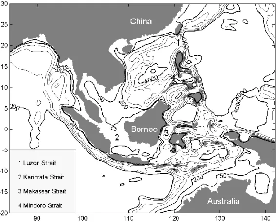
nutrients) from the Western Pacific to the Eastern Indian oceans (Figure 1). Most importantly, the 115
ITF transfers coupled modes of climate variability, such as El Nino-Southern Oscillation (ENSO). 116
The SCSTF and especially the ITF are subdivided into many pathways through both wide and 117
narrow straits separated by the numerous islands of the Indonesian Archipelago. For a review of 118
the ITF see Gordon (2005). Surface heat and moisture fluxes are especially important for the SCS 119
which gains heat from the atmosphere at a rate in the range 20 - 50 W/m2 per year and is also a 120
recipient of heavy rainfall with an annual mean value of 0.2 ~ 0.3 Sv (1 Sv=106 m3/s) over the 121
entire basin. On the long time average this heat and freshwater gain is balanced by horizontal 122
advection by the mean circulation. The cold, salty water of the western tropical Pacific entering 123
through the Luzon strait in the northern SCS is transformed into warm, fresh water exiting from 124
the southern Mindoro and Karimata straits. For a review of the SCS properties, see Qu et al. 125
(2009). In a word, this complex geometry, together with equally complex atmosphere-ocean 126
interactions, makes the modeling of the climate in this region a very challenging task. 127
7 / 39
2. Regional Atmospheric Model: RegCM3
129
Regional Climate Model (RegCM) was originally developed at the National Center for 130
Atmospheric Research (NCAR) and is now maintained by the International Center for Theoretical 131
Physics (ICTP). It is a three-dimensional, hydrostatic, compressible, primitive equation, σ-132
coordinate regional climate model. The dynamical core of RegCM Version 3 (RegCM3) is based 133
on the hydrostatic version of the Pennsylvania State University / NCAR Mesoscale Model 134
Version 5 (MM5; Grell et al. 1994) and employs NCAR’s Community Climate Model Version 3 135
(CCM3) atmospheric radiative transfer scheme (described in Kiehl et al. 1996). Planetary 136
boundary layer dynamics follow the non-local formulation of Holtslag et al. (1990; described in 137
Giorgi et al. 1993a). Ocean surface fluxes are handled by Zeng’s bulk aerodynamic ocean flux 138
parameterization scheme (Zeng et al. 1998). The Subgrid Explicit Moisture Scheme (SUBEX) is 139
used to handle large-scale, resolvable, non-convective clouds and precipitation (Pal et al. 2000). 140
Finally, three different convective parameterization schemes are available for representation of 141
non-resolvable rainfall processes (Giorgi et al. 1993b): Kuo (Anthes 1977), Grell (Grell 1993) 142
with Fritsch-Chappell (Fritsch and Chappell 1980) or Arakawa-Schubert (Grell et al. 1994) 143
closures, and Emanuel (Emanuel 1991; Emanuel and Zivkovic-Rothman 1999). Further details of 144
the developments and description of RegCM3 are available in Pal et al. (2007). 145
To represent the land surface physics, RegCM3 is coupled to the land surface scheme 146
Biosphere Atmosphere Transfer Scheme Version 1e (BATS1e; described in Dickinson et al. 147
1993). BATS1e uses a one-layer canopy with two soil layers and one snow layer to perform eight 148
major tasks, including: calculation of soil, snow or sea-ice temperature in response to net surface 149
heating, calculation of soil moisture, evaporation and surface and groundwater runoff, calculation 150
8 / 39
of the plant water budget, including foliage and stem water storage, intercepted precipitation and 151
transpiration, and calculation of foliage temperature in response to energy-balance requirements 152
and consequent fluxes from the foliage to canopy air (Dickinson et al. 1993). Additional 153
modifications have been made to BATS1e to account for the subgrid variability of topography and 154
land cover as described in Giorgi et al. (2003). 155
Winter et al. (2009) coupled RegCM3 to an additional land surface scheme – the 156
Integrated Biosphere Simulator (IBIS; described in Foley et al. 1996). IBIS uses a hierarchical, 157
modular structure to integrate a variety of terrestrial ecosystem phenomena. IBIS contains four 158
modules, operating at different time steps, and includes a two-layer canopy with six soil layers 159
and three snow layers. The four modules simulate processes associated with the land surface 160
(surface energy, water, carbon dioxide and momentum balance), vegetation phenology (winter-161
deciduous and drought-deciduous behavior of specific plant types in relation to seasonal climatic 162
conditions), carbon balance (annual carbon balance as a function of gross photosynthesis, 163
maintenance respiration and growth respiration), and vegetation dynamics (time-dependent 164
changes in vegetation cover resulting from changes in net primary productivity, carbon allocation, 165
biomass growth, mortality and biomass turnover for each plant functional type) (Foley et al. 166
1996). 167
168
3. Regional Ocean Model: FVCOM
169
FVCOM is a three dimensional, free surface, primitive equation, finite volume coastal 170
ocean model, originally developed by Chen et al. (2003). The model adopts a non-overlapping 171
unstructured (triangular) grid and finite volume method. The unstructured grid combines the 172
9 / 39
advantages of finite-element methods for geometric flexibility and finite-difference methods for 173
computational efficiency. FVCOM solves the momentum and thermodynamic equations using a 174
second order finite-volume flux discrete scheme that ensures mass conservation on the individual 175
control volumes and the entire computational domain (Chen et al., 2006a,b). The Mellor and 176
Yamada level 2.5 turbulent closure scheme is used for vertical eddy viscosity and diffusivity 177
(Mellor and Yamada, 1982) and the Smagorinsky turbulence closure for horizontal diffusivity 178
(Smagorinsky, 1963). The heat fluxes are assumed to occur at the ocean surface and the short 179
wave radiation penetrated into the water column is approximated following Simpson and Dickey 180
(1981). For details of FVCOM see http://fvcom.smast.umassd.edu/FVCOM/index.html. 181
In order to better represent the oceanic processes in the Southeast Asian region, the 182
flexible unstructured grid is capable of designing a model domain with varied resolutions 183
according to its complex geometry and topography. Our model domain covers the entire SCS, the 184
western Pacific and the eastern Indian Ocean (Figure 3), with two open boundaries at the Pacific 185
Ocean and the Indian Ocean respectively. This regional domain with open boundaries is chose to 186
be large enough to prevent possible boundary effects, such as spurious wave reflection, from 187
affecting the interior circulation. The grid contains 67,716 non-overlapping triangular cells and 188
34,985 nodes. The sigma coordinate is used in the vertical and is configured with 31 layers (finer 189
at surface and coarser at depth), which provides a vertical resolution of <1 m near surface on the 190
shelf, and about 10 m in the open ocean. The water depth at each grid point is interpolated from 191
ETOPO5 (Figure 1). The horizontal resolution is ~10 km along the coast of the islands of the 192
Indonesian Archipelago, ~50 km in the central SCS and ~200 km along the open boundaries. 193
For ocean-only simulations, such as during the spin-up phase, FVCOM is embedded with
194
one way coupling in the global ocean MITgcm (Hill and Marshall, 1995; Marshall et al., 1997) 195
10 / 39
which is a component of the MIT Integrated Earth System Model. The latter one comprises the 196
ocean GCM, a primitive equation, three-dimensional model with the resolution of 2.5o×2o and 22 197
vertical z-levels (layer thickness ranging from 10 m to 765 m). It includes a prognostic carbon 198
model. The atmosphere is represented by a statistical-dynamical two-dimensional (zonally 199
averaged) model with the resolution of 4o and 11 vertical z-levels. Land, sea-ice and an active 200
chemistry model are also included. Flux adjustment is also used by restoring the SST to 201
observations. A ―spreading‖ technique is used for the two-dimensional air-sea heat flux to 202
reconstruct the longitudinal dependence, i.e. dQ/dT*delta(T), where Q, latitude-dependent Q(y) 203
only, is the modeled calculated heat flux, and delta(T) is the difference of local temperature from 204
the zonal mean. Four decade simulations (60s-70s-80s-90s) are available from the MITgcm with 205
the full fields of currents, temperature, salinity and sea level. The atmospheric model provides the 206
surface heat and moisture fluxes. The wind stress however is given by the NCEP reanalysis with 207
6-hourly date for the entire period 1948-2000. The complex spin-up procedure of the MITgcm can 208
be found in http://mitgcm.org/public/r2_manual/latest/. 209
210
4. Coupling of RegCM3 and FVCOM
211
Here we developed a regional coupled atmosphere–ocean model in order to investigate the 212
climate over the Maritime Continent. The coupled model is developed using RegCM3 as the 213
atmospheric component and FVCOM as the oceanic component. The two models are coupled 214
using the OASIS3 software (http://www.cerfacs.fr/globc/software/oasis/oasis.html), which allows 215
flexible coupling for different model configurations and is suitable to run on massively parallel 216
computers. 217
11 / 39
In order to keep synchronization of RegCM3 and FVCOM, the two models are integrated
218
forward simultaneously and OASIS3 interpolates and transfers the coupling fields of different 219
resolution from the source grid to the target gird at a specified interval. At run time, RegCM3 and
220
FVCOM are respectively driven by lateral boundary forcing. In FVCOM, lateral forcing includes
221
SSH, temperature, and salinity along the open boundaries which are interpolated from simulations
222
of the MITgcm. In RegCM3, the lateral forcing includes temperature, winds, relative humidity
223
along the boundaries, interpolated from the European Centre for Medium-range Weather
224
Forecasts (ECMWF) 40-year Re-Analysis (ERA40) dataset (Uppala et al. 2005). The coupling
225
fields at the atmosphere-ocean interface were calculated in each model and exchanged through the
226
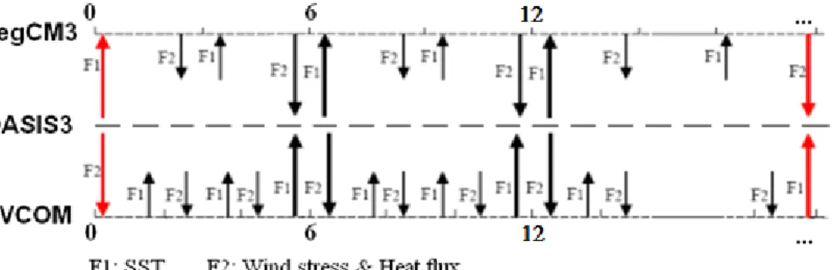
coupler, that is, RegCM3 supplies the solar heat fluxes, latent heat flux, sensible heat flux, surface 227
wind to FVCOM, and FVCOM provides SST for RegCM3. The timing of the exchange is shown 228
in Figure 2. While at each time step the coupler is automatically requesting the coupling fields 229
from the individual model, the exchange is actually taken place at every 6 hours, which is the 230
same frequency at which lateral boundary conditions are provided to the atmospheric model. The 231
details of the coupling process are described in the Appendix. 232
233
5. Results of Simulations using the Coupled Model
234
In order to investigate the decadal variability of climate over the Southeast Asian monsoon
235
region (Figure 1), the RegCM3-FVCOM coupled model was integrated for from 1960-1980 and
236
the results are validated with observations. The first decade simulation (60s) is for model spin-up
237
and the results of the second decade (70s) are summarized and presented.
238 239
12 / 39 5.1 Model spin-up (60s):
240
The coupled model was first spun up from 1960 to 1969. For RegCM3, the SST is
241
initialized with GISST data and then updated every 6 hours by SST obtained from FVCOM.
242
FVCOM started from rest condition with initial temperature and salinity from the MITgcm
243
simulation which is the first weekly average field of 1960. Figure 4 shows such the initial
244
condition for SST with the MITgcm resolution (2.5o×2o) evident. The temperature (salinity) at the
245
boundaries is relaxed to the temperature (salinity) of the MITgcm simulation. Heat fluxes were
246
updated every 6 hours from RegCM3. To establish a reasonable atmosphere-ocean interface
247
thermal structure a flux correction is used during the model spin-up for the decade of the 60s.
248
Specifically, the SST is relaxed towards the SODA SST analysis (Carton et. al 2000a,b) with a
249
depth dependent nudging factor, ranging from 0.2 s-1 in shallow water and decreasing to 0.001 s-1
250
in the open ocean. Thus in the open ocean the flux correction is negligible and the RegCM3 heat
251
fluxes dominate. In shallow water the flux correction dominates to keep the ocean model from
252
drifting from the climatology of the 60s. Furthermore, to obtain a stable reversal monsoon
253
circulation, sea level along the open boundaries at the Pacific and Indian Oceans is forced
254
perpetually by 10-year averages of weekly SSHA simulation from the MITgcm, and the surface
255
wind is gradually ramped up and updated every 6 hours from RegCM3.
256 257
5.2 Results of the 70s: 258
The simulation of the 70s was restarted from the model conditions saved at the end of the
259
60s. The model configuration of the 70s is the basically same as of the 60s except two changes.
13 / 39
First, differently from the spin-up phase, no flux correction is used in the simulation of the 70s,
261
hence in FVCOM relaxation of the SST to the observations is turned off. Second, the sea level at
262
open boundaries is driven by real time SSHA of the 70s.
263
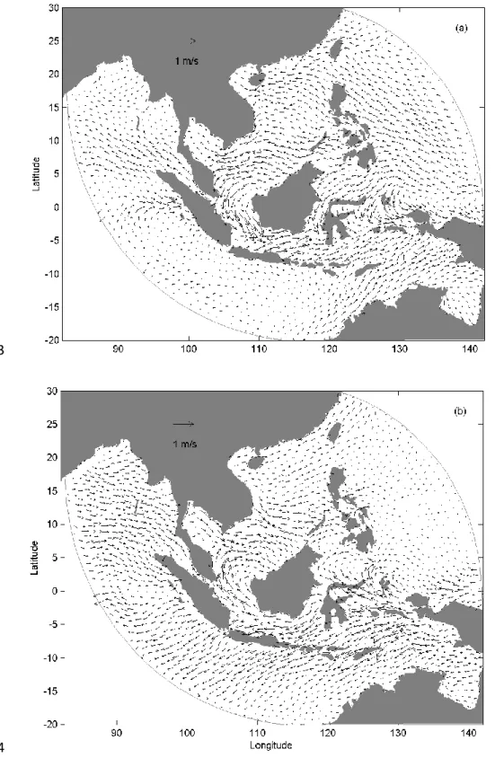
The Southeast Asian monsoon circulation, especially in the South China Sea, is driven by
264
surface wind and boundary sea level pressure gradient. Figure 5 show decadal average (70s)
265
surface circulations for winter (DJF) and summer (JJA) seasons. The coupled model successfully
266
reproduces the seasonal reversal of the SCSTF associated with the seasonality of the Southeast
267
Asian monsoon, North-Eastern in winter and South-Western in summer (Figure 6, also see Qu,
268
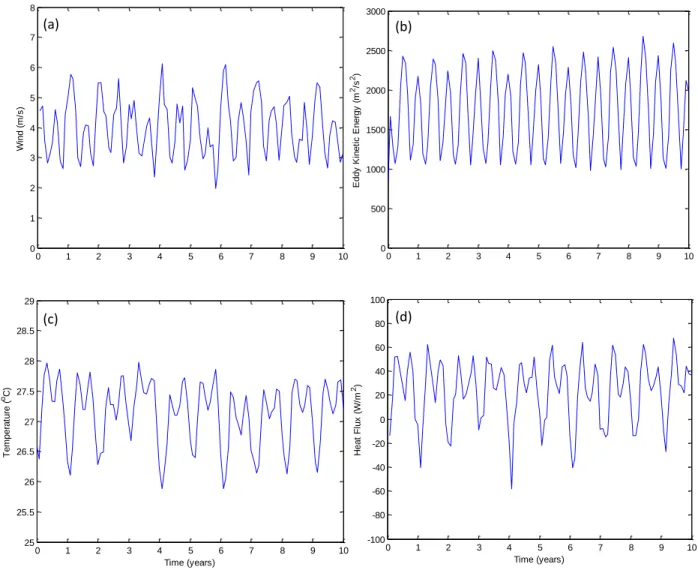
2000). Figures 7a-b show 10-year time series of domain average wind from RegCM3 and surface
269
eddy kinetic energy (EKE) from FVCOM. The wind speed clearly shows two peaks in each
270
annual cycle associated with the winter northeast monsoon and the summer southwest monsoon.
271
The surface EKE shows a very stable annual cycle throughout the 10-year simulation and is
272
highly correlated with the wind fluctuation, which implies the strong monsoon-driven
273
southwestward flow in winter and northeastward flow in summer (Figure 5). Similarly, the
274
domain average net heat flux also shows a clear cyclicity (Figure 7c). There are two maxima
275
occurred in summer when the incidence of the solar radiation is perpendicular to the earth equator
276
due to earth revolution. Since the SST relaxation is turned off, the ocean SST in the 70s
277
simulation is mainly driven by the heat fluxes as evident from Figure 7d.
278 279
5.3 Comparison with observations: 280
To assess the ability of the coupled model, here we compared the model results with
281
reanalysis and observations. Figure 8 compares the model simulations of SST, the SODA SST
14 / 39
reanalysis and their difference. The overall SST patterns show important similarities, with a band
283
of cold Pacific water protruding into the northern SCS and a band of warm water over the
284
Indonesian archipelago and the ITF in (boreal) winter. The SST pattern is reversed in summer.
285
However, the model SST is overall colder than SODA SST by 2 to 4 degrees (Fig. 8e-f), except
286
for the southern coast of China where the model SST is warmer than SODA SST in winter. We
287
remind that the initial condition for the coupled simulation represents the realistic SST at the end
288
of the 60s as in the spin-up phase the SST is relaxed to the SODA field. Therefore, during the
289
coupled simulation without the flux correction the ocean SST drifts away from the SODA
290
reanalysis producing a colder ocean. There are many possible reasons for this discrepancy, the
291
most plausible one being that the water masses continuously prescribed at the open boundaries
292
from the MITgcm do not provide a correct distribution of the water masses. In fact, Figure 8e-f
293
shows consistently rather colder waters all along the open model boundaries with respect to the
294
SODA reanalysis, both in winter and summer. This is particularly true for the entire western
295
Pacific and the Eastern Indian oceans in summer. As the major advective pathways are from the
296
Pacific to the Indian both through the SCSTF and the ITF, over 10 years the advection of rather
297
colder waters would affect the entire interior of the domain.
298
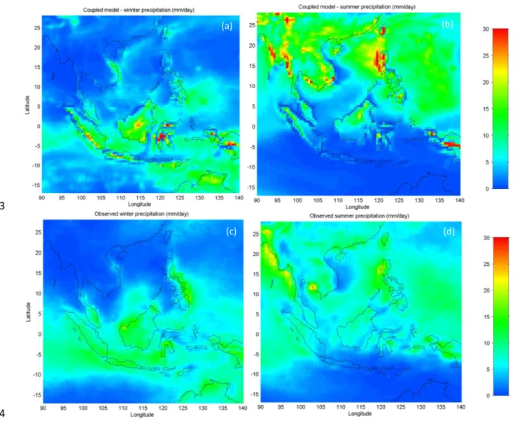
Figure 9 compares the seasonal precipitation of model simulation with TRMM
299
observations. In winter (DJF), the simulation is able to reproduce the basic climatology over the
300
domain, but with more precipitation over the maritime continent mountainous regions and less
301
precipitation over some oceanic areas of northern hemisphere. In summer (JJA), a systematic
302
overestimation of precipitation occurs in the northern hemisphere and underestimation is found in
303
the southern part of domain, associated with the passages of rain belts. Station-based comparisons
304
are showed in Figure 10. It can be seen that the model capture the annual cycles of precipitation at
15 / 39
Hong Kong and Darwin, with slightly more precipitation in dry season and obviously more
306
precipitation in wet season, suggesting that the extent of overestimation tends to relate the
307
movement of rain belts. Observed rainfall values highlight small differences at Singapore in each
308
month and similar characteristic is seen in the model simulation, but the somewhat higher values
309
from Oct. to Dec. in observation and lower values from Jun. to Aug. in simulation are actually
310
different enough to degrade our comparison. In general, the model can reproduce reasonably well
311
observed pattern of precipitation, despite it seemingly produces too much precipitation at the
312
monsoon rain belt, especially over the mountainous regions. These biases may be due to the
313
deficiency of the coupled model in producing more convective precipitation.
314
We also compare the simulated evaporation against the available observational TRMM
315
datasets (Figure 11). Generally evaporation is larger in cold season than in warm season over the
316
air-sea interface due to strong wind which is successfully captured in our model simulations.
317
Statistically discrepancies between simulations and observations are that the model exhibits
318
positive anomalies over the air-sea interface in both winter and summer, which may be one of the
319
reasons for the overestimation of precipitation.
320 321
6. Discussion, Summary, and Future Research
322
In order to investigate the regional climate over the Maritime Continent, this study
323
presents a newly-developed regional atmosphere-ocean coupled model. The coupled model adopts
324
RegCM3 as the atmospheric component and FVCOM as the oceanic component, using the
325
OASIS3 as the coupler. RegCM3 includes several options for representing important processes
326
such as moist convection and land surface physics. FVCOM features a flexible unstructured grid
16 / 39
that can match the complex geometries of the lands and the system of islands comprised in the
328
region as well as its complex topography. To keep synchronization of RegCM3 and FVCOM, the
329
two models are integrated forward simultaneously. At run time, RegCM3 and FVCOM are
330
respectively driven by lateral boundary forcing and OASIS3 interpolates and transfers the
331
coupling fields of different resolution between the two models. RegCM3 supplies the solar heat
332
fluxes, latent heat flux, sensible heat flux, surface wind to FVCOM, while FVCOM provides SST
333
for RegCM3.
334
The coupled model is developed and tested over the Southeast Asian Maritime Continent,
335
a region where a relatively shallow ocean occupies a significant fraction of the area and hence
336
atmosphere-ocean interactions are of particular importance. The coupled model simulates a stable
337
equilibrium climate over a decade (1970-1980) without the need for any artificial adjustments of
338
the fluxes between the ocean and the atmosphere. We compare the simulated fields of sea surface
339
temperature, surface wind, ocean currents and circulation, rainfall distribution, and evaporation
340
against observations. The coupled model reproduces an overall realistic pattern of SST, even
341
though colder than the SODA reanalysis, the major features of the monsoon circulation, as well as
342
rainfall and evaporation distributions over the region. The model results are in reasonable
343
agreement with the observed atmosphere/ocean climatology, suggesting that the coupled model
344
successfully captures the decadal variability of climate over this region. While differences
345
between simulations and observations are noted and will be the subject for further investigations,
346
the coupled model succeeds in simulating the main features of the regional climate over the
347
Maritime Continent including the seasonal north-south progression of the rainfall maxima and
348
associated reversal of the direction of the ocean currents and circulation driven by the surface
349
monsoons. The comparison with observations shows some differences over the mountainous
17 / 39
regions, especially for the rainfall simulation (Figure 9). These biases may be due to the
351
deficiency in the representation of clouds and moist convection. For the ocean component, the
352
discrepancies observed in the model SST, colder than the observed ones, may be due to an
353
incorrect representation of the water masses at the open ocean boundaries interpolated from the
354
MITgcm simulations. Our future research will focus on addressing some of the stated deficiencies
355
in the coupled model (e.g. wet bias in rainfall and cold biases in SST) and on investigating the
356
predictability of the regional climate system.
357 358
18 / 39
Appendix
359
The coupling process includes the following steps:
360
OASIS3 Configuration and Auxiliary Files: 361
OASIS3 needs configuration and auxiliary files configuring a particular coupled run, describing
362
coupling and I/O field names and units, defining the grids of the models, containing the field
363
coupling initial data values or restart data values, as well as a number of other auxiliary data files
364
used in specific transformations. The configuration file namecouple contains all users’ defined
365
information necessary to configure a particular run, such as the number of models being coupled,
366
the number of fields, coupling period, transformation and interpolation methods, etc. The text file
367
cf_name_table.txt contains a list of standard names and associated units identified with an index. 368
This information will be used by OASIS3 for its log messages to cplout file. In this study, we
369
configured two component models (RegCM3 and FVCOM) and 5 coupling fields (SST, solar heat
370
fluxes, non-solar heat fluxes, zonal wind and meridional wind).
371
Definition of Grid Data Files 372
Before running the coupled model, the coupler OASIS3 requires grid information of each
373
component model which can be created as netCDF files by users. The grid data files to be created
374
are grids.nc, mask.nc and areas.nc. grids.nc contains the component model grids, longitude and
375
latitude. The model grids can be any type of mesh, structured or unstructured. In this study, the
376
atmosphere model (RegCM3) used structured grid (rectangular grid) while the ocean model
377
(FVCOM) used unstructured grid (triangular grid). masks.nc contains the masks of atmosphere
19 / 39
and ocean for each component model. areas.nc contains mesh surfaces for the component model
379
grids.
380
Coupler Initialization 381
The subroutine inicma initializes and defines the variables returned by the coupler (SST) and
382
given to the coupler (solar heat fluxes, non-solar heat fluxes, zonal wind, meridional wind).
383
Sending the coupling fields: 384
This process is executed by calling the intocpl subroutine. RegCM3 supplies the solar heat fluxes
385
(short-wave and long-wave fluxes), non-solar heat fluxes (latent and sensible heat fluxes), zonal
386
wind (10 m) and meridian wind (10 m) and FVCOM supplies ocean SST to the coupler. While
387
this subroutine is called by each component model at each time step, the sending is actually
388
performed only if the time obtained by adding the fields lag to the argument date corresponds to
389
the time at which it should be activated.
390
Receiving the coupling fields: 391
This process is executed by calling the fromcpl subroutine. RegCM3 obtains SST and FVCOM
392
obtains solar and non-solar heat fluxes, and wind stress from the coupler. Similarly, the receiving
393
action is actually performed at the specific time at which it should be activated.
394
Transformations and Interpolations: 395
Different transformations and interpolations are available in OASIS3 to adapt the coupling fields
396
from the source model grid to the target model grid. In this study, we performed a time
397
transformation on all coupling fields, that is, before sending to the coupler, the coupling fields
20 / 39
were averaged over the previous coupling period. The interpolation techniques are from the
399
software of SCRIP (http://climate.acl.lanl.gov/software/SCRIP). A conservative remapping
400
scheme is used for solar and non-solar heat flux fields, which keeps the context fields conserved
401
over the area-integrated field. As for other fields (SST and wind stress), a method of
distance-402
weighted average of nearest-neighbor point interpolation is used.
403
Coupling restart file 404
When restart, the coupling fields have to be read from the coupling restart file on their source grid.
405
In our coupled model, the routine of prism_put_restart_proto writes restart fields at the beginning
406
of every month. The restart file is named flda.nc for RegCM3 and fldo.nc for FVCOM.
407
Termination 408
All processes must terminate the coupling by calling quitcpl subroutine. This will ensure a proper
409
termination of all processes in the coupled model communicator.
410 411
21 / 39
Acknowledgment
412
This study was supported by the Singapore National Research Foundation (NRF) through
413
the Singapore-MIT Alliance for Research and Technology (SMART) and Center for
414
Environmental Sensing and Monitoring (CENSAM) and by National Natural Science Foundation
415
of China (NSFC).
416 417 418
22 / 39
References
419
Aldrian E, Sein D, Jacob D, Du¨menil Gates L, Podzun R, 2005: Modeling Indonesian rainfall with a coupled
420
regional model. Clim Dyn 25:1–17
421
Anthes, R. A, 1977: A cumulus parameterization scheme utilizing a one-dimensional cloudmodel, Mon. Wea.
422
Rev., 105, 270-286.
423
Artale, V., Calmanti, S., and Carillo, A., et al., 2009: An atmosphere–ocean regional climate model for the
424
Mediterranean area: assessment of a present climate simulation. Clim Dyn, doi 10.1007/s00382-009-0691-8
425
Carton, J.A., G. Chepurin, X. Cao, and B.S. Giese, 2000a: A Simple Ocean Data Assimilation analysis of the
426
global upper ocean 1950-1995, Part 1: methodology, J. Phys. Oceanogr., 30, 294-309.
427
Carton, J.A., G. Chepurin, and X. Cao, 2000b: A Simple Ocean Data Assimilation analysis of the global upper
428
ocean 1950-1995 Part 2: results, J. Phys. Oceanogr., 30, 311-326.
429
Chen, C., H. Liu and R. C. Beardsley, 2003: An unstructured, finite-volume, three-dimensional, primitive
430
equation ocean model: application to coastal ocean and estuaries. J. Atmos. Oceanic Tech., 20, 159-186.
431
Chen, C., R.C. Beardsley, and G. Cowles, 2006a: An unstructured grid, finite-volume coastal ocean
model-432
FVCOM user manual, School for Marine Science and Technology, University of Massachusetts Dartmouth,
433
New Bedford, Second Edition. Technical Report SMAST/UMASSD-06-0602, 318pp.
434
Chen, C, R. C. Beardsley and G. Cowles, 2006b: An unstructured grid, finite-volume coastal ocean model
435
(FVCOM) system. Special Issue entitled ―Advance in Computational Oceanography‖, Oceanography,
436
19(1), 78-89.
437
Dickinson, R., A. Henderson-Sellers, and P. Kennedy, 1993: Biosphere Atmosphere Transfer Scheme (BATS)
438
version 1e as coupled to the NCAR Community Climate Model, NCAR Technical Note
NCAR/TN-439
387+STR, National Center for Atmospheric Research, Boulder, Colorado.
440
Döscher, R., U. Willén, C. Jones, A. Rutgersson, H. E. M. Meier, U. Hansson, and L. P. Graham, 2002: The
441
development of the regional coupled ocean–atmosphere model RCAO. Boreal Environ. Res., 7, 183–192.
23 / 39
Emanuel, K. A., 1991: A scheme for representing cumulus convection in large-scale models, J. Atmos. Sci.,
443
48(21), 2313-2335.
444
Emanuel, K. A., and M. Zivkovic-Rothman, 1999: Development and evaluation of a convection scheme for use
445
in climate models, J. Atmos. Sci., 56, 1766-1782.
446
Foley, J. A., I. C. Prentice, N. Ramankutty, S. Levis, D. Pollard, S. Sitch, and A. Haxeltine, 1996: An integrated
447
biosphere model of land surface processes, terrestrial carbon balance, and vegetation dynamics, Global
448
Biogeochem. Cycles, 10(4), 603-628.
449
Fritsch, J. M., and C. F. Chappell, 1980: Numerical prediction of convectively driven mesoscale pressure
450
systems. Part 1: Convective parameterization, J. Atmos. Sci., 37, 1722-1733.
451
Giorgi, F., M. R. Marinucci, and G. T. Bates, 1993a: Development of a second-generation regional climate
452
model (RegCM2). Part I: Boundary-layer and radiative transfer processes, Mon. Wea. Rev., 121,
2794-453
2813.
454
Giorgi, F., M. R. Marinucci, and G. T. Bates, 1993b: Development of a second-generation regional climate
455
model (RegCM2). Part II: Convective processes and assimilation of lateral boundary conditions, Mon. Wea.
456
Rev., 121, 2814-2832.
457
Giorgi, F., R. Francisco, and J. S. Pal, 2003: Effects of a sub-grid scale topography and land use scheme on the
458
simulation of surface climate and hydrology. Part I: Effects of temperature and water vapour
459
disaggregation, J. Hydrometeorol., 4, 317-333.
460
Gordon, et.al., 2005: Oceanography of the Indonesian seas and their through-flow. 18, 4, 14-27
461
Grell, G. A., 1993: Prognostic evaluation of assumptions used by cumulus parameterizations, Mon. Wea. Rev.,
462
121, 764-787.
463
Grell, G. A., J. Dudhia, and D. R. Stauffer, 1994: Description of the fifth generation Penn State/NCAR
464
Mesoscale Model (MM5), Technical Report TN-398+STR, National Center for Atmospheric Research,
465
Boulder, Colorado.
466
Gustafsson, N., L. Nyberg, and A. Omstedt, 1998: Coupling of a high-resolution atmospheric model and an
467
ocean model for the Baltic Sea. Mon. Wea. Rev., 126, 2822–2846.
24 / 39
Hagedorn, R., A. Lehmann, and D. Jacob, 2000: A coupled high resolution atmosphere–ocean model for the
469
BALTEX region. Meteor. Z., 9, 7–20.
470
Hill, C. and J. Marshall, 1995: Application of a Parallel Navier-Stokes Model to Ocean Circulation in Parallel
471
Computational Fluid Dynamics In Proceedings of Parallel Computational Fluid Dynamics:
472
Implementations and Results Using Parallel Computers, 545-552.
473
Holtslag, A. A. M., E. I. F. de Bruijn, and H.-L. Pan, 1990: A high-resolution air mass transformation model for
474
short-range weather forecasting, Mon. Wea. Rev., 118, 1561-1575.
475
Huang, B., P. S. Schopf, and J. Shukla, 2004: Intrinsic ocean–atmosphere variability of the tropical Atlantic
476
Ocean. J. Climate, 17, 2058–2077.
477
Kalnay, E., M.Kanamitsu et al., 1996: The NCEP/NCAR 40-year Reanalysis Project, Bull.Amer.Meteor.Soc.,
478
77,437-471
479
Kiehl, J. T., J. J. Hack, G. B. Bonan, B. A. Boville, B. P. Breigleb, D. L. Williamson, and P. J. Rasch, 1996:
480
Description of the NCAR Community Climate Model (CCM3), NCAR Technical Note TN-420+STR,
481
[Available online at: http://www.cgd.ucar.edu/cms/ccm3/TN-420/].
482
Li T, Zhou G Q., 2010, Preliminary results of a regional air-sea coupled model over East Asia. Chinese Sci Bull,
483
55, doi: 10.1007/s11434-010-0071-0
484
Loglisci, N., and Coauthors, 2004: Development of an atmosphere–ocean coupled model and its application
485
over the Adriatic Sea during a severe weather event of bora wind. J.Geophys. Res., 109, D01102,
486
doi:10.1029/2003JD003956.
487
Marshall, J., C. Hill, L. Perelman, and A. Adcroft, 1997: Hydrostatic, quasi-hydrostatic, and nonhydrostatic
488
ocean modeling. J. Geophys. Res., 102(C3), 5733-5752.
489
Mellor, G. L. and T. Yamada (1982), Development of a turbulence closure model for geophysical fluid problem.
490
Rev. Geophys. Space Phys., 20, 851-875.
491
Pal, J. S., and Coauthors, 2007: Regional climate modeling for the developing world: The ICTP RegCM3 and
492
RegCNET, Bull. Am. Meteorol. Soc., 88, 1395-1409.
25 / 39
Pal, J. S., E. E. Small, and E. A. B. Eltahir, 2000: Simulation of regional-scale water and energy budgets:
494
Representation of subgrid cloud and precipitation processes within RegCM, J. Geophys. Res. (Atmos.),
495
105(D24), 579-594.
496
Pullen, J., J. D. Doyle, and R. P. Signell, 2006: Two-way air–sea coupling: A study of the Adriatic. Mon. Wea.
497
Rev., 134, 1465–1483.
498
Qu, T. 2000: Upper-Layer Circulation in the South China Sea, J.Phys.Oceanogr., 30, 1450-1460
499
Qu, T., Y.T.Song and T.Yamagata, 2009: An introduction to the South China Sea through-floe: its dynamics,
500
variability and application for climate, Dyn.Atnos.Oceans, 47, 3-14
501
Ratnam JV, Giorgi F, Kaginalkar A, Cozzini S, 2008: Simulation of the Indian monsoon using the RegCM3–
502
ROMS regional coupled model. Clim Dyn. doi:10.1007/s00382-008-0433-3
503
Ren, X., and Y. Qian, 2005: A coupled regional air–sea model, its performances and climate drift in simulation
504
of the east Asian summer monsoon in 1998. Int. J. Climatol., 25, 679–692.
505
Schrum, C., U. Hübner, D. Jacob, and R. Podzun, 2003: A coupled atmosphere/ice/ocean model for the North
506
Sea and Baltic Sea. Climate Dyn., 21, 131–141.
507
Simpson, J. J. and T. D. Dickey, 1981: Alternative parameterizations of downward irradiation and their
508
dynamical significance. J. Phys. Oceanogr., 11, 876-882
509
Smagorinsky, J. (1963), General circulation experiments with the primitive equations, I. The basic experi-ment.
510
Mon. Wea. Rev., 91, 99–164.
511
Somot S, Sevault F, De´que´ M, Cre´pon M, 2008: 21st Century climate change scenario for the Mediterranean
512
using a coupled atmosphere-ocean regional climate model. Glob Planet Change 63(2–3):112–126
513
Uppala, S. M., and Coauthors, 2005: The ERA-40 Re-Analysis, Q. J. R. Meteorol. Soc., 131, 2961-3012.
514
[Dataset available online at: http://www.ecmwf.int/research/era/do/get/era-40]. Valcke S, Redler R, 2006:
515
OASIS3 User guide. PRISM support initiative report no 4, 60 pp
516
Xie, S.-P., and Coauthors, 2007: A regional ocean–atmosphere model for eastern Pacific climate: Toward
517
reducing tropical biases. J. Climate, 20: 1504—1522, doi: 10.1175/JCLI4080.1
26 / 39
Zeng, X., M. Zhao, and R. E. Dickinson, 1998: Intercomparison of bulk aerodynamic algorithms for the
519
computation of sea surface fluxes using TOGA COARE and TAO data, J. Climate., 11, 2628-2644.
520 521
27 / 39
List of Figures
522
Figure 1: RegCM3 domain and bathymetry with the 50, 200 and 4000 m isobaths shown as 523
thicker lines, and 1000, 2000 and 3000 m isobaths shown as thin lines. The major straits 524
are marked. 525
Figure 2: Schematic of RegCM3-OASIS3-FVCOM coupled model. The coupling fields (F1: SST; 526
F2: wind and heat fluxes) are exchanged every 6 hours. 527
Figure 3: FVCOM unstructured grids which contain 67,716 non-overlapping triangular cells and 528
34,985 nodes. 529
Figure 4: The weekly average of January 1st ~ 7th, 1960 from MITgcm simulations, which is used 530
as initial SST in the coupled model. The MITgcm SST has resolution of 2.5o×2o and 531
was interpolated to FVCOM grids. 532
Figure 5: 1970-1980 average surface circulations for (a) winter and (b) summer. The vectors 533
shown are extracted from FVCOM grid every 100 km. 534
Figure 6: 1970-1980 average net heat flux and wind speed for (a) winter and (b) summer. The 535
wind vectors shown are extracted from FVCOM grid every 50 km. 536
Figure 7: Time series (1970-1980) of domain average (a) wind speed, (b) eddy kinetic energy, (c) 537
SST and (d) net heat flux from 1970s simulations. Wind speed and net heat flux are 538
calculated in RegCM3, and eddy kinetic energy and SST are calculated in FVCOM. 539
Figure 8: Comparison of model simulations of SST (a-b), SODA SST reanalysis (c-d). The 540
differences (e-f) are calculated as (Model – SODA). 541
Figure 9: Comparison of precipitation between model simulations (1970s average) and TRMM 542
data (average of 1998~2011). (a) Model winter average precipitation, (b) Model 543
summer average precipitation, (c) Observed winter average precipitation and (d) 544
Observed summer average precipitation. 545
Figure 10: Comparison of annual cycle between observed and model precipitation at three 546
locations: Hong Kong, Singapore and Darwin. The observations and simulations are 547
spatial average within a 5o×5o box centered at the three locations respectively. 548
28 / 39
Figure 11: Comparison of evaporation between model simulations (1970s average) and TRMM 549
data (average of 1998~2011). (a) Model winter average evaporation, (b) Model 550
summer average evaporation, (c) Observed winter average evaporation and (d) 551
Observed summer average evaporation. 552
29 / 39 554
Figure 1: RegCM3 domain and bathymetry with the 50, 200 and 4000 m isobaths shown as 555
thicker lines, and 1000, 2000 and 3000 m isobaths shown as thin lines. The major straits are 556
marked. 557
558 559
30 / 39 560
Figure 2: Schematic of RegCM3-OASIS3-FVCOM coupled model. The coupling fields (F1: SST; 561
F2: wind and heat fluxes) are exchanged every 6 hours. 562
31 / 39 564
Figure 3: FVCOM unstructured grids which contain 67,716 non-overlapping triangular cells and 565
34,985 nodes. 566
32 / 39 568
Figure 4: The weekly average of January 1st ~ 7th, 1960 from MITgcm simulations, which is used 569
as initial SST in the coupled model. The MITgcm SST has resolution of 2.5o×2o and was 570
interpolated to FVCOM grids. 571
33 / 39 573
574
Figure 5: 10-year average surface circulations for (a) winter and (b) summer. The vectors shown 575
are extracted from FVCOM grid every 100 km. 576
34 / 39 577
578
Figure 6: 10-year average net heat flux and wind speed for (a) winter and (b) summer. The wind 579
vectors shown are extracted from FVCOM grid every 50 km. 580
581
(a)
35 / 39 582
583
Figure 7: Time series (1970-1980) of domain average (a) wind speed, (b) eddy kinetic energy, (c) 584
SST and (d) net heat flux from 1970s simulations. Wind speed and net heat flux are calculated in 585
RegCM3, and eddy kinetic energy and SST are calculated in FVCOM. 586 587 0 1 2 3 4 5 6 7 8 9 10 0 1 2 3 4 5 6 7 8 Time (years) W in d ( m /s ) 0 1 2 3 4 5 6 7 8 9 10 0 500 1000 1500 2000 2500 3000 Time (years) E d d y K in e ti c E n e rg y ( m 2/s 2) 0 1 2 3 4 5 6 7 8 9 10 25 25.5 26 26.5 27 27.5 28 28.5 29 Time (years) Te m p e ra tu re ( oC) 0 1 2 3 4 5 6 7 8 9 10 -100 -80 -60 -40 -20 0 20 40 60 80 100 Time (years) H e a t Fl u x ( W /m 2) (a) (b) (c) (d)
36 / 39 588
589
590
Figure 8: Comparison of model simulations of SST (a-b), SODA SST reanalysis (c-d). The 591
differences (e-f) are calculated as (Model – SODA). 592
(a) (b)
(c) (d)
37 / 39 593
594
Figure 9: Comparison of precipitation between model simulations (1970s average) and TRMM 595
data (average of 1998~2011). (a) Model winter average precipitation, (b) Model summer average 596
precipitation, (c) Observed winter average precipitation and (d) Observed summer average 597 precipitation. 598 599 (a) (b) (c) (d)
38 / 39 600
Figure 10: Comparison of annual cycle between observed and model precipitation at three 601
locations: Hong Kong, Singapore and Darwin. The observations and simulations are spatial 602
average within a 5o×5o box centered at the three locations respectively. 603 604 0 2 4 6 8 10 12 0 10 20 Precipitation (mm/day) H o n g K o n g 0 2 4 6 8 10 12 0 10 20 S in g a p o re 0 2 4 6 8 10 12 0 10 20 Time (months) D a rw in TRMM Model
39 / 39 605
606
Figure 11: Comparison of evaporation between model simulations (1970s average) and TRMM 607
data (average of 1998~2011). (a) Model winter average evaporation, (b) Model summer average 608
evaporation, (c) Observed winter average evaporation and (d) Observed summer average 609 evaporation. 610 611 (c) (a) (b) ) (a) (d) ) (a)