Cooperative multicast in wireless networks

Cooperative Multicast in Wireless Networks

by

Fulu Li

B.E., Computer Science, Southwest Jiaotong University (1994)

MSc., Computer Science, University of Alberta (2000)

Submitted to the Program of Media Arts and Sciences, School of Architecture and Planning,

In partial fulfillment of the requirement for the degree of MASTER OF SCIENCE IN MEDIA ARTS AND SCIENCES

at the

MASSACHUSETTS INSTITUTE OF TECHNOLOGY May 2005

0 Massachusetts Institute

Signature of Author

of Technology, 2005. All right reserved.

rogram in Media Arts and Sciences May 2, 2005 Certified by

Senior Research Sc' ntist of Ogram in

Andrew B. Lippman Media Arts and Sciences Media Arts and Sciences A Thesis Supervisor Accepted by

Andrew B. Lippman Chairman, Departmental Committee on Graduate Studies Program in Media Arts and Sciences

.ROTCH

JUN 27 2005

LIBRARIES

-Cooperative Multicast in Wireless Networks

by

Fulu Li

Submitted to the Program of Media Arts and Sciences, School of Architecture and Planning,

On May 2, 2005 in partial fulfillment of the requirement for the degree of

Master of Science in Media Arts and Sciences

Abstract

Wireless communication has fundamental impairments due to multi-path fading, attenuation, reflections, obstructions, and noise. More importantly, it has historically been designed to mimic a physical wire; in concept other communicators in the same region are viewed as crossed wires. Many systems overcome these limitations by either speaking more loudly, or subdividing the space to mimic the effect of a separate wire between each pair. This thesis will construct and test the value of a cooperative system where the routing and transmission are done together by using several of the radios in the space to help, rather than interfere. The novel element is wireless, cooperative multicast that could be the basis for a new broadcast distribution paradigm.

In the first part of the thesis, we investigate efficient ways to construct multicast trees by exploring cooperation among local radio nodes to increase throughput and conserve energy (or battery power), whereby we assume single transmitting node is engaged in a one-to-one or one-to-many transmission. In the second part of the thesis. we further investigate transmit diversity in the general context of cooperative routing. whereby multiple nodes are allowed for cooperative transmissions. Essentially, the techniques presented in the second part of the thesis can be further incorporated in the construction of multicast trees presented in the first part.

Thesis Supervisor: Andrew B. Lippman

Cooperative Multicast in Wireless Networks

by

Fulu Li

A

Thesis Reader:

David P. Reed Adjunct Professor of Media Arts and Sciences

/ "f-ssachusetts Institute of Technology

Thesis Reader:

Philip J. Fleming Motorola Scientist - in-Residence Fellow of the Technical Staff

Acknowledgements

I would like to thank my advisor Dr Andrew B. Lippman for his mentorship and tremendous support. I greatly appreciate his openness, challenge and understanding, which made my research at MIT enjoyable. I would like to thank Dr David P. Reed for his technical insights and encouragement, which have always been a great source of motivation for my work. I feel

lucky to have the opportunity to know him and to interact with him. I would like to thank Dr Philip J. Fleming for his assistance, friendship and constructive comments on all aspects of my research. His candid advice is a great source of inspiration for my research.

My friends and colleagues at MIT made the last two years memorable: Xin, Wei, Jamie, Hector, Kwan, Aggelos, Xu, Xiaohua, Victor, Brian. John. Shie and all other people I have come to know in the US.

I would also like to thank my parents, my brothers, my sister and my wife, Jing Gao, whose support I enjoyed throughout the years.

Table of Contents

I

2 Cooperative Multicast in Wireless Networks 12

2.1 T he O verview ... 12

2.2 The Related Work...14

2.3 T he System M odel...17

2.4 Power Consumption Rules...17

2.5 Combining Existing Approaches...19

2.5.1 BIP+IMBM vs BIP ... 21

2.5.2 MST+IMBM vs MST ... 22

2.6 The RTO Algorithm ... 23

2.6.1 Random Tree Generation ... 25

2.6.2 Speedup of Random Tree Generation Algorithm ... 25

2.6.3 Exploitation of WBA ... 26

2.6.4 The Criticality of Randomness ... 26

2.6.5 The RTO Algorithm ... 29

2.6.6 Speedup of the RTO Process... 29

2.7 Performance Evaluation ... 30

3

Cooperative Routing in Wireless Networks

42

3.2.1 The Nctwork Model .48

3.2.2 The Power Consumption Model .48

3.3 The MECP Problem .51

3.4 Complexity Issues .. .54

3.5 Cooperative Shortest Path Algorithm ..62

3.5.1 CSP with Additive Constraints .... 67

3.5.2 Exploiting the first-hop WMA 69

3.6 Performance Evaluation .72

3.7 Distribution and Implementation Issues .91

4 Prototype Implementation 93

4.1 Hardware Components ...93

4.2 Software Components 94

5 Conclusion 98

List of Figures

Fig. 2-1 Evolving of Transition Probability Matrix 32

Fig. 2-2 RTO vs BIP and MST with Adaptive Matrix Initialization, 2=2 38 Fig. 2-3 RTO vs BIP and MST with Equal-Probability Initialization, 2=2 ..39

Fig. 2-4 RTO vs BIP and MST, 2=3 .40

Fig. 2-5 RTO vs BIP and MST, 2=4 .41

Fig. 3-1 Cooperative Transmissions with L=2 ..52

Fig. 3-2 An Example Path ... 56

Fig. 3-3 New Relaxation Procedure for CSP Algorithm .64

Fig. 3-4 An Example Run by CSP, CAN and PC 66

Fig. 3-5 New Relaxation Procedure for CSP Algorithm with Constraints ..68 Fig. 3-6 CSP vs CAN and USP in terms of Energy Efficiency ... 76

Fig. 3-7 CSP vs CAN and USP in terms of Fairness ..83

Fig. 3-8 CSP vs CAN and USP in terms of total Required Energy .89 Fig. 4-1 Snapshot of Prototype Implementation ..95

Fig. 4-2 Snapshot of Prototype Implementation ..96

List of Tables

Table 2-1 BIP+IMBM vs BIP ... 21

Table 2-2 MST+IMBM vs MST ... 22

Table 2-3 R TO vs B IP ... 30

T able 2-4 R T O vs M ST ... 31

Table 2-5 RTO vs BIP and MST, a = 0.8 ... 35

Table 2-6 RTO vs BIP and MST, a = 0.7 ... 36

Table 3-1 STD of normalized path power by CAN and USP, L =2 ... 81

Table 3-2 STD of normalized path power by CAN and USP, L =3 ... 81

Table 3-3 STD of normalized path power by CAN and USP, L =4 ... 82

Chapter 1

Introduction

Wireless communication has fundamental impairments due to multi-path fading, attenuation, reflections, obstructions, and noise. More importantly, it has historically been designed to

mimic a physical wire; in concept other communicators in the same region are viewed as crossed wires. Many systems overcome these limitations by either speaking more loudly, or subdividing the space to mimic the effect of a separate wire between each pair. This thesis will construct and test the value of a cooperative system where the routing and transmission are done together by using several of the radios in the space to help, rather than interfere.

In the first part of the thesis, we investigate efficient ways to construct multicast trees by exploring cooperation among local radio nodes to increase throughput and conserve energy

(or battery power), whereby we assume single transmitting node is engaged in a one-to-one or one-to-many transmission. In the second part of the thesis, we further investigate transmit diversity in the general context of cooperative routing, whereby multiple nodes are allowed for cooperative transmissions. Essentially, the techniques presented in the second part of the thesis can be further incorporated in the construction of multicast trees presented in the first part. We determine this as one of our future directions.

The motivation of this work is two-fold. The first is the importance of energy efficiency: a portable radio system's utility for many applications is dependent on how long the battery can

last. This is a basic design parameter for military, sensor and consumer networks. We often conserve energy by circuit design and operation (for example, see [4]. where clock speed is varied to save power.) Others use multiple antennas (diversity) [101 to conserve radiated power. We will explore cooperation, where multiple nodes join in transmission to achieve similar savings as diversity.

The second motivation is scalability. In large and dense wireless networks, transmitting with excessive power on one link leads to interference with other receivers. This limits the throughput of the network -- more radios do not result in more communications. Multi-hop networks [1,2,5,7,9,12,13,15-20,25,28,30-33] reduce the power at each node, and thereby limit the spurious radiation in the space. This can help the network scale.

In the first part of this thesis, we extend the notions of cooperative distribution for the sake of energy efficiency to situations where the data is shared among many subscribers. The assumption has always been wireless point-to-point communications 113,25,28,33]. We show the utility and benefits of cooperation for broadcast and multicast applications in this thesis. More specifically, we present a random tree optimization approach that transforms the deterministic optimization problem of wireless multicast into a related stochastic one. We apply the cross-entropy method [8,27] to this problem. Preliminary results show that it achieves considerable power savings compared with state-of-the-art approaches.

Please note that we assume single transmitting node is engaged in a one or one-to-many transmission in the construction of multicast trees in the first part of this thesis. In the second part of this thesis, we explore transmit diversity in the context of cooperative routing

where multiple nodes are allowed for cooperative transmissions. The Viral Communications group at MIT Media Lab pioneered the idea of multiple antenna radio systems, where the various antennas were on different nodes in a network, versus being fed from one source and physically distributed. Recently, others have also explored this idea. For example, Khandani et al in 113] showed that such cooperative transmission, where more than one node adds energy to a transmission saves overall energy. We improved on that to show further power savings with a simpler architecture. This is another essential component of this thesis. First, we prove the NP-hardness of the minimum energy cooperative path problem. We then present a cooperative shortest path algorithm to approximate the minimum energy cooperative path. The empirical results indicate that the presented approach tends to make the network more scalable and more efficient compared with existing approaches from both the

energy conservation and fairness standpoints.

As mentioned before, the techniques presented in the second part of the thesis can be further incorporated in the schemes for the construction of cooperative multicast trees presented in the first part of the thesis. We determine this as one of our future directions.

Chapter 2

Cooperative Multicast in Wireless Networks

2.1

The Overview

Wireless communication is becoming increasingly important for both voice applications and

data applications. Wireless networks are burgeoning at virtually every corner of the World.

In particular, a wide range of mission-critical applications have been developed for

all-wireless networks, such as battlefield operations for military missions, an emergency relief

for terrorist-based biochemical attacks, monitoring of the live images of multiple

condition-critical patients by the doctor using hand-held devices while away from the patients, etc. A

description of such an all-wireless network was given by Cagalj et al in Il1, and basically it

consists of numerous devices (also referred as nodes throughout this thesis) that are equipped

with processing, memory, wireless communication capabilities, and are linked via

short-range ad-hoc radio connections.

Notably, the lifetime of a wireless network is limited due to the power capacity of the energy

sources such as batteries. The lifetime of such a wireless network depends on the energy

consumption of each node. To increase the longevity of such networks, power-efficient and

power-aware protocols and techniques including link layer, MAC, routing and transport

protocols must be employed to minimize the power consumption (we will use energy and

In this chapter, we focus on the construction of the energy-efficient broadcast tree. The broadcast tree is rooted at the source and should reach all of the desired destination nodes. Following [321, we consider a wireless ad-hoc network in which the node locations are fixed and the channel conditions are unchanged. The situation with the mobility of the nodes in the construction of broadcast tree can be addressed by adjusting the transmitter power to accommodate the new locations of the nodes, which is a topic for future studies. We also assume that the power level of a transmission can be chosen within a given range of values and the use of omni-directional antennas. Thus, all nodes within communication range of a transmitting node can receive its transmission.

Moreover, we assume that sufficient bandwidth resources and ample transceiver resources are available at each node. The energy consumption between the transmitting node and the receiving node is not linear because of the nonlinear attenuation properties of radio signals. Due to the non-linear path loss model of the transmission power, relaying information between nodes may lead to lower power attenuation than communication directly over large distances.

In this thesis, we explore performance improvement by applying the iterative maximum-branch minimization (IMBM) approach [15] to other existing schemes and the empirical results show that considerable power savings can be achieved in particular when the value of the power attenuation factor A is small.

Our major contribution is the presentation of the random tree optimization (RTO) approach, which is based on the cros s-entropy method 18,27]. The basic idea behind the cross entropy method is to translate the deterministic optimization problem into a related stochastic optimization problem by randomly generating improved sample trees and then use rare event simulation techniques to find the solution. We will show that the RTO method obtains the best performance comparing to state-of-the-art heuristics for the MEB problem.

The rest of this chapter is organized as follows. We discuss related work in Section 2.2. We give the system model in Section 2.3. The power consumption rules are given in Seciton 2.4. We explore further power savings by combining some of the existing schemes in Section 2.5. We present the RTO algorithm in Section 2.6. The experimental results are presented in Section 2.7.

2.2

The Related Work

The multicasting problem in wireless networks has been addressed in several recent studies 11,7,15-20,23,24,30,321. In particular, 11,7,15-19,30,32] addressed the construction of energy-efficient broadcast and multicast trees in wireless networks. Several interesting heuristics were proposed in 1321, which can be roughly divided into two categories: link-based approaches and node-link-based approaches. As the names suggest, link link-based approaches, the BLU (Broadcast Least-Unicast-cost) algorithm and the MST (broadcast link-based Minimum-cost Spanning Tree) algorithm, use the link-based costs and further the shortest unicast paths and spanning trees. The node-based approach, i.e., the BIP (Broadcast Incremental Power) algorithm, constructs the broadcast tree incrementally in the sense that

new nodes are added to the tree one at a time on a minimum incremental cost basis until all nodes are included in the tree. Compared with the link-based approaches, BIP better exploits the wireless multicast advantage in the construction of the broadcast tree and demonstrates better performance than BLU and MST [32]. However, due to the incremental nature of BIP, it lacks a global view of all the nodes and it can not fully utilize the wireless broadcast advantage to reduce the total required power of the broadcast tree further. In [301, Wan et al presents a quantitative and in-depth analysis on the approximation ratios of the heuristics presented in 132].

In [151, Li et al proved that the MEB problem is NP-hard for the general case. Most recently, Cagalj et al in [1 presented a systematic and elegant proof on the NP-completeness of the MEB problem both for the general case and for the geometric one. A heuristic called EWMA (Embedding Wireless Multicast Advantage) was also suggested in I11. In EWMA, a distributed MST (Minimum-Spanning Tree) algorithm is executed in the first phase to obtain a feasible broadcast tree. In the second phase of EWMA, the so-called local EWMA is executed at each node in order to exclude some transmitting node from its neighbors to reduce the total required power of the tree by broadcasting or re-broadcasting messages based upon the calculation of the overlapping set for a sender.

An Iterative Maximum-Branch Minimization (IMBM) algorithm is proposed in 115] for the construction of energy-efficient broadcast trees. The algorithm assumes an initial tree and tries to minimize the required power for each transmitting node iteratively by minimizing its

maximum branch using wireless broadcast advantage until the total required power for the

broadcast tree can not be reduced further.

Das et al in 17] presented several different integer programming formulations of Minimum

Power Broadcast (MPB) trees for wireless networks in order to achieve the optimal solution.

The number of variables and constraints are at least in the order of O(N 2), where N is the

number of nodes in the network. The basic idea is to solve a linear relaxation of the problem

first, if the solution is integer, then the algorithm terminates with an optimal solution. If the

solution is not an integer it creates two sub-problems and branches down on a fractional

variable until no active sub-problem exists any more. The downside of this approach is that

problems with as few as 100 nodes can be practically intractable unless they demonstrate

some simplified structures.

Other researchers also address the power efficiency issue in the areas of distributed topology

control and wireless sensor networks. Rodoplu and Meng [26] proposed a novel distributed

position-based network protocol to achieve the minimum-energy network topology.

Wattenhofer et al [31] presented an ingenious distributed topology control algorithm for

power efficiency in wireless ad-hoc networks based on directional information. In 112],

Heinzelman et al proposed a cluster-based protocol to randomly rotate the local cluster base

stations to evenly distribute the energy consumption in wireless sensor networks.

In Section 2.6, we propose the Random Tree Optimization (RTO) approach based on the

Our experimental results in Section VI indicate that the RTO method achieves the best results

comparing to other methods.

2.3

The System Model

We consider an all-wireless network where numerous devices, i.e., nodes, that are equipped

with micro-processor, memory, sufficient bandwidth and transceiver resources, limited

power supply such as batteries are linked via short-range radio connections. We study the

problem of source-initiated broadcast through which data are disseminated to each of the.

intended destination node in the network. As stated in Section I, we assume the use of

omni-directional antennas and all nodes within communication range of a transmitting node can

receive its transmission.

As pointed out in [22], the communication power includes several components such as the

path loss, i.e., the power attenuation over the distance between the transmitter and receiver

antennas, the start-up energy of the transceiver, the static power drawn by the transmitter and

receiver electronics, power amplifier inefficiencies, coding energy and protocol overhead.

Following [1,7,13,15-19,28,30,32], we only consider the path loss as the dominant factor of

the communication power and most of the other components are static and

hardware-dependent and can be easily incorporated in the protocol design.

It is well known that the path loss of the signal power is non-linear. We assume that the required power for a range of d between the transmitting node and the receiving node is proportional to d A. Typically, A takes a value between 2 and 4, depending on the characteristics of the communication medium. We assume that the communication medium is uniform, thus A is a constant throughout the region. Given a source node S and destination nodes D,, D,,..., D1,, we want to establish a broadcast tree, rooted at node S and reaching all of the destination nodes, with the least required energy.

Regarding the transmission energy, we have the following definitions:

Definition 2.1: The power required for a transmitting node, say T, to directly reach a set of destination nodes, say D, D,,..., Di, is determined by the maximum required power to reach

any of them individually. For the sake of brevity, throughout this thesis we will use d^ to stand for the required power for a transmitting distance of d . Let d ,,,...,d,, stand for the

distances from the transmitting node T to the destinations D1, D, Dm, respectively. The

required power is determined by:

p = max(dF n , d,..., d,;) . (2.1)

Definition 2.2: The power required for a broadcast tree is the sum of the energy required for each of the transmitting nodes in the tree. Let S, T,,T 2,...,T, stand for the transmitting nodes

Let psPr,,-P p7 denote the required power for the transmitting nodes S,T,T,...,T,

respectively. The required power for the given broadcast tree is given by:

Pree = ps +( P,; (2.2)

The problem can be stated as how to construct a broadcast tree such that the total required energy is minimal.

According to Cayley 131, there are n"n2 _{distinct labeled free trees on n vertices. For if X is a}

particular vertex, the free trees are in one-to-one correspondence with oriented trees having root X [141. Therefore, for the case with the root node S and N destination nodes, we have

(N + 1)(N-'distinct labeled free trees.

In summary, the general MEB optimization problem is a difficult problem due to the fact that (a) the problem is combinatorial and NP-hard; (b) the cost function is non-linear, i.e., di for the required transmitting power from node i to node

j

As the IMBM approach 1151 assumes an initial tree, an interesting direction is to apply this approach to the broadcast trees generated by other existing algorithms to further minimize the required tree power. In the following experiments, we evaluate the impact of the IMBM algorithm on other existing approaches if we apply IMBM to the trees generated by other approaches. We use the same simulation setup as in [321. We consider many randomly-generated network examples (50 instances for each round of simulations), in which a specified number of nodes are randomly generated within a square region, say 5x5, the location of each node is randomly generated and the source node is randomly selected among the randomly-generated nodes. For the clarity and simplicity of the comparison, we use the same assumption as that in 132] that each node has enough power to cover all the other nodes and the power level of each node can be adjusted within a given range. We also consider the propagation loss exponents of A =2, A = 3, and A = 4 in our experiments. For the performance comparison between the algorithms, we consider normalized tree power. For example, suppose we have three approaches to generate broadcast trees. say approaches A, B and C. Let p, , p,, and p(. stand for the required tree power for the trees generated by approaches A, B and C, respectively for the same network topology. The normalized tree power for each of these approaches is given by the following:

* PA min(pA, _{PB' pc)} * P/1 PB _min(pA, p P _PC) PC = ( .I (2.3) minl( p." ,7 pPC)

As reported in [32], the performance of BLU approach is always much worse than BIP and MST. We therefore only examine the impact of IMBM on BIP and MST.

2.5.1 BIP+IMBM vs BIP

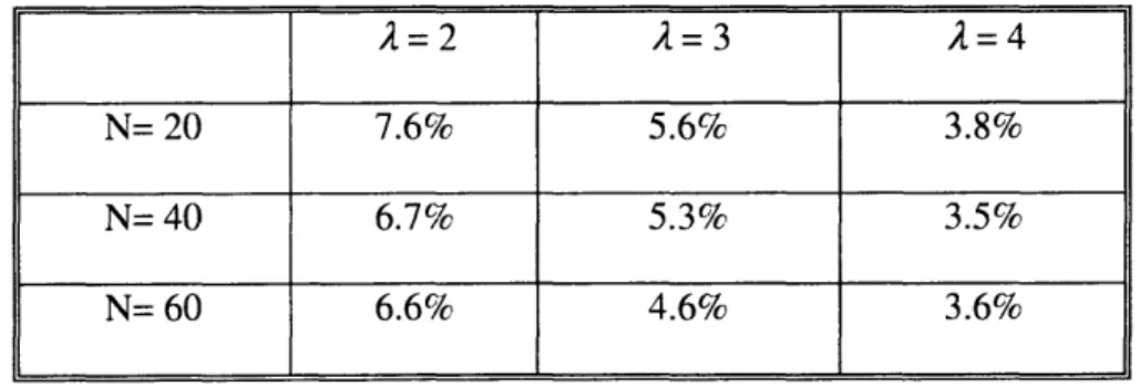
Table 2-1 shows the performance comparison between BIP+IMBM and BIP in a variety of circumstance, e.g., networks with different number of nodes (N = 20,40,60) and different power attenuation factor values (A = 2,3,4). The average tree power decrement ratio after the application of IMBM to the trees generated by BIP ranges from 3.5% to 7.6% for each round of the experiments. We can also observe that the decrement ratio of the tree power after the application of IMBM slightly shrinks with the increasing of the A value. The same trend holds with the increase of network density. This suggests that the incremental approaches like BIP works well for the networks with high node-density in fast power attenuation environments.

Table 2-1: Average decrement ratio of the normalized tree power after applying IMBM to the broadcast trees generated by BIP (50 randomly-generated network instances for each group).

A=2 A=3 A=4

N= 20 7.6% 5.6% 3.8%

N= 40 6.7% 5.3% 3.5%

2.5.2 MST+IMBM vs MST

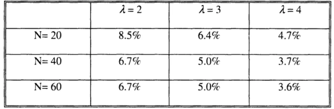
Table 2-2 depicts the performance comparison for MST+IMBM versus MST in the same settings as above. The average tree power decrement ratio after the application of IMBM to the broadcast trees generated by MST ranges from 3.5% to 8.6%, depending on the network densities and A values for each round of the experiments. Similarly, we can observe that the

decrement ratio of the tree power slightly shrinks with the increasing of the A value, the

increasing of the network density. Again, this suggests that both MST and BIP work well in a

network with high node-density in fast power attenuation environments.

Table 2-2: Average decrement broadcast trees generated by

group).

ratio of the normalized tree power after applying IMBM to the

MST (50 randomly-generated network instances for each

In summary, the key findings are: (a) IMBM consistently improves the performance of the existing approaches like MST and BIP after the application of IMBM to the broadcast trees generated by these existing approaches. (b) IMBM's impact varies with different network

densities and different A values in both cases.

A=2 A=3 2=4

N= 20 8.5% 6.4% 4.7%

N= 40 6.7% 5.0% 3.7%

2.6

The RTO Algorithm

As we discussed in Section 11, although the integer programming approach 171 can solve small-sized problems exactly, it will run into problems when the number of nodes in the network becomes large. For example, even when the number of nodes in the network greater than 10, the number of variables and constraints according to the Integer Programming (IP) formulations presented in [71 are both greater than 100, which is beyond the abilities of even the most powerful computers today. The Cross Entropy (CE) method, (see, e.g., Rubinstein et al [8,27]) is a useful meta-heuristic optimization method for finding near-optimal solutions in a variety of combinatorial optimization problems. The basic idea is to translate the deterministic optimization problem into a related stochastic optimization one and then use Rare Event Simulation (RES) techniques to find the solution.

We call the specification of the CE method to MEB problem the Random Tree Optimization (RTO) algorithm. We will see in the following that the algorithm operates iteratively by randomly generating improved sample trees until the optimization process converges based on our predefined performance function, i.e., the total required power of the tree.

First, we define the performance function F(tree) as the total required power of a tree, which is given according Definition 2.2 (see Equation 2.2). There are two key components in the RTO process based on CE: (1) Generation of random sample trees; (2) Update of the parameters at each iteration. The update mechanism is supposed to encourage trees with high

performance so that the randomization mechanism would lead to trees with even better performance.

We use a Markov chain that starts at the root node and stops after all of the destination nodes are reached to construct a sample tree. We define

Q=(q,

to node

j.

In order to find local neighbors first to avoid some "far-reached" transmissions to dominate the total required power of the tree, which could potentially degrade the performance of the RTO optimization process, the initial transition matrix Q can be set as follows: (a) the column corresponding to transmissions to the root node in the matrix and the diagonal elements are set to zero as no node transmits to itself and no node transmits to the root node; (b) for other elements qj1, we have

-/(dJ + c) (24

q,.j (2.4)

J (d,, +c)

where cis a constant that is related to the diameter of the network. When cis zero, the transition probability q,1 is solely determined by the distance between node i and node

j.

When c is much bigger than the diameter of the network, the transition probabilities in each column of the matrix are almost uniform. We will discuss this issue further in section VI.

In the following, we give a brief description of the random tree generation algorithm:

2.6.1 Random Tree Generation for RTO

The Random Tree Generation Algorithm: 1. Let I= 1.

2. Randomly choose a non-root node from the non-parented nodes (nodes who do not have parent node yet), say node ni, then randomly choose a parent node for node ni from its

non-descendent nodes (nodes who are not under n, s hierarchy) based on the transition probabilities given in the matrix

Q.

3. If 1 = N -1 then stop; otherwise set =1 + I and reiterate from step 2.

2.6.2 Speedup of the Random Tree Generation Algorithm

We use N -bit bitmap array for each node to indicate the ancestor-descendent relationship. During the tree generation process, when finding a parent node for a given node, we set this parent node and the parent node's ancestors as this given node's ancestors. It should be noted that when a given node's ancestors are updated, all of this node's descendents also need to inherit its updated ancestors. When checking the ancestor-descendent relationship to find a random parent node, it is faster to do so by directly examining the value of the bitmap array

instead of a recursive search. The complexity of the resulted random tree generation algorithm is in the order of O(N 3), where N is the number of nodes in the network.

2.6.3 Exploitation of Wireless Broadcast Advantage

During the process of the random selection of a parent node for a given node in random tree generation algorithm, we use a procedure called RandomFreeParent( ) to check that if there are some transmitting nodes in the current structure such that the given node is located in their coverage area. We call the nodes whose transmissions already covers a node the node's free parent as it does not need any additional power consumption by randomly choosing one of them to fully exploit the wireless broadcast advantage (WBA). If no free parent node can be found for this given node, we randomly choose one of its non-descendent nodes as its parent node based on the transition probability matrix.

2.6.4 The Criticality of Randomness

The randomness of the tree generation procedure is the key to the effectiveness and efficiency of the RTO algorithm. For example. we can have a seemingly random tree generation algorithm as follows:

1. Let 1= 1 and include the root node only as the initial tree.

2. Randomly choose a node that is not yet included in the tree, say node n,, then randomly choose a parent node for node ni from those nodes that are already included in the tree based on the transition probabilities given in the matrix

Q.

3. If I = N - I then stop; otherwise set 1 = I + I and reiterate from step 2.

Experimentally, we found that this seemingly random tree generation procedure leads to severely degraded performance of an RTO algorithm because this tree generation algorithm is not perfectly random as it gives biased priority to the root node.

We now turn our attention to the update algorithm. At each iteration of the RTO algorithm based on the CE method, we need to calculate the benchmark value of 7, as follows:

7, = min{f :

Q_,

f)

where p normally takes a value of 0.01 so that the event of obtaining high performance is not too rare, F(T) stand for the total required power of a randomly-generated sample tree, say

T, based on the one-step transmission probability matrix in the (t - 1)'" round, e.g.,

Q,

P (A) denote the probability of the event A conditioned on

Q,

There are several choices to set the termination conditions. Normally, If for some t 1, say

1= 5,

(2.6) 7, = 7,_1 =... = 7,_ ,

The updated value of qi .* can be estimated as: HH 7E {'H I Fi A )!5 7 qk= (2.7)

where M stands for the number of sample trees, H, is an indicator function, T. denotes the set of trees in which there is a transmission from node i to node

j.

q,, a x q=x +(1-a)xq', (2.8)

where q is the value of qi1 in the previous round and q'. is the estimated value of q

based on the performance in the previous round according to Equation (2.7), and q1 stands

for the value of qi, for the current round. Empirically, a value of a between 0.4 a 0.9 gives the best results 127].

2.6.5 RTO Algorithm based on Cross-Entropy (CE) method

1. Set t = 1 and set

Q)

3. Calculate 7, according to Equation (2.5).

4. Update q according to Equation (2.7) and Equation (2.8).

5. If for some t 2l, say I= 5, such that , == 7, ,_,, then stop; otherwise, reiterate

from step 2.

2.6.6 Speedup of the RTO process

As discussed before, the complexity of the random tree generation algorithm is in the order

of O(N') and normally we generate 2ON2sample trees for each round. Therefore, the

overall computation complexity of the RTO algorithm is in the order of O(N). For a large

value of N, the RTO process could be slow. We use the following strategies to speed up the

RTO algorithm: (a) Ignore small transition probabilities, say for qj1 <0.01, we force them to

be zero and renormalize it for each column of the transition probability matrix. (b) Set a

looser termination criterion. Normally, we set I = 5 for the termination condition according to

Step 5 of the RTO algorithm. When N is large, we opted to set 1 = 2 instead, and we use a

fast localized greedy routine to further optimize the tree generated by RTO.

In the following section we present extensive experiments that evaluate the performance of

2.7

Performance Evaluation

Following similar assumptions and settings in Section 2.5, we examine the dynamics of the RTO algorithm and its performance compared with existing approaches in a variety of

setups.

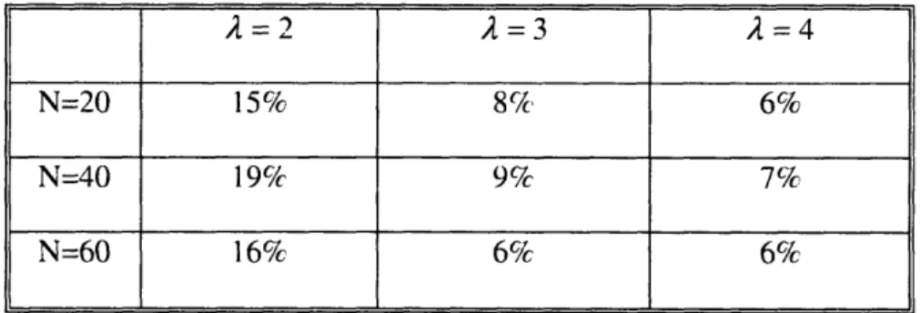
Table 2-3 shows the average power saving ratio of the broadcast trees generated by RTO compared with BIP for the same network topologies with different number of nodes and different power attenuation factor values. Clearly, the RTO algorithm outperforms BIP across the all setups. In comparison with Table 1, we observe that RTO performs better than combining BIP with IMBM. The advantage of RTO over BIP with IMBM is most noticeable

for A equals 2, where the average power saving is around 10%.

Table 2-3: Average power saving ratio of the normalized tree power of the broadcast trees generated by RTO compared with BIP (50 randomly-generated network instances for each group).

A=2

N=20 15% 8% 6%

N=40 19% 9% 7%

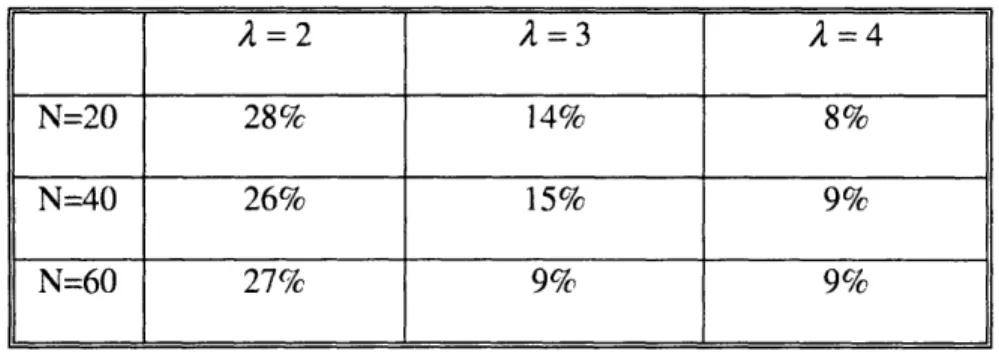
Table 2-4 demonstrates the average power saving ratio of the broadcast trees generated by RTO compared with MST for the same network topologies for three values of A. In comparison with Table 2-2, we can clearly see that RTO performs better than MST+IMBM, in particular when A equals 2, the average power saving is around 20%.

Table 2-4: Average power saving ratio of the normalized tree power of the broadcast trees generated by RTO compared with MST (50 randomly-generated network instances for each group).

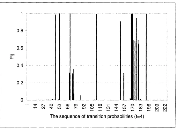
In order to provide some more insight into the inner working of the RTO algorithm, we show the evolution of the transition probability matrix for a single run of the RTO algorithm in Figure 2-1. We randomly generated N= 15 nodes, and set A to 2. The initial sequence of the

q, s is based on Equation (4). with c set to zero.

In the Figure 2-1, we plot a histogram of all the q,. s for different iterations. The y-axis denotes the one-step transition probability. The x-axis stands for the sequence of the elements in the probability matrix and we have a total of 15X 15 = 225 (N=15) elements in the matrix.

A=2 2=3 A=4

N=20 28% 14% 8%

N=40 26% 15% 9%

As typical to the CE method, the transition probabilities quickly converges with some

transition probabilities converging to one and others to zero. Essentially, transitions that lead to good solutions are reinforced and transitions that lead to poor solutions become smaller.

1 0.9 0.8 0.7 06 5~' 0. 4053

0.2

nJ t al sequence f tn - i pra i1e (t

=0)-Initial sequence of transition probabilities (t=0)

1 0.9 0.8 0.7 0.6 i 0.5 0.4 0.3 0.2

0.1

1 0.9 0.8 0.7 0.6 I~' O.5 0.4 0.3 0.2 0.1 0 - -- - - -L .. L i S -NO (0 0) C LO CO 1- O o N C I LO QOO r- It LM M N

The sequence of transition probabilities (t=2)

1 -0.9 0.8 0.7 0.6 80.5 0.4 0.3 0.2 0.1

0.8 0.6 0.4 0.2 0 - e- 0C M Co c MW Io '- N. o ' N ' LM Co N- ) C'q M LO ) N

The sequence of transition probabilities (t=4)

Figure 2-1: An illustration of an example run of the evolving of the transition probability matrix (N =15, A =2) during the RTO process.

In order to demonstrate the robustness of the RTO algorithm to its parameters, we varied the smoothing parameter a.

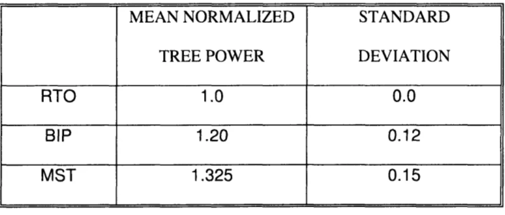
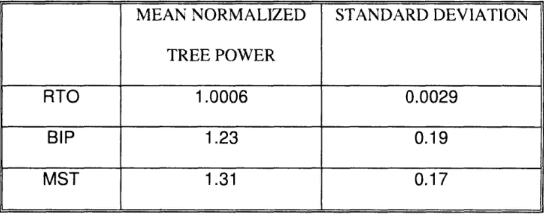
In Table 2-5 and Table 2-6 we provide the normalized tree powers by RTO, BIP and MST for 30 randomly-generated network instances with different values of the transition probability update smoothing factor a .

The number of nodes in the network, i.e., N , is 15, and the value of A is 2. For the results reported in Table 2-5, the value of a is 0.8. For the results reported in Table 2-6, the value of a is 0.7. In Table 2-5, the average normalized tree power for RTO, BIP and MST are 1.0, 1.20 and 1.325, respectively. The standard deviation for RTO, BIP and MST are 0.0, 0.12 and 0.15, respectively. In Table 2-6, the average normalized tree power for RTO, BIP and MST are 1.0006, 1.23 and 1.31, respectively.

It can be observed that RTO outperforms the other two algorithm in terms of both average performance and low standard deviation. In the following experiments, we use the value of 0.8 for a unless explicitly specified otherwise. By examining the values in Table 2-5 and Table 2-6, we observe that RTO significantly outperforms BIP and MST for N is 15 and A is 2. In some cases, RTO saves as much as 60% to 90% power compared with BIP and MST.

Table 2-5: Normalized tree power by RTO, BIP and MST for 30 randomly generated networks. The number of nodes in the network, i.e., N, is 15, the value of A is 2 and the

value of a is 0.8.

MEAN NORMALIZED STANDARD

TREE POWER DEVIATION

RTO 1.0 0.0

BIP 1.20 0.12

MEAN NORMALIZED STANDARD DEVIATION TREE POWER

RTO 1.0006 0.0029

BIP 1.23 0.19

MST 1.31 0.17

Table 2-6: Normalized tree power by RTO, BIP and MST for 30 randomly generated networks. The number of nodes in the network, i.e., N , is 15, the value of A is 2 and the value of a is 0.7.

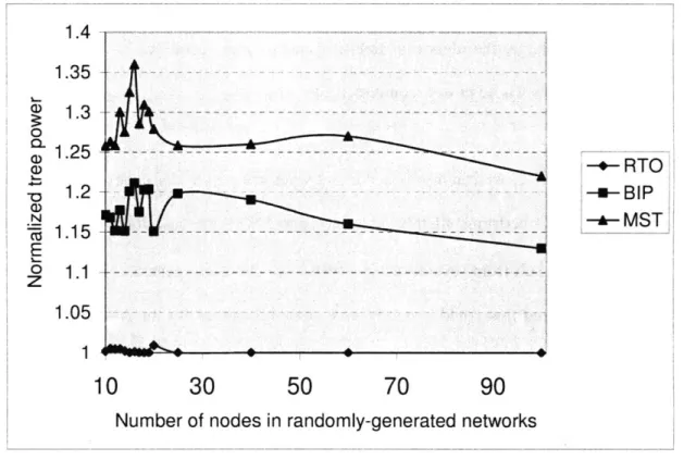
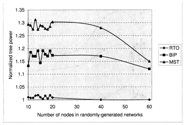
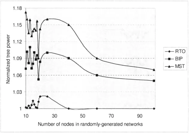
We now consider the other parameter of the RTO method - the initialization procedure. In Figure 2-2 and Figure 2-3 we present the average normalized tree power by RTO, BIP and MST with different initialization methods of the transition probability matrix when the value of A is 2.

For the results in Figure 2-2, we initialize the probability matrix according to Equation (4), when N is less than 40, we choose c as zero; when N is between 40 and 60, we choose c as half of the diameter of the network; when N is greater than 60 se choose c as the diameter of the network. For the results in Figure 2-3, the initial transition matrix is set with equal

probability of for each qj1 (this is equivalent to choosing a large c).

The number of nodes in the network ranges from 10 to 100 in Figure 2-2 and the number of nodes ranges from 10 to 60 in Figure 2-3. Notably, for a small value of N , say N is less than 40, both initialization methods lead to good performance of RTO, while for a large value of N, the performance of the equal probability initialization method degrades, as shown in Figure 2-3. We attribute this to the fact that equal probability initialization method does not reflect the power requirement for each transition. Consequently, when the number of nodes is large, the algorithm fails to generate any "good" trees to start with and only generates trees whose power requirements are large.

From Figure 2-2, we can also observe that when the number of nodes in the network is less than 20, RTO performs slightly better compared with the case for a larger number of N. This could result from several factors: firstly, we choose to generate 20N 2 _{sample trees for}

each round and this could certainly give some advantage for an N smaller than 20. If we choose to generate N3 _{sample trees, we expect that the curve could be flat but the algorithm}

would be slower. Secondly, we use a loose termination criterion for a large N to speed up the RTO process and this could also cost some performance gains.

Figure 2-4 and Figure 2-5 show the results of the normalized tree power by RTO, BIP and MST for the same network topologies with different number of nodes when the value of A is 3 and 4 respectively. Clearly, the power savings by RTO compared with BIP and MST degrades with a larger value of A. This trend is consistent with the results of EWMA compared with BIP and MST reported in [1]. As A becomes large, the advantage of using the RTO method degrades since incremental approaches like BIP and MST performs reasonably

well for a fast power attenuation environment. For example, for a very large value of A, the best trees would connect every node to its closest neighbor (since any transmission beyond the minimal possible is prohibitive). Since our performance measure is the ratio between performances, the advantage of the RTO becomes less significant for large values of A.

1.4 1.35 ( 1.3 0 CD 1.25 - 1.2 a> N a 1.15 E 1.05 1 -+-RTO -u- BIP -*-MST

10

30

50

70

90

Number of nodes in randomly-generated networks

Figure 2-2: Average normalized tree power by RTO, BIP and MST (average over 60 randomly generated network instances for networks with a fixed number of nodes) with different number of nodes in the network and adaptive transition probability matrix initialization for RTO. The value of A is 2.

1.35 1.3 1.25 1.2 1.15 1.1 1.05 1 -+- RTO -u-BIP -*- MST - -- - - - - - - - - - - - - - - -- - - - ---- -

--

--

_{--- ---}

Number of nodes in randomly-generated networks

Figure 2-3: Average normalized tree power by RTO, BIP and MST (average over 60 randomly generated network instances for networks with a fixed number of nodes) with different number of nodes in the network and equal-probability initialization of the transition probability matrix for RTO. The value of A is 2.

1.18 1.15 1.12 0 +-R TO - 1.09 -- -- -- -- - - - B IP N-a- MST 1.06- -- - - - - - ---- - --- -0 1.03 1 10 30 50 70 90

Number of nodes in randomly-generated networks

Figure 2-4: Average normalized tree power by RTO, BIP and MST (average over 60 randomly generated network instances for networks with a fixed number of nodes) with different number of nodes in the network. The initial transition matrix is set according to Equation (4). The value of A is 3.

- RTO

-U- BIP

MST

10 30 50 70 90

Number of nodes in random ly-generated networks

Figure 2-5: Average normalized tree power by RTO, BIP and randomly generated network instances for networks with a fixed different number of nodes in the network. The value of A is 4.

MST (average over 60 number of nodes) with

Notably, in this chapter we assume that only one transmitting node is engaged in a one-to-one or one-to-one-to-many transmission. In the next chapter, we will explore transmit diversity in the general context of cooperative routing, whereby multiple nodes are allowed for cooperative transmissions. The techniques presented in the next chapter can be further incorporated in the approaches for the construction of cooperative multicast trees proposed in this chapter.

1.12

1.09

1.06

Chapter 3

Cooperative Routing in Wireless Networks

3.1

The Overview

As mentioned at the end of Chapter 2, in this chapter we explore transmit diversity in the general context of cooperative routing where multiple nodes are allowed for cooperative transmissions. In Chapter 2, we assume that only one transmitting node is engaged in a one-to-one or one-to-many transmission. The techniques presented in this chapter can be further incorporated in the approaches for the construction of cooperative multicast trees presented in Chapter 2. Cooperative routing approach allows multiple nodes along the path for cooperative transmission (transmit diversity) to the next hop so long as the combined signal at the receiver satisfies the threshold value of SNR (signal-to-noise ratio). We say a transmission is successful only if the SNR of the received signal at the receiver is above a given threshold value, say SNRmin . The threshold value of SNRmin is chosen to achieve a desired BER (bit error rate) for the given modulation scheme and data rate [28]. Traditional routing scheme solely assumes the role of route selection based on some criteria such as the number of hops on the path, the cost of the path and/or some QoS parameters, while the cooperative routing approach combines route selection and the exploration of transmit diversity and the resulted cross-layer design method may be beneficial in wireless networks.

The motivation of this work is two-fold. The first is the importance of energy efficiency in wireless networks. The lifetime of a wireless network is limited due to the limited power

capacity of the energy sources at each node such as batteries. The lifetime of such a wireless network totally depends on the energy consumption of each node. To increase the longevity of such networks, power-efficient and power-aware protocols and techniques including link layer, MAC, routing and transport protocols must be employed to minimize the power consumption (we will use energy and power interchangeably throughout the thesis). As will be seen later in this chapter, the cooperative shortest path algorithm can save about 30-50% power compared with non-cooperative shortest path algorithm, depending on the node density of the network. The empirical results indicate that as more nodes added in the network, more power savings compared with non-cooperative scheme can be achieved by the presented approach in that a dense network offers more opportunities for cooperative transmission.

The second motivation is for the scalability of the network. Wireless networks face scalability problems, in particular in large and dense networks, as transmitting with excessive power on one link often leads to severe interference to other links in the system. As discussed in [28], a wireless link is rather a "soft" concept in the sense that a "link" exists between two wireless nodes if the transmitting node transmits with sufficiently high power such that the SNR at the receiving node is above a given threshold, say SNRr,111. Moreover,

wireless channel inherently has fundamental impairments due to multi-path fading, attenuation, reflection, obstruction, etc., besides interference and noise. As such, our objective is to optimize the distribution of information by exploring transmit diversity and to minimize the wireless channel impairment effects via cooperation among nodes in the network such that the network scales well. Further, optimizing the transmissions to achieve

more fairness among nodes also makes the network more scalable in that fairness in resource allocation often leads to maximized transmission capacity. The concept of fairness here means the distribution of information in the network is optimized in such a way that each node is treated fairly based on the pre-defined utility function for each node (we will have more discussion on this in Section 3.6). As we will see later in the thesis that the cooperative routing approach substantially reduces the total consumed power along the path compared with the non-cooperative counterpart. Hence, the presented approach leads to less interference among transmitting nodes with considerably reduced transmitting power. Moreover, the experimental results also suggest that as more nodes added in the network, our approach achieves more fairness while the fairness curve for other existing schemes are mostly flat (see Fig. 3-6 for details).

The minimum energy cooperative path routing problem in wireless networks has been recently addressed in 113] and several heuristic algorithms were developed to approximate the minimum energy route based on non-cooperative shortest-path algorithm. One of the presented algorithms in 113] is called CAN (cooperative along non-cooperative shortest path). The basic idea is to run a non-cooperative shortest path algorithm to obtain the cooperative path. The computational complexity of CAN algorithm is in the order of O(N 2_),

where N is the number of nodes in the network. Let L denote the number of nodes that are allowed for cooperative transmission along the path, and following [13] we always assume that the last L nodes along the path for cooperative transmission to the next hop. Another heuristic algorithm presented in [131 is called Progressive Cooperation (PC) algorithm. The PC algorithm operates progressively by iteratively calculating the non-cooperative shortest

path from the Super node (initialized as the source node only) to the destination node based on updated link cost and combining the last L nodes along the current best path as one single Super node until the destination is included. Our presented cooperative shortest path algorithm (CSP) operates differently with the PC algorithm in that the CSP algorithm proceeds as a cooperative version of Dijkstra's algorithm with a new relaxation procedure to reflect the cooperative transmission cost and every time one un-included node with the least cooperative transmission cost along the current best path from the source node is added to the list who already find the cooperative shortest path from the source node instead of calculating the whole non-cooperative shortest path to include (L -1) new nodes at one time. The resulted CSP algorithm has the complexity of O(N2_{), while the complexity of the PC} algorithm is in the order of O(N 3_).

Our work builds upon that of Khandani et al 113]. In this thesis, we first prove that the minimum energy cooperative path (MECP) problem is NP-complete. We then propose a cooperative shortest path algorithm (CSP) that uses Dijkstra's algorithm as the basic building block and reflects the cooperative transmission properties in the relaxation procedure. Our approach consistently outperforms the heuristics in 1131 in terms of energy consumption for the same settings with the same computational complexity of O(N ) as that of CAN algorithm (again, N is the number of nodes in the network). Another interesting finding is that the presented approach achieves more fairness as more nodes added in the network. which reflects the fact that the cooperative shortest path algorithm adapts itself more efficiently to the cooperative routing settings and better exploits the cooperative opportunities among nodes in the network.

Another closely related work by Catovic et al in 12] referred the concept of cooperative routing as power combining .They present approaches to explore transmit diversity via user cooperation in next generation wireless multi-hop networks. The network model used in

121 greatly differs from that assumed in [13]. We will discuss the detailed network model and assumptions in Section 2. In essence, Catovic et al assume that the m-finger RAKE receivers are used for wideband communications and each finger is in charge of the reception of the signal from a different transmitter. Khandani et al in [131 consider that conventional receivers are used and the channel parameters are estimated by the receiver and fed back to the transmitter. It is essentially a tradeoff between the use of complex receivers, e.g., the m-finger RAKE receivers, and the complexity to implement the feedback mechanism. The bottom line is that the feedback-based model in 113] can achieve more energy savings due to the coherent combining of the signals from multiple transmitters. Nevertheless, the basic

framework of the algorithm presented in this thesis can be equally applicable to other cooperative routing environment, e.g., different fading/attenuation models, different receiver

types, etc.

Other researchers also address the power efficiency issue in wireless networks. Wieselthier et al [32], Calgalij et al I I] and Liang [19] presented approaches for the construction of minimum energy broadcast trees in wireless networks. In particular, the seminal work by Wieselthier et al in 1321 elucidates many fundamental aspects of energy-efficient routing in wireless networks. Rodoplu and Meng 1261 proposed a novel distributed position-based network protocol to achieve the minimum-energy network topology. Wattenhofer et al [31]

presented an ingenious distributed topology control algorithm for power efficiency in wireless ad-hoc networks based on directional information.

Min and Chandrakasan address the energy consumption issues of wireless communication in [22]. In [9], Feeney and Nilson reveal that nodes usually spend most of their energy in communication in wireless ad hoc networks. Srinivas and Modiano [28] presented algorithms for finding minimum energy disjoint paths in wireless ad hoc networks for the sake of energy efficiency and reliability. The work in 128] elucidates many of the network model concepts that are used in this work.

The major contribution of this thesis is the proof of the NP-completeness of the minimum energy cooperative path (MECP) problem, the development of a cooperative shortest path (CSP) algorithm for cooperative routing in wireless networks and the exploration of the impact of the presented approach on energy savings, fairness and network scalability compared with existing approaches.

The rest of this chapter is organized as follows. We give the description of the system model in Section 3.2 and the problem formulation in Section 3.3. We prove the NP-completeness of the minimum energy path problem in the context of cooperative routing in Section 3.4 and we present a cooperative shortest path algorithm for cooperative routing in Section 3.5. The experimental results, which are presented in Section 3.6, demonstrate the high performance of our algorithm compared with other cooperative routing algorithm and non-cooperative shortest path algorithms. Distribution and implementation issues are discussed in Section 3.7.