Problems in Mathematical Analysis pdf - Web Education

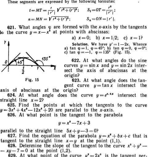
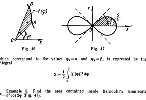
TEXT

FLY

WITHIN

OU_1

58871

>

OUP-43

30-1.71 5,000

OSMANIA

UNIVERSITY

_LIBRARY

Call No.

_g>^^

Accession No.

Author

M

I

R

T. C. BapaneHKoe. B. 77 AeMudoeuH, B.

A

C.

M.

Koean,

r

Jl JJyHit,

E

noptuneea,

E

H. Ctweea,

C. B. <Ppo/io8> P. fl. UlocmaK, A. P.

SAflAMM H

VnPA)KHEHHfl

no

MATEMATM

H

ECKOMV

AHAJ1H3V

I7od B. H.

AE

rocydapcmeeHHoe a

M

G.

Baranenkov*

B.

Drmidovich

V.

_Efimenko,

S.

_Kogan,

G.

Lunts>>

E.

Porshncva,

E.

bychfia,

S. frolov, /?. bhostak,

A.

_Yanpolsky

PROBLEMS

IN

MATHEMATICAL

ANALYSIS

Under the editorship of

B.

DEMIDOVICH

Translated from the Russian

by G.

YANKOVSKV

MIR PUBLISHERS

TO

THE READER

MIR

Publishers would be _glad to have _your

opinion of the translation and the design of this

book.

Please send your suggestions to 2, _{Pervy Rtzhtky}

Pereulok, Moscow, U. S. S. R.

Second _Printing

CONTENTS

Preface 9

Chapter I.

INTRODUCTION

TO

ANALYSIS

Sec. 1. Functions 11

Sec. 2 Graphs of _Elementary Functions 16

Sec. 3 Limits 22

Sec. 4 Infinitely Small and Large Quantities 33

Sec. 5. _Continuity of Functions 36

Chapter II

DIFFERENTIATION OF FUNCTIONS

Sec 1. _Calculating Derivatives _Directly 42

Sec 2 Tabular Differentiation 46

Sec. 3 The Derivatwes of Functions _{Not Represented Explicitly} . . 56

Sec. 4. Geometrical and Mechanical _Applications of the Derivative . 60

Sec 5 Derivatives of _{Higier Orders} 66

Sec 6 Differentials of First and Higher Orders 71

Sec 7 Mean Value Theorems 75

Sec. 8 _Taylor's Formula 77

Sec 9 The _{L'Hospital-Bernoulli} Rule for Evaluating Indeterminate

Forms 78

Chapter III

THE

EXTREMA

OF A

FUNCTION

AND

THE GEOMETRIC

APPLICATIONS OF

A

DERIVATIVE

Sec. 1. The Extrema of a Function of One _Argument 83

Sec. 2 The Direction of _Concavity Points of Inflection 91

Sec 3 _Asymptotes . 93

Sec 4. _Graphing Functions by Characteristic Points 96

Sec. 5. Differential of an Arc Curvature . . 101

Chapter IV

INDEFINITE

INTEGRALS

Sec. 1 Direct _Integration 107

Sec 2 Integration by Substitution 113

Sec 3 _Integration by Parts 116

Sec. 4 Standard _Integrals Containing a _{Quadratic Trinomial}

....

118

Contents

Sec. 6. Integrating Certain Irrational Functions 125 Sec 7. _{Integrating Trigoncrretric} Functions 128 Sec. 8 Integration of Hyperbolic Functions 133

Sec 9. _{Using Ingonometric and} Hyperbolic Substitutions for _Finding

integrals of the Form f

R

(x,

^a^

+

bx

+

c)dx, Where

R

is a

Ra-tional Function 133

Sec 10 Integration of Vanou* Transcendental Functions 135

Sec 11 Using Reduction Formulas 135

Sec. 12. Miscellaneous _Examples on _Integration 136

Chapter V

DEFINITE

INTEGRALS

Sec. 1. The Definite Integral as the Limit of a

Sum

138

Sec 2 Evaluating Ccfirite Integrals by Means of Indefinite Integrals 140

Sec. 3 Improper Integrals 143

Sec 4 _Charge of Variable in a Definite _Integral 146

Sec. 5. _{Integration by} Parts 149

Sec 6 Mean-Value Theorem 150

Sec. 7. TheAreas of Plane _Figures 153

Sec 8. The Arc Length of a Curve 158

Sec 9 Volumes of Solids 161

Sec 10 The Area of a Surface of Revolution 166

Sec 11 torrents Centres of _Gravity Guldin's Theorems 168

Sec 12. _{Applying Definite Integrals}to the Solution of _Physical

Prob-lems 173

Chapter VI.

FUNCTIONS OF

SEVERAL VARIABLES

Sec. 1. Basic Notions 180

Sec. 2. _Continuity 184

Sec 3 Partial Derivatives 185

Sec 4 Total Differential of a Function 187 Sec 5 Differentiation of _Composite Functions 190

Sec. 6. Derivative inaGiven Directionand the Gradient of a Function 193

Sec. 7 HigKei-Order Derivatives and Differentials 197

Sec 8 Integration of Total Differentials 202 Sec 9 Differentiation of _Implicit Functions 205

Sec 10 _Change of Variables .211

Sec. 11. _{The Tangent Plane and} the Normal to aSurface 217

Sec 12 _Taylor's Formula for a Function of Several Variables . . . 220

Sec. 13 The Extremum of a Function of Several Variables

....

222

Sec 14 Firdirg the Greatest and *tallest Values of Functions . . 227

Sec 15 Smcular Points of Plane Curves 230

Sec 16 _Envelope . . 232

Contents

Sec. 18. The Vector Functionof a Scalar _Argument 235

Sec. 19 The Natural Trihedron of a _Space Curve 238

Sec. 20. Curvature and Torsion of a _Space Curve 242

Chapter VII.

MULTIPLE

AND

LINE

INTEGRALS

Sec. 1 The Double _Integral in Rectangular Coordinates 246

Sec. 2 Change of Variables in a Double Integral 252

Sec. 3. _Computing Areas 256

Sec. 4. _{Computing Volumes} 258

Sec. 5. _Computing the Areas of Surfaces 259

Sec. 6 _Applications of the Double Integral in Mechanics 230

Sec. 7. Triple Integrals 262

Sec. 8. _Improper Integrals Dependent on a Parameter. _Improper

Multifle Integrals 269

Sec. 9 Line Integrals 273

Sec. 10. Surface _Integrals 284

Sec. 11. The_{Ostrogradsky-Gauss}Formula 286

Sec. 12. Fundamentals of Field _Theory 288

Chapter VIII. SERIES

Sec. 1. Number Series 293

Sec. 2. Functional Series 304

Sec. 3. _{Taylor's Series} 311

Sec. 4. Fourier's Series 318

Chapter

IX

DIFFERENTIAL EQUATIONS

Sec. 1. _{Verifying Solutions.} Forming Differential _Equations of

Fami-lies of Curves. Initial Conditions 322

Sec. 2 First-Order Differential _Equations 324

Sec. 3. First-Order Diflerential _{Equations with Variables Separable.}

Orthogonal Trajectories 327

Sec. 4 First-Order Homogeneous Differential Equations 330

Sec. 5. First-Order Linear Differential _Equations. Bernoulli's

Equation 332

Sec. 6 Exact Differential Equations. Integrating Factor 335

Sec 7 First-Order Differential EquationsnotSolvedfor the Derivative 337

Sec. 8. The _Lagrange and Clairaut _Equations 339

Sec. 9. Miscellaneous Exercises on First-Order Differential _{Equations 340}

Sec. 10. Higher-Order Differential _Equations 345

Sec. 11. Linear Differential _Equations 349

Sec. 12. LinearDifferential_Equations of Second Order with Constant

8 Contents

Sec. 13. Linear Differential _Equations of Order _Higher than

Two

with Constant Coefficients 356

Sec 14. Euler's_Equations 357

Sec 15. _Systems of Differential _Equations 359

Sec. 16. _Integration of Differential _{Equations by} Means of Power

Se-ries 361

Sec 17. Problems on Fourier's Method 363

Chapter X.

APPROXIMATE CALCULATIONS

Sec. 1 _{Operations on Approximate} Numbers 367

Sec. 2. _{Interpolation} of Functions 372

Sec. 3. _Computing the^Rcal Roots of _Equations 376

Sec. 4 Numerical, Integration of Functions 382

Sec. 5. Nuner:ca1 Integration of _Ordinary DilUrtntial _Equations . . 384

Sec. 6. _{Approximating Ftuncr's} Coefficients 3>3

ANSWERS

396

APPENDIX

475

I. Greek Alphabet 475

II. Some Constants 475

III. Inverse Quantities, Powers, Roots, Logarithms 476

IV Trigonometric Functions 478

V. Exponential, Hyperbolic and Trigonometric Functions 479

PREFACE

This collection of _problems

and

exercises in mathematical

anal-ysis covers the

maximum

requirements of general courses in

higher

mathematics

for _higher technical schools. It contains over

3,000 problems sequentially arranged in _Chapters I to

X

_covering

all branches of _higher

mathematics

_(with the _exception of

ana-lytical geometry) given in _{college courses.} Particular attention is

given to the most _important sections of the course that _require

established skills (the finding of limits, differentiation _techniques,

the _graphing of _{functions, integration techniques, the applications}

of definite _integrals, series, the solution of differential equations).

Since

some

institutes have extended courses of _mathematics,

the authors have included _problems

on

field _theory, the Fourier

method, and

_approximate

calculaiions. _Experience

shows

that the

number

of _{problemsgiven} in this book not _{only fully} satisfies

the _requireiren s of the student, as far as _{practical mas!ering} of

the various sections of the course goes, but also enables the

in-structor to _supply a varied choice of

_problems

in each section

and

to select _problems for tests and examinations.

Each

chap.er begins with a brief theoretical introduction that

covers the basic definitions

and

formulas of that section of the

course.

Here

the most _{important typical problems} are

worked

out

in full.

We

believe that this will _{greatly simplify} the

work

of

the student.

Answers

are _given to all _{computational problems;}

one asterisk indicates that hints to the solution are given in

the answers,

two

asterisks, that the solution is _given.

The

problems

are _frequently illustrated _{by drawings.}

This collection of _problems is the result of

_many

_years of

teaching higher

mathematics

in the technical schools of the Soviet

Union. It _includes, in addition to _{original problems}

and

Chapter I

INTRODUCTION TO

ANALYSIS

Sec. 1. Functions

1. Real nurrbers. Rationalandirrational numbers are collectively known

as real numbers The absolute value of a real number a is understood to be

the nonnegative number \a\ defined by the conditions'

_\a\=a

if

a^O,

and

|aj

=

a if a

<

0. The following inequality holds for all real numbers a

ana b:

2. Definition of a function. If to _{every value*)} of a variable x, which

belongs to son.e collection (set) E, there _{corresponds one and only one} finite

value of the quantity /, then y is said to be a _function (single-valued) of x

or a _dependent tariable defined on the set E. x is the ar

gument or

indepen-dent variable The fact that y is a Junction of x is _expressed in brief form

by the notation _y~l(x) or _y

=

F(A), and the 1'ke

If to every value of _{x belonging} to some set E there _corresponds one or

several values of the variable /y, then y is called a multiple-valued function of x defined on E. From now on we shall use the word "function" only in

the meaning of a single-valued function, if not otherwise stated

3 The domain of definition of afunction. The collectionof valuesofxfor

which the given function is defined is called the domain of definition (or the

domain) of this function. In _{the simplest} cases, the domain of a function is

either a closed interval [a.b\, which is the set of real numbers x that satisfy the inequalities

a^^^b,

or an open intenal (a.b), which :s the set of real

numbers that_{satisfy the inequalities a}

<

x

<

b. Also possible is a more

com-plex structure of thedomainof definition of afunction (see, for instance,

Prob-lem 21)

Example 1. Determine the domain of definition of the function

1

Solution. The function is defined if

x2

-l>0,

that is, if

_|x|>

1. Thus, the domain of the function is a set of two inter-vals:

oo<x<

1 and 1

<

x

<

-\-oo

4. Inverse functions. If theequationt/

=

/(x) may be solved uniquely for

the variable x, that is, if there is a function x _{g(y) such} that _y^*

*) Hencetorth all values will be considered as real, if not otherwise

12 Introduction to Analysis \Ch. I

then the function x

=

g(y), or, in standard notation, y=g(x), is the inverse of _y

=

_f(x). Obviously, g[f(x)]s&x, that is, the function f (x) is the inverse

of _{g(x) (and} vice ve^sa).

In

He

fereia! case, the equation y f(x) defines a _{multiple-valued}

in-verse function x

=

f~}

(y) such that y==[[(-*(y)\ for all y that are values of

the function f (x)

Lxanple 2. Determine the inverse of the function

y=l-2-*.

(1)

Solution. Solving equation (1) for x, we have

2-*=l

y and log(l-y) * log 2 j'

w

Obviously, the domain of

Definition of the function (2) is oo

</<!.

5. Corrposite and irrplicit functicns.

A

function y of x defined by a se-ries of _equalitiesy

=

_{/(), where}u

=

₉(x), etc., is called a comoosite function, or a _function of a function.

A function defined by an equation not solved for the dependent variable

is called an implicit (unction. For example, the equation x*+i/*=l defines

y as an implicit function of x.

6. The graph of a function.

A

set of _points (x,y) in an _;o/-plane, whose

coordinates are connected _by the equation y f(x), is called the _graph of

the given function.

1**. Prove that if a

and

b are real

numbers

then

\\a\-\b\\<\a-b\<\a\

+

\b\. 2. Prove the _{following equalities:}

a)

|ab|Ha|.|b|;

c) b) |a|

2

=

a2

; d)

3. Solve the inequalities:

a) |x

1|<3;

c) * b)

|x+l|>2;

d) |jt-4. _{Find /(-1),/(0),/(1), /(2), /(3), /(4),} if _/(*)

=

*'-

6*' -f 4- llx 6. 5. Find _/(O),

/(-4).

/(-^/(T)

7^.

if/

6. /(x)

-arc

cos(logx). Find

/!,

/(I), /(10).

7.

The

_{function f(x)} is linear.

Find

this _{function, if/( 1)}

=

2

and

_/(2)

=

3.

Sec 1] Functions 13

8. Find the rational integral function f(x) of degree two, if

=

and /(3)

=

5.

9.

Given

that f(4)

=

2, /(5)

=

6.

_Approximate

the value of

/(4, 3) if

we

consider the function / (x)

on

the interval

linear _{(linear interpolation of} a _function).

10. Write the function

0, if

as _{a single} formula using the absolute-value sign.

Determine

the

domains

oi definition of _{the following functions:}

11. _{a) y}

=

_x+\;

16.

_y

=

x

-17. /

=

lo 13.

_a),=

_?E2L

b) (/

=

*VV-2.

19. t/= 14**.

=1/2

+

*

**.

-21. Determine the

domain

of definition of the function

y

=

|/sin2x.

22. _f(jc)

=

2A:4 SA;' 5x8

₊

6A: 10. Find

(-*)l

and ^(^)

=

23.

A

function _f(x) defined in a

_symmetric

_region /

is called euen if _{f( x)}

=

_f(x) and orfd if _{/( x)}

=

f(x).

Determine

which

of _{the following functions} are even

and which

are odd:

e)

24.

Prove

that

_any

function _f(x) defined in the interval

/<;*</

may

be _represented in the form of the

sum

of an

14 Introduction to Analysis [Ch. 1

25. Provethat the product of

two

even functions or of

two

odd

functions is an even function, and that the _product of an even

function _by an

odd

function is an

odd

function.

26.

A

function f(x) is called _periodic if there exists a _positive

numter

T

(the period of the function) such that

f(x+ T)^f(x)

for all valves of x within the

dcmain

of definition of _f(x).

Determine

uhich

of the following functions are _periodic,

and

for the _periodic functions find their least _period T:

a) / (x)

=

10 sin3*, d) /(x)

=

sin

1

*;

b) /(*)

=

a sin\K

+

b costar; e) / (x)

=

sin (J/*).

c)

27. _Express the _length of the _{segment y}

=

MN

and the area

S

of the _figure

AMN

as a function of

x=AM

_(Fig

1). Construct

the _graphs of these functions.

28.

The

linear _{density (that} is,

mass

_{per unit length)} of a rod

AB

=

l

(Fig. 2) on the segments

AC

l^

CD

=

1

2 and

DB =

l\ (/t

+

lt + /3

=-1)

AfsM"

M

\ I f is equal to </,, qz

and

q^

respec-B

B

Fig. 1 _Fig. 2

tively. Express the

mass

m

of a variable _segment

AM =

x

of this

rod as a function of x. Construct the _graph of this function.

29. Find cp|\M*)|

and

i|?jtp(x)J, if _v(x)

=

x?

and

_q(x)

=

2*.

30. Find

_H/Um,

if

31. Find

_/U+l),

if _{f(x l)}

=

x\

32. Let _{f(n) be the}

sum

of n terms of an _{arithmetic progression.}

Show

that

33.

Show

that if

f(x)

=

and

the

numbers

jc

lf

x

t,

x

_t form an arithmetic _progression, then

the

numbers

_J(xl)9 f(xt)

and

/(xj likewise form such a

Sec. 1]

_

Functions

_

15

34.

Prove

that if _f(x) is an _{exponential function,} that is,

/ (x)

=

a

x

(a

>0),

and the

numbers

x

v

*,, xt form an arithmetic

progression, then the

numbers

/(*,), f(*2 ) and /(jcj form a

geo-metric _progression.

35. Let

Show

that

36. Let <p(*)

=

!(*

+

a-*)

and

t|)(AT)

= 1

(a* a-*).

Show

that

f

p(*+</)

=

<p

W

<p(y)

+

*

(*)^>(y)

and

ty(x

+

y) <p

37.

_{Find /(-I),}

_{/(O), /(I)} if

arc sin

x

for 1

^

r

^

0,

arctanxfor

<

# c

+

oo.

38.

Determine

the roots _(zeros) of_{the rrgion} of _positivity

and

of _{the region} of _negativity of the function _y if:

a) r/=l -f-x; d)

y

=

x* 3x;

b) y

=

2

+

x *2;

^

ff

_

ioo 2jc

c)

0=1

-39. Find the inverse of the function _y if:

In

what

_regions will these inverse functions be defined?

40.

Find

the inverse of the function

/ x, if

y

\ x*, if

41. Write the _given functions as a series of _equalities each

member

of

which

contains a _{simple elementary} function _(poweri

exponential, trigonometric, and the like):

a) i/

=

(2*-5r;

_c)

_y

b) y

=

2COS*; _d)

y

=

arc sin_(3-*

3 ).

16 Introduction to Analysts [Ch. 1

42.

Write

as a _{single equation} the _composite functions

repre-sented as a series _{of equalities:}

a) y

=

u*> w

=

sin#;

b) #

=

arctan,

u

=

Yv,

y

=

_log#;

w, if

_t/<0,

,

ifu>0;

*_!.

43. Write, explicitly, functions of

y

defined

_by

_{the equations:}

a)

x

2

arccos _y

=

n;

b) 10*

+10'

=10;

c)

*

+

\y\

=

2y.

Find the

domains

of definition of _{the given implicit} functions.

Sec, 2. _Graphs of _Elementary Functions

Graphs of _{functions #}

=

/(*) are _mainly constructed _{by marking} a

suffi-ciently dense net of points Ai/(*,-, //), where */,

=

/(*,-)(/

=

0, 1, 2, ...) and

byconnectingthe pointswith a line that takes account of intermediate points.

Calculations are best done by a slide rule.

Fig. 3

Graphs of the basic elementary functions _(see

_Ap

_{pendix VI)} are _readily

learned through their construction. _Proceeding from the graph of

y

=

f(x), (T)

we get the graphs of the following functions _by means of simple geometric

constructions:

1) 0i

=

M*) _js th* mirror image of the graph T about the *-axis;

Sec. 2] Graphs of Elementary functions 17

3) #i

=

/(*)

is the F graph displaced along th? x-axis _{by an} amount a;

4) 1/4

=

&

+

/(*) is the F graph displaced along Uve (/-axis by an amount

(Fg. 3).

Example. Construct the graph of the function

Solution. The desired line is a sine curve y

=

sinx displaced along the *-axis to _{the right by} an amount

-j (Fig. 4)

Y

Fig. 4

Construct the _graphs of the _following linear functions

(straight lines):

44. _y

=

_kx, if fc

=

0, 1, 2, 1/2,

-1, -2.

45. i/

=

x+

6, if 6

=

0, 1, 2, 1, 2.

46.

_0=1.

5*

+2.

Construct the _graphs of rational _integral functions of _degree

two

(parabolas). 47. _y=--ax3, if

a=l,

2, 1/2, 1, 2, 0. 48. _//

=

*'-{-c, if

c=0,

_{1, 2,} 1. 49.

_,/=(*-*)',

if *.

=

f 1, 2,

-1.

50. _y

=

_y, 4

_(x-l)\

if </

=

0, 1, 2,

-1.

51*.

_y

=

ax*

+

bx

₊

c, if: ₁₎

a=l,

b

=

2, c

=

3; 2) a

=

2,

6

=

6, c

=

0.

52. t/

=

2 f

x

x*.

Find

the points ol intersection of this

pa-rabola with the Ac-axis.

Construct the _graphs of the _{following rational integral}

func-tions of _degree

above

two:

53*.

_y

=

x* _{(cubic parabola).}

54. </

=

2

+(*-!)'.

55. _t/

=

x' _3x-\-2.

56.

_y

=

x\

57.

y

=

2x'-x*.

Construct the _graphs of the _following linear fractional

func-tions _{(hyperbolas):}

18

_

Introduction to Analysis

_

[Ch. 1

59.

-.

61*.

y=

62*-

*-Construct the _graphs of the fractional rational functions: 63. </

=

*

+

-65*.

-.

66.

y=.

67*. i/

=

_r ,^rj (WtYc/i of Agnesl). 2x 68. */

=

xt . t (Newton's serpentine). 69.

y=*-h^.

70. _y

=

^2H (trident of

Newton).

Construct the _graphs of the irrational functions: 71*. */=]/*:

72.

y=t/x._

73*.

_y=-*/x

2 _(Niele's parabola).

74.

y=x\fx

_{(semicubical parabola).}

75*.

_y=j/25

x2 _(ellipse). 76.

_f/=

V

x2 l _(hyperbola). 77.

_y-

_^

>=,.

J^l-A

2

__

78*. _y

=

+

x

_y

_^^

(cissoid of Diodes). 79. r/== x1/25 x 2 .

Construct the _graphs of _{the trigonometric functions:}

80*. _y

=

sinx. 83*. */=-cotjc. 81*. _y

=

cosx. 84*. _y

=

sec x. 82*. _/=-tanx. 85*. _y

=

cosec x. 86.

_{/-/4sinx

f if /4

=

1, 10, 1/2, 2. 87*.

_y^smnx,

if

n=l,

2, 3, 1/2. / \ * rv Jl 3ll ft 88.

_y=

_{sin(x cp),} if

₉

=

0, -J-, -j-

n

~T*

89*.

_y

=

_5sin(2x

3).

Sec. _{2] Graphs of Elementary functions} 19

Construct the _graphs of the _exponential

and

_logarithmic func-tions:

101. /

=

a

x

, if a

=

2,

l

f (?(e

=

2, 718 _...)*).

102*.

_y

=

_\ogax, ifa

=10,

2,

1,

*.

103*. _y

=

_sinhx,

where

_sinhx=l/2(e

x e-x_).

104*. _f/

=

_coshx,

where coshx

=

105*. f/

=

tanhx,

where

106.

_0=10*.

107*.

_y=-e~*

2 _{(probability curve).}

108. _^

=

2"" * 3 . 113. y

=

109.

_//-logx

2. 114. (/=--110.

_y-=log

2A:. 115. _{/

=

111. _{//=-log(logx).} 116. t/

=

log"(cosx). 112. _/y==rV-- 117- _^

=

2-^ sin*. logX

Construct the _graphs of the inverse _{trigonometric} functions?

118*. _{y--=arc sin*.} 122. _#

=

arcsin~.

x

119*. j/

=

arccosx. 123. #

=

arccos--.

120*. _#

=

arctan*. _124.

^

=

A:

+

arccotx.

121*, _(/=arc cotx.

Construct the _graphs of the functions: 125.

_y=\x\.

126. _y

=

_^(x

+

\x\).

127. a) y

=

x\x\\ b)

y

=

_log^^l

x

\-128. a) t/= sinA:+ | sin jt|; b) f/=sin

x

| sinx|.

3 x2

when

_|jc|< 1.

129.

^-<

_{_l.}

whcn

20 Introduction to Analysis [C/i. /

130. _a)

_#=[*],

_{b) y}

=

_x[x],

where

_[x] is the integral part of the

number

x, that is, the greatest in.eger less than or equal

to x.

Construct the _graphs of the following functions in the _polar

coordinate system (r, cp)

(r^O):

131. r

=

l. 132*. f

=

7r (spiral of Archimedes). 133*. /-

=

<*> _{(logarithmic spiral).} 134*. r

=

_(hyperbolic spiral). 135. r

=

_{2cosip (circle).} 136. '

=

-^-

(straight line). 137. /-

=

sec*y

(parabola).

138*.

_r=10sin3(p

_{(three-leafed} rose)

139*. r

=

_{a(l fcoscp)}

_(a>0)

_(cardioid).

143*. rI

=

a2_cos2(p

_(a>0)

_{(lemniscate).}

Cjnstruct the _graphs of the functions _represented

parametri-cally:

141*. x

=

t\ y

=

t* _{(semicubical parabola).}

142*.

*=10

cos/,

y=sin/

(ellipse).

143*.

*=10cos

3/,

y=

10 sin

1

/ _(astroid).

144*. jc

=

_a(cos/-f / _sin/), t/

=

a(sm

/ /cos/) (involute of a

circle). 145*. ^

=

^3,

J/

=

rTT'

^

0//wm

^

Descartes). 146'

^'

_/== 147. _xasfc'-t^-1 , y

=

2 t 2-t (branch of a hyperbola). 143. jc

=

2cos

f ff

#

=

2 sin 2

/ _{(segment of} a _{straight line).}

149.

*-/-

/ 2 ,

y=t

2 t\ 150.

x^a

t(2cos/ cos2/), */

=

_a(2sin/

sin_{2/) (cardioid).}

Cjnstruct 'the _graphs of the following functions defined

implic-itly: 151*.x2

₊

_*/2

=

25 _(circle). 152. _{xy--= 12 (hyperbola).} 153*. _i/2

=

2jc _(parabola). 154.

^1

+

^!

=

155. j/*

=

jc'(10 t 2 156*. x

T +

_y

T

=;a

T

_(astroid). 157*. x 158. *'

=

Sec. 2] Graphs of Elementary Functions 21 159*.

_|/V

+

y

2

=e

a" * (logarithmic spiral). 160*. x*

+

y 8 3x//

=

(folium of Descartes).

161. Derive the conversion formula Irom the Celsius scale

_(Q

to the Fahrenheit scale (F) if it is

known

that

0C

_corresponds to

32F

and

100C

_corresponds to

212F.

Construct the _graph of the function obtained.

162. Inscribed in a _{triangle (base} 6^=10, altitude h

=

6) is a

rectangle (Fig. 5). Express the area of the _{rectangle y} as a

func-tion of the base x.

Fig. 5 _Fig 6

Construct the _graph of this function

and

find its _greatest

value.

163.

Given

a _triangle

ACB

with

BC

=

a,

AC

=

b

and

a variable

angle

$

ACB

=

x (Fig. 6).

Express #

=

area

A

ABC

as a function of x. Plot the

_graph

of this function and find its _greatest value.

164.

Give

a _graphic solution of _{the equations:}

a) 2x'

5x

+

2

=

0; d) I0'

x

₌

x\

b) x*

+

x

1=0;

e)

x=l

4

5sin;c;

c) logJt

=

0.1jc; f) cot

x^x

(0<jc<jt).

165. Solve tjie systems of _{equations graphically:}

a)

xy=10,

x f y

=

7\ b) xr/-6, c) x 2 d) * 2

+

e)

#=sinx,

j/

=

cos#

(0

<

x

<

2jt).

22 Introdnction to Analysis (C/t. /

Sec. 3. Lfmits

1. The limit of a _sequence. The number a is the limit _ofa _sequence

*! xlt .... X0, .... or

lim xn a,

n >oo

if for _any

e>0

there is a number

N

=

N

(e) such that

\xn a|

<

e when

n>

N.

Example 1. Show that

Urn 5L

+

1.2. (1)

n -* rt-r1

Solution. Form the difference

2*

+1

1

Evaluating the absolute value of this difference, we have:

1

-2

<

e, (2)

if

n>-\

=

N

(e).

Thus, for every positive number there will be a number Af= 1 such

that for n

>

N

we will have inequality (2) Consequently, the number 2 is

the limit of the _sequence x_n (2n-\- l)/(n-fl), hence, formula (1) is true.

2. The limit of a function.

We

_say that a function _{/ (x)} -*-

A

as x-+a

(A and a are numbers), or

lim f(x)

=

A, x-a

if for _every 8

>

we have 6

=

6 ₍₎

>

such that

\f(x)A

|

<e

for

<

|x

a|<6.

Similarly',

lim _f(jO

=

4, *->00

if \f( X

)A\<*

for

_|x|>

/V(e).

The following conventional notation is also used:

lim _/(x)

=

oo,

*-*a

which means that |f (x)\

>

E for

<

|x a\

<

6(E), where

E

is an arbitrary

positive number

3. One-sided limits. If x

<

a and x-*a, then we write _{conventionally}

x--a 0; similarly, ii x

>

a and x-+_a, then we write *-^ a-f-0. The numbers

f(a

0)=

lim f(x) and /(a

+

0)=

lim /(x)

*- a~o *-*a +o

*re called, respectively, the limit on the _left of the function f(x} at the pointa

and the //mi/ on the _right of the function /(x) at _{the point} a (if these

Sec. 3] Limits 23

For the existence of the limit of a function /(x) as jc-^o, it is _necessary

and sufficient to have the following equality:

/(a O)-/

If the limits lim/,(x) and limf2(x) exist, then the following theorems. x->a x->a

I old:

1) lim [/,(*)

+

/,(*)]

=

lim/,(x)

+

lim f,(x);

x-+a x-+a x-*a 2) lim [f,(x)f2 (jc)J

=

lim f,(x). limft(x);

x-*a x-*a x-* a

3) lim [f,

W/^

(JK)J

=

lim /,(x)l lim

^

(x) (limf,(x)

^

0).

x - o *-#a jc-*a Jt-^a

The following two limits are _{frequently used:}

lim ILi=i AP->-0 ^ and x lim [ 1-J--L )

=

lim (l

+

a) a

=*

=

2 71828 . . .

Example 2. Find the limits on the _right and left of the function

/ (x)

=

arc

tan-as x->-0. Solution.

We

have arctan

₎₌

x J 2 and lim fa x.+ +o\

f(-0)=

lim

faictanlW-4-x->.-o \ A: _/ 2

Obviously, the function / (x) in this case has no limit as x--0.

166. Prove that as n *oo the limit of the _sequence

is _equal to zero.

For which

values of n will

we

have

the

inequal-ity

(e is an arbitrary positive

number)?

Calcula e _numerically for _a) e

=

0.1; b) e

=

0.01; c) 8

=

0.001 167. Prove that the limit of the _sequence

24

_

Introduction to Analysis

_

[CH. 1

as rt >oo is _unity. For

which

values of

n>N

will

we

have

the _inequality

K-l|<e

(e is an _{arbitrary positive}

_number)?

Find

N

for _a) e

=

0.1; b) e

=

0.01; c) e

=

0.001.

168. Prove that

liin x*=:4. X-> 2

How

should one choose, for a _{given positive}

number

e,

some

positive

number

6 so that the inequality

|*

2

-4|<8

should follow from

Compute

6 for _a) e

=

0.1; b) 8

=

0.01; c) e

=

0.001.

169.

Give

the exact

_meaning

of the _following notations:

a) Hoi

log*

=

oo; b) lim

2*=

+00;

c) liai/(x)

=

oo.

*-> +0 X ++00 X ->00

170.

Find

the limits of _{the sequences:}

a) I

_

1

_

*

(-

1_)""1 *} i,

2*3'

4 . ... b)

1

1

1

_2n_

V) 1 3 ' 5 ' ' ' ' ' 2/i~l ' ' ' ' c) 1/2;

1/2

1/2",

1/21/21/2",

. . . ; d) 0.2, 0.23, 0.233, 0.2333, . . .

Find the limits:

171.

Hm

a+4

+

_l,+

... n

*\*

* "* 172. lirn

C

+

D

(

+

)(>.

+

3) fl -oo n 173'

Hm

l)

2n+11

2 J' 178*. lim n-*CD

Sec. 3] Limits 6

179.

Hm

_(Vn

+

1 _\f~n).

n-+<

-o/% i /

180. lim

When

seeking the limit of a ratio of two integral polynomials in * as

x-+ oo, it is useful first to divide both terms of the ratio _by xn, where n is

the highest decree of these polynomials.

A

similar procedure is _{also possible} in many cases for fractions contain-ing irrational terms.

Example 1. lim J2^-3)(3t-f^)(4A'-6) _ lim . * =. lim J

=

1. Example 2. 181. lim

_^rrr.

*86. lim

^~~^=J.

r -. or * ~' 1 *+<x>

V

X*-\-\ 182. lim

^^.

187. lim 00 *-1 __. 1-1/ jc 183. lim ., . J" . _188. lim 3*

+

7 O^2 Y L ^ 184. lim

_4-

h ->* 10-j-A: 3 8v

_+5*

_189. lirn 185. lim -r-r~c - *

^

5 _{190. lim}

Vx

+

Vx

If _P(A-) and _Q (x) are integral polynomials and P(u)

+

or Q (a)

then the limit of the rational fraction

lim

is obtained directly.

But if _P(a)

=

_Q(a)=0, then it is advisable tocamel thebinomial * a

P

(x)

out of the fraction

Q

once or several times.

Example 3.

lim

/'T

4

^

lim _!*""!!)f

xf

26 Introduction to _Analysis

_

_\Ch. I

101. lim

_^{.

198.

Um

*

^

192. lim

*-.

196. lim

*_. | * ^ *-+>fl

The expressions containing irrational terms are in _many cases

rational-ized by introducing a new variable.

Example 4. Find

lim

Solution. Putting

!+*

=

*/',

we

have

lim

E=1

Mm

^

=

lim " 2 3/ , ,,. ,'~

t/x

~

] x 200. lim T

*~

. 199. lim

-4^-.

201. lim X - 1 * l

Another _way of finding the limit of an irrational _expression is to

trans-fer the irrational term from the numerator to the denominator, or vice _versa,

from the denominator to the numerator.

Example 5. lim

=

=

lim

_

^

x_-+a(X

_a)(Vx

₊

V

_a) lim ! ! *-> a

^

jc _-f

V

a _2\f~i 203. lim Q

-.

206. lim

-=f.

-49

__

204. li.n j-^= . _{207. lim} *-*

_/

x 2 *-+< 205. lim

_^L""

1 . 208. lim *-+'

/

* 1 ^-*o

Sec. #] Limits 27 209. lim

_

K 210. lim 211.

_Hm(]/xfa

| Jf--fCO The formula 212. lim

_[/*(*

₊

_a) xj. X-213'

^i

214. li.

-6*

4

_6-*).

215. llm

-i

X- _X

r _frequently used when solving the following examples. It is taken for

granted that lim sin*

=

sina and lim cos

*=

cosa.

Example 6. 216. a)

lim;

217. lira !!! lim

b)li.n^.

_X-> CO ,. sill3x sin5* sin2*' sin JTX 218. lim X -0 219. lim = . M^l sinBJIJC 220. lim ₍n

_sin-).

n-*cc \ n I 221. lim 222. lim 223. lim 224. lim 225. lim 226. lim crs^ 227. a) lim

xsinl;

b) lim xsin . X-*00 * 228. lim _{(1 x)}tan-~-. Jt-M ^

229. lim cot2xcot_f-^

_x).

*-+0 \ * / 230. lim *- Jt 231. lim ji *

1-2

232. lim cosmx

-

cosn

\

V* * 233. lim JC -tanA: sui arc sin^ 236. lim I tan* ' sinsix '

"28

_

Introduction to _Analysis

_

_[Ch. 1 nx

m.

ta

.=T.

24 -!!?.

n

*""r

'"""

f-* 1 I p Jt

When taking limits of the form

lim _l<p(Jt)]*U)-=C ₍₃₎

X *fl

one should bear in mind that:

1) if there are final limits

lim _cp(x)

A

and lim \|?(x)

=

B,

then

C=4";

2) if _{lim (p(x)}

=

/l

^

1 and lim _ty(x)^= oo, then the _problem of finding the limit of (3) is solved in _{straightforward} fashion;

3) if _lini(pU)=l and lim

\|)(x)

=

co, then we put q>(x)=1+a(x),

where a(x) -* as x-+a and, lien^e,

1 _Hm

a(x)^(x) Hm [(p(x)-ij ty(x)

x - _a

where e

=

2.718 ... is _Napier's number.

Example 7. Find

lim

Solution. Here,

lim

_(5111=2

and lim

Jf-^O \ X hence, lim x-*o Example 8. Find Solution.

We

have lim 1 r-^( 2 J^ 2 x end

Hm

*2

=

^Sec 3] Limits Therefore, lim / j =0. Example 9. Find lim fx~~ \ t Solution.

We

have lim

^11=

lim i= X-+06X-4-1 (- CO . , 1

+

_T

Transforming, as indicated above, we have

In this case it is easier to find the limit without resortingto the general

procedure:

Generally, it is useful to remember that

lim

250. li

244.

_lim(*

"" 2*"

M

_]. 251. _lirn(l

+

_{sinjc) *.}

X-K>\X 3x4-2/ -.o /^i i

2 \*a

J_

245>

Jill(

2?+T

) 252**. a) lim (cosx)

* ; / 1 \ X~* 246.

_Hmfl

_-)

. . ... V / b) H 247

Iim(l

f

I)*.

30

_

Introduction to Analysis

_

[Ch. !

When

solving the problems that follow, it is useful to know that if the

limit _lim/(x) exists and is positive, then

lim _[In/(*)]

=

In _{[Hm f(x)].}

x-+a X-+Q

Example tO. Prove that

Solution.

We

have

lim ln

X-*0 X X-+Q

Formula (*) is _frequently used in the solution of _problems.

253. lim[In

(2*+!)

*-254. li .

- X

255.

_{limfjlnl/J-i^).}

260*.

_llmn(^/a

_\)

_(a>0).

,_*<> \

"

_lX/

n

^

V)

pCLX ptX

256. lim

_*[ln(jt+l)

_Inx]. 261. lim-

-

.

* <-*---00 257.

lim.

262. li

--

. -^o sin* 258*.

Hm=.

263. _a) lim 259*.

ital!

_(a

_>0).

_b) lim x*

(see

Problems

103

and

104).

Find the* _following limits that occur on one side:

264. a) lira

*_^

. fa

Hm

i b)Jirn*

p===.

*"+

1+

'

T

265.

_a/lLutanh*;

267- a) lim *-*-*

*--b) limtanh*, _b)

Hm

*->+ _*-*+

where

tanh^

=

^^~.

268. a) lim 266. _a) lira

V

; b) |im

Sec. 31 Limits 31

269. _a)

_lim-^4i;

270. _a)

_Hm-^-;

' x

~

*

Construct the _graphs of _{the following functions:}

271**.

_y

=

\im (cos 2 "*). n->oo 272*.

_y=lim

* n

(x^O).

n-*c * i x 273.

_y

=

\im J/V-t-a2. a->o 274. t/

=

li;n| 275. t/

=

li -*<

276.

Transform

the following

mixed

periodic fraction into a

common

fraction:

a

=

0.13555...

Regard

it as the limit of the _{corresponding} finite fraction. 277.

What

will

_happen

to the roots of the quadratic equation

if the coefficient a _approaches zero while the coefficients b and c

are constant,

and

fc^=0?

278. Find the limit of the interior _angle of a _{regular n-gon}

as n > _oo.

279. Find the limit of _{the perimeters}of _{regular n-gons}inscribed

in a circle of radius

R

and

circumscribed about it as

n

- _oo.

20.

Find the limit of the

sum

of the _lengthsof the ordinates

of the curve

y

=

e~*cos

nx,

drawn

at the _points

x

=

0, 1, 2, ..., n, as

n

*oo.

281. Find the limit of the

sum

of the areas of _{the squares}

constructed

on

the ordinates of the curve

as

on

bases,

where

x=^l, 2, 3, ..., n, provided that

n

*oo.

282. Find the limit of _{the perimeter}of a broken line

M^..

.M

_n

Introduction to Analysis [Ch. I

(as n oo), if the vertices of this broken line have, respectively,

the _{polar angles}

<P,==0, <PJ

=

y

, . . ., q>rt

=

y

283.

A

segment

AB

=

a (Fig. 7) is divided into n_equal parts,

each _pnrt serving as the base of an isoscelos _triangle with base

angles u

^45.

Show

that the limit of the _perimeter of the

bro-ken line thus formed dilTers from the

length of

AB

_despite the fact that in

the limit the broken line _{"geometrically}

merges with the _segment AB".

Fig. 7 Fig 8

284.

The

point C, divides a segment AB---1 in half; the

point

C

2 divides a segment

AC

l in half; the point C,

divides a

segment

C,C

l in half; the point

C

₄ divides

C

₂

C

3 in half, and so

on. Determine the limiting position of the point

C

n

when

/i--oo.

285.

The

side a of a _{right triangle} is divided into n _equal

parts,

on

each of

which

is constructed an inscribed rectangle

(Fig. 8). Determine the limit of the area of the step-like figure

thus formed if

n

*ou.

286. Find the constants k

and

b

from

the _equation

=0. (1)

What

is the _geometric

meaning

of (1)?

287*.

A

certain chemical _process proceeds in such fashion

that the increase in _quantity of a _{substance during each} interval

of time r out of the infinite _sequence of intervals (tr, (i-f l)t)

(/~0,

1, 2, ...) is _proportional to the _quantity of the substance

available at the

commencement

of each interval

and

to_{the length}

of the interval.

_Assuming

that the _quantity of substance at the

initial time is

_Q

, determine the quantity of substance

Q

(

t

n}

after

the elapse of time t if the increase takes _place each nth part of

the time interval

*=

Sec. 4] Infinitely Small and Large Quantities 33

Sec. 4. Infinitely Small and Large Quantities 1. Infinitely small quantities (infinitesimals). If

lima(x)

=

0,

x->a

i.e., if _|a(x)|<e when

<

| K a\

<

fi(e), then the function a(x) is an

infinitesimal as x a. In similar fashion we define the infinitesimal a(x)

as x * _oo.

The sum and product of a limited number of infinitesimals as x +aare

also infinitesimals as x-+a.

If _a(x) and _p(x) are infinitesimals as x *a and

lim

_SlJfUc,

x-+aP(x)

where C is some number different from zero, then the functions a(x) andp(x)

are called _{infinitesimals} of the same order; but if

C

=

0, then we _{say that the}

function a(x) is an infinitesimal of Higher order than _p(x). The function

u(x) is called an infinitesimal of order n compared with the function _p(x) if

lim Q(x)

-C

" '

where

<

JC|

<

-foo.

If

then the functions a(x) and p(A*) are called equivalent functions as x *a:

For example, for x > _{we have}

sinx~x;

tanx~

x; ln(l-fx)~x

and so forth.

The sum of two infinitesimals of different orders is _equivalent to the

term whose order is lower.

The limit of a ratio of two infinitesimals remains _unchanged if the terms

of the ratio are replaced by equivalent quantities. By virtue of this theorem,

when taking the limit of a fraction

lim !>

,

aPW

where a(x) >.0 and _p(x) > as x *at we can subtract from _(or add _to)

the numerator or denominator infinitesimals of higher orders chosen so that

the resultant quantities should be equivalent to _{the original quantities.}

Example 1.

,.

j/?T2?

,. -

a/7

'

lim i-

=

lim

*-*o 2x 2

2. Infinitely large quantities (infinites). If for an arbitrarily large num-ber Af there exists a _6(N) such that when

<

|x a|

<

6(N) we have the

inequality

lfMI>tf.

then the function f(x) is called an infinite as x >a.

34

_

Introduction to _Analysis

_

[Ch. 1

The definition of an infinite f (x) as x > co is _analogous.As in the case of infinitesimals, we introduce the concept of infinites of different orders.

288.

Prove

that the function

is an infinitesimal as x *oo. For

what

values of

x

is the

ine-quality

l/WI<e

fulfilled if e is an _arbitrary

number?

Calculate for: _a) e

=

0.1; b)

e-0.01;

c)

e-0.001.

289.

Prove

that the function

is

an

infinitesimal for

x

>1.

For

what

values of

x

is the

ine-quality

!/(*)!<

fulfilled if e is

an

_{arbitrary positive}

number?

Calculate

numeri-cally for: _a)

e-0.1;

b) e

=

0.01; c) e

=

0.001.

290.

Prove

that the function

~

x 2

is an infinite for x *2. In

what neighbourhoods

of _|x

_2|<8

is

the inequality

lf(x)\>N

fulfilled if

N

is

an

_{arbitrary positive}

number?

Find

5 if _a)

#=10;

b)

#=100;

J2^

c)

#=1000.

o 291.

Determine

the order of smallness

of: _a) the surfaceof a _{sphere, b)} the

volume

of a _sphere if the radius of the _sphere r

is an infinitesimal of order one.

What

will the orders be of the radius of the

sphere

and

the

volume

of the sphere with

respect to its surface?

292. Let the central _{angle a} of a

cir-cular sector

ABO

_{(Fig. 9)} with radius

_R

tend to zero.

Determine

the orders of

the infinitesimals relative to the infinitesimal a: _a) of the

Sec. 4] Infinitely Small and Large Quantities 35

293.

For

x

*0

determine the orders of smallness relative to

x of the functions:

*\ ^* d) 1 cos*'*

*)

\

+x

e) tanA: sinA:.

b)

c)

$/*'-294.

Prove

that the _length of an infinitesimal arc of a circle of constant radius is _equivalent to the _length of its chord.

295.

Can

we

_say that

an

_{infinitesimally} small _segment

and

an

_{infinitesimally} small semicircle constructed

on

this _segment

as a diameter are _equivalent?

Using

the

theorem

of the ratio of

two

infinitesimals, find

296. lim

si" 3*'s

!" 5*

. 298.

lim^

.

arcsin

_^

=

299. lim

297. lim

,

f

1

-*

~

x

^o

ln(l--*)

300.

Prove

that

when

x

*0

_{the quantities}

~

and

_Y\

+xl

are equivalent.

Using

this result, demonstrate that

when

_\x\ is

small

we

have the

_approximate

_equality

VT+T1

+

. ₍₁₎

Applying

formula (1),

approximate

the following:

a)

1/L06;

b)

1/0^7;

c)

/lO;

d)

/T20

and compare

the values obtained with tabular data.

301.

Prove

that

when

x

we

have

the _following

approxi-mate

equalities accurate to terms of order

x

2

: b) c) (1

+x)

n

_&\

+

nx

(n is a _{positive integer);} d)

log(l+x)

=

Afx,

where

Af

=

_loge

=

0.43429...

Using

these formulas, _approximate:

*>

₀₂

; 2> _0^7; 3>

I<55;

4)

^16;

5) 1.04'; 6) 0.93*; 7) log1.1.

36

_

Introduction to Analysis

_

[Ch. 1

302.

Show

that for

X+OQ

the rational _integral function

P

(x)

=

a.x n

+

a,x n~l

+

. . . _-fa n (

is an _{infinitely large quantity equivalent} to the term of _highest

degree ax

n

.

303. Let

x*oo.

Taking

x to

bean

infiniteof the first order,

determine the order of

_growth

of the functions:

a)

*>-

100*

-1,000;

c) b)

7+2-Sec. 5. _Continuity of Functions

1. Definition of _continuity.

A

function / (x) is continuous when x

=

(or "at the point g"), if: 1) this function is defined at the _point g, that is,

thereexists a number /(g); 2) there exists a finite limit lim _{f (x); 3)} this

lim-x-4

it is _equal to the value of the function at the point g, i.e.,

llmf(*)

=

/(). (1)

*-*fc

Putting

where Ag ^0, condition _{(1) may} be rewritten as

lim _A/(g)

=

lim _l/(g+

_Ag)-f

_(g)]

=

0. (2)

or the function / (x) is continuous at _{the point} g if _{(and only if)} at this _point to an infinitesimal increment in the _argument there _{corresponds an}

infinitesi-mal increment in the function.

If a function is continuous at _{every point} of some region (interval, etc.),

then it is said to be continuous in this _region.

Example 1. Prove that the function

y

=

sinx

fscontinuous for _every value of the _argument x.

Solution.

We

have

sin

Ay

=

sin_<*

+

_A*)-sinx

=

2sin cos

_x+

=

_

.cos f

_x+

^

Since

si

T

lim T

=

1 and

2

it follows that for _any x we have

lim A(/

=

(

Sec. 5] Continuity of Functions 37

2. Points _{of discontinuity of} a function.

We

_{say that} a function _/(x)has a _{discontinuity} 'at

x=*

_(or at _{the point} X_{Q )} within the domain of definition of the function or on the _boundary of this domain if there is a break in the continuity of the function at this point.

Example 2. The function _{f(x)= (Fig.} 10_a) is discontinuous

when x=l. This function is not defined at the point x 1, and no matter

1 2

1-2

how we choose the number _/(I), the redefined function /(x) will not be

con-tinuous for *=1.

If the function f(x) has finite limits:

Hm

/(*)

=

f(*

-0)

and Urn /(*)

=

/(

and not all three numbers f(x ), /(* ) f (x

+

Q) are equal, the

nx

Qiscalled a _{discontinuity} of the first kind. In particular, if

then * is called a removable discontinuity.

For _continuity of a function f(x) at a point JC_Q, it is necessary and

38 Intreduction to Analysis [Ch. I

Example 3. The function

/(jc)=j-y has a discontinuity of the first

kind at *

=

0. Indeed, here, / (

+

0)=

lim 5!!L

==+

i and

/(_0)=

lim jc-*-o x

Example 4. The iunction y

=

E(x), where E(x) denotes the _{integral part}

of the number x _[i.e.,

E

(x) isan_{integer that} satisfies_{the equality}x

=

E(x)

+

q.

where

_0<<7<1],

is discontinuous _{(Fig. 106)} at _{every integral point:} x

=

0,

1, i2, ..., and all the discontinuities are of the first kind.

Indeed, if n is an integer, then (/i 0)-=/il and (/i

+

0)

=

/i. At all

other points this function is, obviously, continuous.

Discontinuities of a function that are not of the first kind are called discontinuities of the second kind.

Infinite discontinuities also belong to discontinuities of the second kind.

These _{ane points} * such that at least one of the one-sided limits, /(*<> 0)or

/(*o

+

0) is _equal to oo _{(see Example}

2).

Example 5. The function _#

=

cos _{(Fig. lOc)} at the _point

x=0

has a

discontinuity of the second kind, since both one-sided limits are nonexistent

here:

lim cos 5L and lim

cosi

.

X-+-0 X Jt->+ X

3. Properties of continuous functions.

When

_testing functions for conti-nuity, bear in mind the following theorems:

1) the sum and product of a limited number of functions continuous in

some region is a function that is continuous in this region;

2) the quotient of two functions continuous in some regionisa continuous

function for all values of the _argument of this region that do not make the divisor zero;

3) if a function f(x) is continuous in an interval _(a, b), and a setof its

values is contained in the interval _(A, B), and a function cp(x) is continuous

in (At B), then the composite function cp[/(*)J is continuous in (a, b).

A

function f (x) continuous in an interval [a, b] has the following proper-ties:

1) f (x) is boanded on [a, 6J, i.e., there is some number

M

such that

|/(*)|<M

when

a<*<6;

2) / (x) has a

minimum

and a

maximum

value on [a, b]\

3) /(x) takes on all intermediate values between the two given values; ithat is, if _f(a)

=

A

and _/(P)

=

fl

(a<a<p<6),

then no matter what the number C between

A

and B, there will be at least one valueJC

=

_Y

(<Y<P)

such that _f(y)=*C.

In _particular, if _f(a)/(p)<0, then the _equation

has at least one real root in the interval (a, p).

304.

Show

that the function _y

=

x2

is continuous for

_any

value of the

_argument

x.

Sec. 5]

_

Continuity of Functions

_

39

305.

Prove

that the rational _integral tunction

is continuous for

_any

value of x.

306.

Prove

that the rational fractional function

is continuous for all values of x _{except those that}

make

the

de-nominator

zero.

307*.

Prove

that the function _y

= Yx

iscontinuous for x&zQ.

308.

Prove

that if the function _{f (x)} is continuous

and

non-negative in the interval _{(a, 6),} then the function

is likewise continuous in this interval.

309*.

Prove

that the_{function y} cosxis continuous for

_any

x.

310.

For

what

values of

x

are the functions _a)

tan*

and

b) cotjc continuous?

311*.

Show

that the function _#

=

_|#| is continuous. Plot the

graph of this function.

312.

Prove

that the absolute value of a continuous function

is a continuous function.

313.

A

function is defined _by the formulas

How

should

one

choose the value of the function

_A=f(2)

so

that the thus redefined function f(x) is continuous for

#

=

2?

Plot the _graph of the function y

=

f(x).

314.

The

right side of the equation

f(x)

=

lx

sin

is _meaningless for x

=

0.

How

should one choose the value _/(O)

so that _f(x) is continuous for jc

=

0?

315.

The

function

f(*)

=

_arctan--^

is _meaningless for x=--2. Is it _possible to define thevalue of _/(2)

in such a

_way

that the redefined function should be continuous

40 Introduction to _{Analysis [Ch.} 1

316.

The

function _f(x) is not defined for x

=

0. Define _/(O)

so that fix) is continuous for x

=

0, if:

/] I y\__1 a) f(x)

=

l

^

y ;

-(n is a _{positive integer);} b) /(*)

=

c) /(*)

=

d) /( x 1 cos* . A* ln(\+x) 111(1 f) /(*)

=

*

cot*.

Investigate the following functions for _continuity:

317.

_y

=

-. 324. </

=

l

318.

_y

=

-.

325. _y

=

arctan .

3,9. _yssi

=

326. </

=

(!+

A:)arctan , 320.

^=.

b) y

=

xs\n-.

329. _y

=

322. */

=

-/

323.

_y=\n(cosx).

330.

_y=J

**

.

'"T

P'ot the graph of this function.

\

2#+l

for

x>3.

331.

Prove

that the Dirichlet _{function %(x)}t

which

is zerofor

irrational

x and

_unity for rational x, is discontinuous for _every

value of x.

Investigate the following functions forcontinuity

and

construct

their graphs:

332.

_y

=

\in\

Sec. 5] Continuity of Functions

334. a)

y

=

sgnx, b) y

=

x

sgnx, c) i/

=

sgn(sinjt),

where

the

function _{sgn x} is defined _by the formulas:

I

+

1, if

*>0,

sgn x

=

{ 0,

if

x=

0, [

-1,

if

*<0.

335. _{a) y}

=

_xE(x),

b) y

=

xE(x),

where

E

(x) is the _integral part of the

number

x.

336.

Give

an

_example

to

show

that the

sum

of

two

discontin-uous functions

_may

be a continuous function.

337*. Let a be a _{regular positive} fraction _tending to zero

(0<a<l).

Can we

_put the limit of a into _{the equality}

=

_(l a)

+

l,

which

is true for all values of a?

338.

Show

that the _equation

has a real root in the interval _(1,2).

_Approximate

this root.

339.

Prove

that

_any

_polynomial

P

(x) of

odd

power

has at

least

one

real root.

340.

Prove

that the _equation

Chapter II

DIFFERENTIATION

OF

FUNCTIONS

Sec. 1. _Calculating Derivatives _Directly

1. Increment of the argument and increment of the function. If x and xl

are values of the _argument x, and y

=

f(x) and t/1

=

/(jc1 ) are corresponding

values of the function _y

=

_f(x), then

^x~x

l x

is called the increment of the argument x in the interval (x, xj, and

A0=0i

y or /

=

f (x,)

-f

(x)

=

f(x

+

A*)

-r

<n

Fig. 11

is called the increment of the function y in thesameinterval (jc, *,) (Fig. 11,

where

&x=MA

and by AN). The ratio

5s the slope of the secant

MN

of the

graph of the function y=*f(x) (Fig. 11)

and is called the mean rate of change of the function y over the interval

(x, *-fAx).

Sec. 1] Calculating Derivatives Directly 43

calculate Ax and A#, corresponding to a change in the argument:

a)

fromx=l

to x=l.l; b) from

x=3

to x

=

2. Solution.

We

have a)

Ax=l.

1 1=0.1, Ai/

=

(l.l 2 5-1.1

+

6) (I 2 5-₁₊₆₎

=

0.29; b) Ax

=

2 3

=

1, At/

=

(2* 5-2-1-6) (3* 5-3-f-6)--=0.

Example 2. In the case of the hyperbola y

=

, find the _slope of the

secant passing through the points

M

( 3,

--) and

N

{ 10, -r^) . V ' 1 1 J 7

Solution. Here,

Ax=10

3

=

7 and

Ay

=

^

4=

5*- Hence,

1U o 5U , AJ/

1

Ax~~ 30'

2. The derivative. The derivative

y'=j-

of a function y-=f(x) with

re-spect to the argument x is the limit of the ratio -r^ when Ax _approacheszero; that is.

y>=

lim >. AJC-> oA*

The magnitude of the derivative yields the slope of the tangent

MT

to the

graph of the function y

=

f(x) at the _point x _(Fig. 11):

y' tanq>.

Finding the derivative /' is _{usually called differentiation} of the function. The

derivative y'=f'(x) is the rate of change of the function at the point x.

Example 3. Find the derivative of the function

y

=

x*.

Solution. From formula (1) we have

Ay

=

(*+A*)* xi

2*Ax+

(Ax)1

and

Hence,

5*. One-sided derivatives. The _expressions

/'_(*)= lim f(*+**)-/(*) AJ:-*--O Ax and

/(x)=

lim

'=

lim

L^

lim Ax AJC->O Ax