Funky Mathematical
Physics Concepts
The Anti-Textbook*
A Work In Progress. See elmichelsen.physics.ucsd.edu/ for the latest versions of the Funky Series. Please send me comments.
Eric L. Michelsen
Tijxvx Tijyvy Tijzvz+
dR real imaginary CI CR i -i R CI“I study mathematics to learn how to think.
I study physics to have something to think about.”
“Perhaps the greatest irony of all is not that the square root of two is irrational,
but that Pythagoras himself was irrational.”
* Physical, conceptual, geometric, and pictorial physics that didn’t fit in your textbook.
Please do NOT distribute this document. Instead, link to elmichelsen.physics.ucsd.edu/FunkyMathPhysics.pdf. Please cite as: Michelsen, Eric L., Funky Mathematical Physics Concepts, elmichelsen.physics.ucsd.edu/, 4/27/2021.
2006 values from NIST. For more physical constants, see http://physics.nist.gov/cuu/Constants/ .
Speed of light in vacuum c = 299 792 458 m s–1 (exact) Boltzmann constant k = 1.380 6504(24) x 10–23 J K–1 Stefan-Boltzmann constant σ = 5.670 400(40) x 10–8 W m–2 K–4
Relative standard uncertainty ±7.0 x 10⁻⁶
Avogadro constant NA, L = 6.022 141 79(30) x 1023 mol–1 Relative standard uncertainty ±5.0 x 10⁻⁸
Molar gas constant R = 8.314 472(15) J mol-1 K-1 Electron mass me = 9.109 382 15(45) x 10–31 kg
Proton mass mp = 1.672 621 637(83) x 10–27 kg
Proton/electron mass ratio mp/me = 1836.152 672 47(80) Elementary charge e = 1.602 176 487(40) x 10–19 C Electron g-factor ge = –2.002 319 304 3622(15)
Proton g-factor gp = 5.585 694 713(46)
Neutron g-factor gN = –3.826 085 45(90)
Muon mass mμ = 1.883 531 30(11) x 10–28 kg
Inverse fine structure constant –1 = 137.035 999 679(94) Planck constant h = 6.626 068 96(33) x 10–34 J s Planck constant over 2π ħ = 1.054 571 628(53) x 10–34 J s
Bohr radius a0 = 0.529 177 208 59(36) x 10–10 m
Bohr magneton μB = 927.400 915(23) x 10–26 J T–1
Reviews
“... most excellent tensor paper.... I feel I have come to a deep and abiding understanding of relativistic tensors.... The best explanation of tensors seen anywhere!” -- physics graduate student
Contents
1 Introduction ...10
Mathematical Physics, or Physical Mathematics? ...10
Why Physicists and Mathematicians Argue ...10
Why Funky? ...10
How to Use This Document ...10
Thank You ...11
Scope ...11
Notation ...11
2 Random Short Topics ...14
I Always Lie ...14
What’s Hyperbolic About Hyperbolic Sine? ...14
Basic Calculus You May Not Know ...16
The Product Rule...17
Integration By Pictures ...17
Theoretical Importance of IBP ...21
Delta Function Surprise: Coordinates Matter ...21
Spherical Harmonics Are Not Harmonics ...24
The Binomial Theorem for Negative and Fractional Exponents ...25
When Does a Divergent Series Converge? ...26
Algebra Family Tree ...27
Convoluted Thinking ...27
Two Dimensional Convolution: Impulsive Behavior ...28
Structure Functions ...29
Correlation Functions ...30
3 Vectors ...32
Small Changes to Vectors ...32
Why (r, θ, ) Are Not the Components of a Vector ...32
Laplacian’s Place ...33
Vector Dot Grad Vector ...41
4 Green Functions ...43
The Big Idea ...43
Boundary Conditions on Green Functions ...48
Introduction to Boundary Conditions ...48
One Dimensional Boundary Conditions ...49
2D?? and 3D Green Functions ...55
Green Functions Don’t Separate ...55
Green Units ...56
Special Case: Laplacian Operator with 3D Boundary Conditions ...57
Desultory Green Topics ...60
Fourier Series Method for Green Functions ...60
Green-Like Methods: The Born Approximation ...63
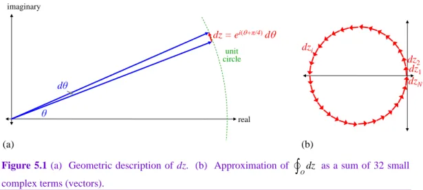
5 Complex Analytic Functions ...65
Residues ...66
Contour Integrals ...67
Evaluating Integrals ...67
Choosing the Right Path: Which Contour? ...70
Evaluating Infinite Sums ...75
Multi-valued Functions ...77
6 Conceptual Linear Algebra ...79
Matrix Multiplication ...79
Cramer’s Rule ...81
Area and Volume as a Determinant ...82
The Jacobian Determinant and Change of Variables ...83
Expansion by Cofactors ...85
Proof That the Determinant Is Unique ...87
Getting Determined ...88
Advanced Matrices ...89
Getting to Home Basis ...89
Diagonalizing a Self-Adjoint Matrix ...90
Contraction of Matrices ...92
Trace of a Product of Matrices ...92
Linear Algebra Briefs ...93
7 Introduction to Probability, Statistics, and Data Analysis ...94
Probability and Random Variables ...94
Precise Statement of the Question Is Critical ...95
How to Lie With Statistics ...96
Choosing Wisely: An Informative Puzzle ...96
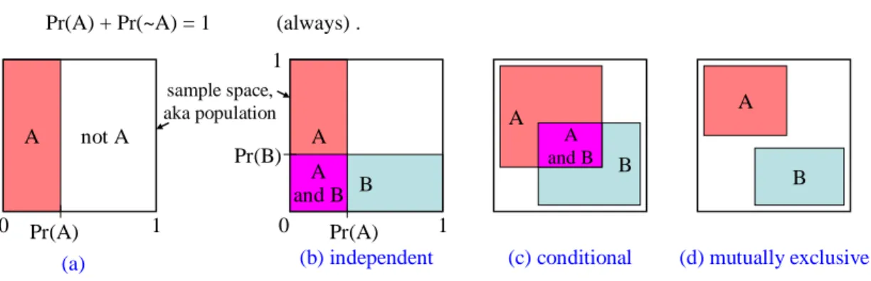
Multiple Events ...97
Combining Probabilities ...98
To B, or To Not B? ...100
Continuous Random Variables and Distributions ...102
Populations ...102
Population Variance ...103
Population Standard Deviation ...103
New Random Variables From Old Ones ...104
Some Distributions Have Infinite Variance, or Infinite Average ...105
Samples and Parameter Estimation ...106
Why Do We Use Least Squares, and Least Chi-Squared (χ2)? ...106
Average, Variance, and Standard Deviation ...107
Functions of Random Variables ...111
Statistically Speaking: What Is The Significance of This? ...111
Predictive Power: Another Way to Be Significant, but Not Important ...114
Unbiased vs. Maximum-Likelihood Estimators ...114
Correlation and Dependence ...116
Independent Random Variables are Uncorrelated ...117
r You Serious? ...118
Statistical Analysis Algebra ...119
The Average of a Sum: Easy? ...119
The Average of a Product...120
Variance of a Sum ...120
Covariance Revisited ...120
Capabilities and Limits of the Sample Variance ...121
How to Do Statistical Analysis Wrong, and How to Fix It ...123
Introduction to Data Fitting (Curve Fitting) ...124
Goodness of Fit ...125
Guidance Counselor: Computer Code to Fit Data ...129
8 Multiple Linear Regression ...133
Review of Multiple Linear Regression ...133
We Fit to the Predictors, Not the Independent Variable ...133
Homoskedastic Case: All Measurements Have the Same Uncertainty ...136
The Raw Sum-of-Squares Identity ...137
The Geometric View of a Least-Squares Fit ...138
Algebra and Geometry of the Sum-of-Squares Identity ...140
The ANOVA Sum-of-Squares Identity ...140
Subtracting DC Before Analysis: Just Say No ...142
Fitting to Orthonormal Functions ...143
Hypothesis Testing with the Sum of Squares Identity ...143
Introduction to Analysis of Variance (ANOVA) ...143
The Temperature of Liberty ...144
The F-test: The Decider for Zero Mean Gaussian Noise ...148
Coefficient of Determination and Correlation Coefficient ...149
9 Uncertainty Weighted Linear Regression ...152
Be Sure of Your Uncertainty ...152
Average of Uncertainty Weighted Data ...152
Variance and Standard Deviation of Uncertainty Weighted Data ...154
Normalized weights ...156
Numerically Convenient Weights ...157
Uncertainty Weighted Straight-Line Fit ...157
Transformation to Equivalent Homoskedastic Measurements ...157
Linear Regression with Individual Uncertainties ...159
Linear Regression With Uncertainties and the Sum-of-Squares Identity ...160
Hypothesis Testing a Model in Linear Regression with Uncertainties ...165
10 Practical Considerations for Data Analysis ...166
Rules of Thumb ...166
Signal to Noise Ratio (SNR) ...166
Computing SNR From Data ...167
Spectral Method of Estimating SNR ...168
Fitting Models To Histograms (Binned Data) ...169
Reducing the Effect of Noise ...172
Data With a Hard Cutoff: When Zero Just Isn’t Enough ...174
Filtering and Data Processing for Equally Spaced Samples ...175
Finite Impulse Response Filters (aka Rolling Filters) and Boxcars ...175
Use Smooth Filters (not Boxcars) ...176
11 Fourier Transforms and Digital Signal Processing ...177
Model of Digitization and Sampling ...178
Complex Sequences and Complex Fourier Transform ...178
Basis Functions and Orthogonality ...181
Real Sequences...182
Normalization and Parseval’s Theorem ...183
Continuous and Discrete, Finite and Infinite ...185
White Noise and Correlation ...185
Why Oversampling Does Not Improve Signal-to-Noise Ratio ...185
Filters TBS?? ...186
What Happens to a Sine Wave Deferred? ...186
Nonuniform Sampling and Arbitrary Basis Functions ...188
Don’t Pad Your Data, Even for FFTs...190
Two Dimensional Fourier Transforms ...191
Note on Continuous Fourier Series and Uniform Convergence ...191
Fourier Transforms, Periodograms, and Lomb-Scargle ...192
The Discrete Fourier Transform vs. the Periodogram ...193
Practical Considerations ...194
The Lomb-Scargle Algorithm ...195
The Meaning Behind the Math ...196
Bandwidth Correction (aka Bandwidth Penalty) ...200
Analytic Signals and Hilbert Transforms ...203
Summary ...208
12 Period Finding ...210
Overview of Period Finding Algorithms ...211
References ...211
Phase Dispersion Minimization ...211
PDM Algorithm ...212
PDM On Data With Trends ...216
Subharmonic Response ...217
Harmonic response ...217
Spectral window function...218
References ...218
13 Numerical Analysis ...219
Round-Off Error, And How to Reduce It ...219
How To Extend Precision In Sums Without Using Higher Precision Variables ...220
Numerical Integration ...221
Sequences of Real Numbers ...221
Root Finding ...221
Simple Iteration Equation...221
Newton-Raphson Iteration ...223
Pseudo-Random Numbers ...226
Generating Gaussian Random Numbers ...227
Generating Poisson Random Numbers...227
Generating Useful, But More Challenging, Random Numbers ...228
Exact Polynomial Fits ...229
14 Computer Math Internals ...231
Digital Integer Arithmetic: Two’s Complement ...231
Hexadecimal ...232
Digital Floating Point ...233
How Far Can I Go? ...233
How Many Digits Do I Get, 6 or 9? ...233
How many digits do I need? ...234
Emulate vs. Simulate ...234
Programming Guidance for Floating Point ...235
IEEE Floating Point ...236
Precision in Binary and Decimal ...243
The Big ULP ...243
Round and Round ...244
Underflow ...245
References ...246
15 Scientific Programming: Discovering Efficiency ...247
Software Development Efficiency ...247
Some Do’s and Don’t’s ...247
Considerations on Development Efficiency and Languages ...248
Sophistication Follows Function ...248
Engineering vs. Programming ...249
Object Oriented Programming ...249
The Best of Times, the Worst of Times: Run-time Efficiency ...250
Example Using Matrix Addition ...251
Memory Consumption vs. Run Time: Cache as Cache Can ...255
Cache Withdrawal: Making the Most of Reference Locality ...257
Data Structures for Efficient Cache Use ...258
Algorithms for Efficient Cache Use ...259
Cache Optimization Summary ...259
Virtual Memory and Page Locality ...259
Considerations on Run-Time Efficiency and Languages ...261
Approach ...262
Two Physical Examples ...262
Magnetic Susceptibility ...262
Mechanical Strain...266
When Is a Matrix Not a Tensor? ...268
Heading In the Right Direction ...268
Some Definitions and Review ...268
Vector Space Summary ...269
When Vectors Collide ...270
“Tensors” vs. “Symbols”...271
Notational Nightmare ...271
Tensors? What Good Are They? ...271
A Short, Complicated Definition...271
Building a Tensor ...272
Tensors in Action ...273
Tensor Fields ...274
Dot Products and Cross Products as Tensors ...274
The Danger of Matrices...276
Reading Tensor Component Equations ...276
Adding, Subtracting, Differentiating Tensors ...277
Higher Rank Tensors ...277
Tensors In General ...279
Change of Basis: Transformations ...279
Matrix View of Basis Transformation ...280
Geometric (Coordinate-Free) Dot and Cross Products ...281
Non-Orthonormal Systems: Contravariance and Covariance...283
Dot Products in Oblique Coordinates ...283
Covariant Components of a Vector ...284
Example: Classical Mechanics with Oblique Generalized Coordinates ...285
What Goes Up Can Go Down: Duality of Contravariant and Covariant Vectors ...288
The Real Summation Convention ...289
Transformation of Covariant Indexes ...289
Indefinite Metrics: Relativity ...290
Is a Transformation Matrix a Tensor? ...290
How About the Pauli Vector? ...291
Cartesian Tensors ...291
The Real Reason Why the Kronecker Delta Is Symmetric ...292
Tensor Appendices ...292
Pythagorean Relation for 1-forms ...292
Geometric Construction Of The Sum Of Two 1-Forms: ...293
“Fully Anti-symmetric” Symbols Expanded ...294
Metric? We Don’t Need No Stinking Metric! ...295
References: ...297 17 Differential Geometry ...298 Manifolds ...298 Coordinate Bases ...298 Covariant Derivatives ...300 Christoffel Symbols ...302 Visualization of n-Forms ...303
Review of Wedge Products and Exterior Derivative...303
Wedge Products ...303
Tensor Notation ...304
1D ...304
2D ...304
18 Math That’s Fun and Interesting ...307
Math Tricks That Come Up A Lot ...307
The Gaussian Integral ...307
Math Tricks That Are Fun and Interesting ...307
Phasors ...308
Miserables Coset ...308
Public Key Cryptography on a Hand Calculator...309
Public Key Cryptography Overview ...309
RSA Overview ...310
Examples of Relevant Modular Arithmetic ...310
Application to RSA Cryptosystem ...312
Raising to Large Powers ...312
Finding the Maximum Period ...313
Finding Large Primes: It’s a Gamble ...313
RSA By the Numbers ...313
Practical Note on Efficiency ...314
Digital Signatures ...314 Vulnerabilities ...314 Secret Message ...315 References ...315 19 Appendices ...316 References ...316 Glossary ...317 Formulas...321 Index ...322
a
cos a
sin a
1
un
it
tan a
cot a
sec a
cs
c
a
O
A
B
C
D
a
Copyright 2001 Inductive Logic. All rights reserved.
cos a
From OAD:
sin
=
opp
/ hyp
cos
=
adj
/ hyp
sin
2+
cos
2= 1
From OAB:
tan
=
opp
/ adj
tan
2+ 1 =
sec
2(and with OAD)
tan
=
sin
/
cos
sec
=
hyp
/ adj = 1 /
cos
From OAC:
cot
=
adj
/ opp
cot
2+ 1 =
csc
2(and with OAD)
cot
=
cos
/
sin
1
Introduction
Mathematical Physics, or Physical Mathematics?
Is There Another Kind of Physics? Mathematical Physics is devoted to the natural emergence of mathematics from our curiosity about the universe around us. All physics is mathematical, but Mathematical Physics illustrates that math is not abstract, or capricious, but an inescapable part of the natural world. Despite its humble beginnings rooted in conceptual understanding and the practice of science, many find that Mathematical Physics holds a beauty and fascination all its own.
As with all “Funky” notes, we emphasize the physical meaning of the underlying concepts. For example, we stress a coordinate-free, geometric approach to vector operations.
Why Physicists and Mathematicians Argue
Physics goals and mathematics goals are antithetical. Physics seeks to ascribe meaning to mathematics that describe the world, to “understand” it, physically. Mathematics seeks to strip the equations of all physical meaning, and view them in purely abstract terms. These divergent goals set up a natural conflict between the two camps. Each goal has its merits: the value of physics is (or should be) self-evident; the value of mathematical abstraction, separate from any single application, is generality: the results can be used on a wide range of applications.
Why Funky?
The purpose of the “Funky” series of documents is to help develop an accurate physical, conceptual, geometric, and pictorial understanding of important physics topics. We focus on areas that don’t seem to be covered well in most texts. The Funky series attempts to clarify those neglected concepts, and others that seem likely to be challenging and unexpected (funky?). The Funky documents are intended for serious students of physics; they are not “popularizations” or oversimplifications.
Physics includes math, and we’re not shy about it, but we also don’t hide behind it. Without a conceptual understanding, math is gibberish.
This work is one of several aimed at graduate and advanced-undergraduate physics students. Go to our web page (in the page header) for the latest versions of the Funky Series, and for contact information. We’re looking for feedback, so please let us know what you think.
How to Use This Document
This work is not a text book.
There are plenty of those, and they cover most of the topics quite well. This work is meant to be used with a standard text, to help emphasize those things that are most confusing for new students. When standard presentations don’t make sense, come here.
You should read all of this introduction to familiarize yourself with the notation and contents. After that, this work is meant to be read in the order that most suits you. Each section stands largely alone, though the sections are ordered logically. Simpler material generally appears before more advanced topics. You may read it from beginning to end, or skip around to whatever topic is most interesting. The “Shorts” chapter is a diverse set of very short topics, meant for quick reading.
If you don’t understand something, read it again once, then keep reading. Don’t get stuck on one thing. Often, the following discussion will clarify things.
Thank You
I owe a big thank you to many professors at both SDSU and UCSD, for their generosity even when I wasn’t a real student: Dr. Herbert Shore, Dr. Peter Salamon, Dr. Arlette Baljon , Dr. Andrew Cooksy, Dr. George Fuller, Dr. Tom O’Neil, Dr. Terry Hwa, and others.
Scope
What This Text Covers
This text covers some of the unusual or challenging concepts in graduate mathematical physics. It is also very suitable for upper-division undergraduate level, as well. We expect that you are taking or have taken such a course, and have a good text book. Funky Mathematical Physics Concepts supplements those other sources.
What This Text Doesn’t Cover
This text is not a mathematical physics course in itself, nor a review of such a course. We do not cover all basic mathematical concepts; only those that are very important, unusual, or especially challenging (funky?).
What You Already Know
This text assumes you understand basic integral and differential calculus, and partial differential equations. Further, it assumes you have a mathematical physics text for the bulk of your studies, and are using Funky Mathematical Physics Concepts to supplement it.
Notation
Sometimes the variables are inadvertently not written in italics, but I hope the meanings are clear. ?? refers to places that need more work.
TBS To be supplied (one hopes) in the future.
Interesting points that you may skip are “asides,” shown in smaller font and narrowed margins. Notes to myself may also be included as asides.
Common misconceptions are sometimes written in dark red dashed-line boxes.
Formulas: We write the integral over the entire domain as a subscript “∞”, for any number of dimensions:
3
1-D: dx 3-D: d x
Evaluation between limits: we use the notation [function]ab to denote the evaluation of the function between a and b, i.e.,
[f(x)]ab ≡ f(b) – f(a). For example, ∫ 01 3x2 dx = [x3]01 = 13 - 03 = 1. We write the probability of an event as “Pr(event).”
Column vectors: Since it takes a lot of room to write column vectors, but it is often important to distinguish between column and row vectors, I sometimes save vertical space by using the fact that a column vector is the transpose of a row vector:
(
, , ,)
T a b a b c d c d = Random variables: We use a capital letter, e.g. X, to represent the population from which instances of a random variable, x (lower case), are observed. In a sense, X is a representation of the PDF of the random variable, pdfX(x).
We denote that a random variable X comes from a population PDF as: X pdfX, e.g.: X χ2(n). To denote that X is a constant times a random variable from pdfY, we write: X k pdfY, e.g. X k χ2(n).
For Greek letters, pronunciations, and use, see Quirky Quantum Concepts. Other math symbols: Symbol Definition
for all there exists such that iff if and only if
proportional to. E.g., a b means “a is proportional to b” ⊥ perpendicular to
therefore
of the order of (sometimes used imprecisely as “approximately equals”) is defined as; identically equal to (i.e., equal in all cases)
implies → leads to
tensor product, aka outer product direct sum
In mostly older texts, German type (font: Fraktur) is used to provide still more variable names:
Latin
German Capital
German
Lowercase Notes
A
A
a
Distinguish capital from U, VB
B
b
C
C
c
Distinguish capital from E, GD
D
d
Distinguish capital from O, QE
E
e
Distinguish capital from C, GF
F
f
G
G
g
Distinguish capital from C, EH
H
h
I
I
i
Capital almost identical to JJ
J
j
Capital almost identical to IK
K
k
L
L
l
N
N
n
O
O
o
Distinguish capital from D, QP
P
p
Q
Q
q
Distinguish capital from D, OR
R
r
Distinguish lowercase from xS
S
s
Distinguish capital from C, G, ET
T
t
Distinguish capital from IU
U
u
Distinguish capital from A, VV
V
v
Distinguish capital from A, UW
W
w
Distinguish capital from MX
X
x
Distinguish lowercase from rY
Y
y
2
Random Short Topics
I Always Lie
Logic, and logical deduction, are essential elements of all science. Too many of us acquire our logical reasoning abilities only through osmosis, without any concrete foundation. Unfortunately, two of the most commonly given examples of logical reasoning are both wrong. I found one in a book about Kurt Gödel (!), the famous logician.
Fallacy #1: Consider the statement, “I always lie.” Wrong claim: this is a contradiction, and cannot be either true or false. Right answer: this is simply false. The negation of “I always lie” is not “I always tell the truth;” it is “I don’t always lie,” equivalent to “I at least sometimes tell the truth.” Since “I always lie” cannot be true, it must be false, and it must be one of my (exceedingly rare) lies.
Fallacy #2: Consider the statement, “The barber shaves everyone who doesn’t shave himself. Who shaves the barber?” Wrong answer: it’s a contradiction, and has no solution. Right answer: the barber shaves himself. The original statement is about people who don’t shave themselves; it says nothing about people who do shave themselves. If A then B; but if not A, then we know nothing about B. The barber does shave everyone who does not shave himself, and he also shaves one person who does shave himself: himself. To be a contradiction, the claim would need to be something like, “The barber shaves all and only those who don’t shave themselves.”
Logic matters.
What’s Hyperbolic About Hyperbolic Sine?
x
sinh a
area = a/2 y y = x x2– y2= 1cos a
sin a
x2+ y2= 1 x y area = a/2 1 un itcosh a
1 unita
From where do the hyperbolic trigonometric functions get their names? By analogy with the circular functions. We usually think of the argument of circular functions as an angle, a. But in a unit circle, the area covered by the angle a is a / 2 (above left):
2 ( 1) 2 2 a a area r r = = = .
Instead of the unit circle, x2 + y2 = 1, we can consider the area bounded by the x-axis, the ray from the origin, and the unit hyperbola, x2 – y2 = 1 (above right). Then the x and y coordinates on the curve are called the hyperbolic cosine and hyperbolic sine, respectively. Notice that the hyperbola equation implies the well-known hyperbolic identity:
2 2 2 2
cosh , sinh , 1 cosh sinh 1
x= a y= a x −y = − = .
Proving that the area bounded by the x-axis, ray, and hyperbola satisfies the standard definition of the hyperbolic functions requires evaluating an elementary, but tedious, integral: (?? is the following right?)
2 1 2 2 1 2 2 2 2 2 3 1 1 1 1 1 Use: 1 2 2 1 2 1
For the integral, let sec , tan sec sec 1 tan
sin
1 sec 1 tan sec tan sec
cos x x x x x x a area xy y dx y x a x x x dx x dx d y x dx d d d = = − = − = − − − = = = − = − = − = =
We try integrating by parts (but fail):
2
2 3
1
1 1
tan sec tan sec , sec
tan sec sec tan sec
x x x U dV d dU d V d UV V dU d = = = = = − = −
This is too hard, so we try reverting to fundamental functions sin( ) and cos( ):
(
)
3 2 2 2 3 2 2 1 1 1 1 2 1 1 1 2 1sin cos sin cos , cos
2
sin sin sin
2 2 2 cos cos Use: sec tan
cos cos cos
sec ln sec tan ln 1
ln 1 ln1 x x x x x x x U dV d dU d V d UV V dU d xy xy d xy xy x x xy x x − − − = = = = = − = − = = = − = − + = − + − = − + − −
2 2 2 ln 1 ln 1 1 a a xy xy x x x x e x x = − + + − = + − = + −Solve for x in terms of a, by squaring both sides:
(
)
(
)
2 2 2 2 2 2 2 1 1 2 1 1 2 1 1 2 2 cosh 2 a a a e a a a a a a e x x x x x x x xe e xe e e e e x x a − − = + − + − = + − − = − + = + + = =The definition for sinh follows immediately from:
(
)
2 2 2 2 2 2 2 2 2 2 2 cosh sinh 1 1 2 2 sinh 1 1 2 4 4 4 2 a a a a a a a a a a x y y x e e e e e e e e e e a y − − − − − − = − = = − − + + + − + − = − = − = = = Basic Calculus You May Not Know
Amazingly, many calculus courses never provide a precise definition of a “limit,” despite the fact that both of the fundamental concepts of calculus, derivatives and integrals, are defined as limits! So here we go:
Basic calculus relies on 4 major concepts: 1. Functions
2. Limits 3. Derivatives 4. Integrals
1. Functions: Briefly, (in real analysis) a function takes one or more real values as inputs, and produces one or more real values as outputs. The inputs to a function are called the arguments. The simplest case is a real-valued function of a real-valued argument e.g., f(x) = sin x. Mathematicians would write (f : R1 → R1), read “f is a map (or function) from the real numbers to the real numbers.” A function which produces more than one output may be considered a vector-valued function.
2. Limits: Definition of “limit” (for a real-valued function of a single argument, f : R1 → R1):
L is the limit of f(x) as x approaches a, iff for every ε > 0, there exists a δ (> 0) such that |f(x) – L| < ε whenever 0 < |x – a| < δ. In symbols:
lim ( ) iff 0, such that ( ) whenever 0
x a
L f x f x L x a
→
= − − .
This says that the value of the function at a doesn’t matter; in fact, most often the function is not defined at a. However, the behavior of the function near a is important. If you can make the function arbitrarily close to some number, L, by restricting the function’s argument to a small neighborhood around a, then L is the limit of f as x approaches a.
Surprisingly, this definition also applies to complex functions of complex variables, where the absolute value is the usual complex magnitude.
Example: Show that 2 1 2 2 lim 4 1 x x x → − = − .
Solution: We prove the existence of δ given any ε by computing the necessary δ from ε. Note that for
2 2 2 1, 2( 1) 1 x x x x − = +
− . The definition of a limit requires that 2 2 2 4 whenever 0 1 1 x x x − − − − .
We solve for x in terms of ε, which will then define δ in terms of ε. Since we don’t care what the function is at x = 1, we can use the simplified form, 2(x + 1). When x = 1, this is 4, so we suspect the limit = 4. Proof:
2( 1) 4 2 ( 1) 2 1 1 1
2 2 2
x+ − x+ − x− or − + . x
So by setting δ = ε/2, we construct the required δ for any given ε. Hence, for every ε, there exists a δ satisfying the definition of a limit.
3. Derivatives: Only now that we have defined a limit, can we define a derivative:
0 ( ) ( ) '( ) lim x f x x f x f x x → + − .
4. Integrals: A simplified definition of an integral is an infinite sum of areas under a function divided into equal subintervals (Figure 2.1, left):
(
)
1( ) lim (simplified definition)
N b a N i x b a i f x dx f b a N N → = − −
.For practical physics, this definition is fine. For mathematical preciseness, the actual definition of an integral is the limit over any possible set of subintervals [ref??], so long as the maximum of the subinterval size goes to zero. This maximum size is called “the norm of the subdivision,” written as ||Δxi||:
( )
01
( ) lim (precise definition)
i N b i i a x i f x dx f x x → =
.Figure 2.1 (Left) Simplified definition of an integral as the limit of a sum of equally spaced samples. (Right) Precise definition requires convergence for arbitrary, but small, subdivisions.
Why do mathematicians require this more precise definition? It’s to avoid bizarre functions, such as: f(x) is 1 if x is rational, and zero if irrational. This means f(x) toggles wildly between 1 and 0 an infinite number of times over any interval. However, with the simplified definition of an integral, the following are both well defined:
3.14
0 f x dx( ) 3.14, and 0 f x dx( ) 0 (with simplified definition of integral)
= =
.In contrast, with the mathematically precise definition of an integral, both integrals are undefined. (There are other types of integrals defined, but they are beyond our scope.)
The Product Rule
Given functions U(x) and V(x), the product rule (aka the Leibniz rule) says that for differentials,
( )
d UV =U dV+V dU. (2.1)
When U and V are functions of x, we have:
( ) ( )
( ) '( ) ( ) '( )d U x V x =U x V x dx V x U x dx+ .
This leads to integration by parts, which is mostly known as an integration tool, but it is also an important theoretical (analytic) tool, and the essence of Legendre transformations.
Integration By Pictures
We assume you are familiar with integration by parts (IBP) as a tool for performing indefinite integrals. We start with a brief overview, and then discuss a specific example in detail. IBP takes a non-trivial integral into an expression with a different integral, which may be easier to perform analytically:
( ) ( ), ( )
f x dx = U dV =UV− V dU where UU x V V x
are parametric functions of x. The above comes directly from the product rule (2.1): U dV =d UV
( )
−V dU , and integrate both sides. Inserting limits of integration makes for a simple illustration of the formula’s meaning (Figure 2.2a), but a slightly tedious equation:
( )( )
big rectangle sma ) ll rect ( ( ) angle ( ) ( ) ( ) ( ) ( ) ( ) ( ) ( ), ( ) . b V b U b U a x V a b U b a a U a f x dx UV V dU U b V b U a V a where U U x V V x V d U Vd U − = = = − − −
The figure plots U vs. V, where we’ve chosen U and V to be increasing parametric functions of x. In practice, the RHS of (2.2) is usually written in terms of x as:
( ) '( ) ( ) ( )b ( ) '( ) . dV d b a U b x a a U x V x dx= U x V x = − V x U x dx
(2.3)Note that x is the original integration variable (not U or V), so all the limits of integration are the original x = a to x = b.
In practice, our job is to integrate f(x) dx by finding functions U(x) and V(x) such that the resulting integral on the RHS of (2.3) is simpler than the original f(x) dx. As a specific example, consider:
( ) sin f x x x dx
.Figure 2.2b illustrates the definite integral 2.7 1 f x dx( )
to scale, with uniform representative intervals dx. U (a) (b) (c) f(x) V x dx dV V U V(a) V(b) U(a) U(b) U(b)V(b) ∫U dV U(a)V(a) ∫V dUFigure 2.2 (a) Schematic identification of significant features of IBP. (b) To scale: the original integral can be reconsidered as (c) an integral of U dV; the areas are equal. U and V are parametric functions of x; dV is a function of x and dx. As shown, when the dx are uniform, the dV are not.
This integral is not immediate, so we can try integration by parts, though there is no guarantee that it will work. In this example, there are three ways of choosing U(x) and V(x):
(
)
2
( ) sin , cos sin , ( )
( ) , sin , ( ) cos ( ) sin , cos , ( ) / 2 U x x x dV dx dU x x x dx V x x U x x dV x dx dU dx V x x U x x dV x dx dU x dx V x x = = = + = = = = = − = = = =
More complicated integrals will have more choices for U(x) and V(x). It is hard to know ahead of time which choice (or choices) will succeed. However, looking at the RHS of (2.3), we see that it multiplies V and the derivative of U. Looking at our 3 choices above, on the RHS of the arrows, we find the two factors V dU that we would be faced with integrating:
• the second choice has dU = dx, which literally could not be simpler, and V dU integrates easily; • the last choice has dU = cos x dx, which isn’t bad, but V dU cannot be easily integrated.
Thus our best guess is the second choice (often, the simplest dU is a good choice). Figure 2.2c illustrates U dV
to scale; U and V are parametric functions of x; dV is a function of x and dx. Then:sin cos cos cos sin
UV V dU
x x dx = −x x− − x dx = −x x+ x
.We check by differentiating the RHS above, which yields the original integrand.
Note that when the dx in Figure 2.2b are uniform, the dV in Figure 2.2c are not. However, all the dV go to zero when the dx do, so the integral of U dV is still valid.
The term
( ) ( )
b aU x V x is called the “boundary term,” or sometimes the “surface term.” U U(a) = 0 U(b) V(a) ∫U dV = −∫V dU integration direction V(b) = 0 V U(a) U(b) Vmax V(a) = V(b) = 0 ∫V dU > 0 ∫1U dV 1 2 U V (a) (b) ∫U dV < 0 ∫U dV < 0
Figure 2.3 Two more cases of integration by parts: (a) V(x) decreasing to 0. (b) V(x) progressing from zero, to finite, and back to zero.
More advanced cases of Integration By Parts: Figure 2.3a illustrates another common case: one in which the boundary term UV is zero. In this example, UV = 0 at x = a because U(a) = 0, and at x = b because V(b) = 0. This means V(x) decreases as x increases. Viewed as
U dV , all the dV < 0. The shaded “area” is therefore negative. Viewed (sideways) as
V dU, all the dU > 0 and the shaded area is positive. Thus:
( ) b 0 a f x dx = U dV = − V dU when UV =
, in agreement with (2.3).Figure 2.3b shows the case where UV = 0 at x = a and b, because one of U(x) or V(x) starts and ends at 0. For illustration, we chose V(a) = V(b) = 0. Then the boundary term is zero, and we again have:
( ) ( )
b 0 b x a x b x a a U x V x = U dV V dU = = =
= −
.For V(x) to start and end at zero, V(x) must grow with x to some maximum, Vmax, and then decrease back to 0. For simplicity, we assume U(x) is always increasing. The V dU integral is the blue striped area to the left of the curve, and is > 0. The U dV integral is the area under the curves. We break the U dV integral into two parts: path 1, leading up to Vmax, and path 2, going back down from Vmax to zero. The integral from 0 to Vmax (path 1) is the red striped area; the integral from Vmax back down to 0 (path 2) is the negative of the entire (blue + red) striped area. Then the blue shaded region is the difference (< 0):
(2) the (blue + red) area below path 2, where dV is negative because V(x) is decreasing. Thus
0
U dV
:max max max
max 0 0 1 2 0 0 1 2 1 2 . V V V V
path path p path
V V V V p p b x t a a h ath ath U dV U U dV V dU d dV U dV U V = = = + = = = + = − = −
Theoretical Importance of IBP
Besides being an integration tool, an important theoretical consequence of IBP is that the variable of integration is changed, from dV to dU. Many times, one differential is unknown, but the other is known:
Given an integral, integration by parts allows you to exchange a differential that cannot be directly evaluated, even in principle, in favor of one that can.
The classic example of this is deriving the Euler-Lagrange equations of motion from the principle of stationary action. The action of a dynamic system is defined by:
( ( ), ( ))
S
L q t q t dt,where the lagrangian is a given function of the trajectory q(t). Stationary action means that the action does not change (to first order) for small changes in the trajectory. I.e., given a small variation in the trajectory, δq(t): 0 ( , ) L L S L q q q q dt S q q dt q q = = + + − = +
.The quantity in brackets involves both δq(t) and its time derivative, q t( ). We are free to vary δq(t) arbitrarily, but that fully determines q t( ). We cannot vary both δq and q separately. We also know that δq(t) = 0 at its endpoints, but q t( ) is unconstrained at its endpoints. Therefore, it would be simpler if the quantity in brackets were written entirely in terms of δq(t), and not in terms of q. This is easy:
Use q d q: S 0 L q L d q dt dt q q dt = = = +
.Now in the second term, IBP allows us to eliminate the time derivative of δq(t) (which is unconstrained) in favor of the time derivative of L/q (which we can easily find, since L q q( , ) is given). Therefore, this is a good trade. Integrating the 2nd term in brackets by parts gives:
0 ' Let , . , ( ) t f V U t L d L d U dU dt dV q dt V q q d dt q d L dt L t UV V d dt U q q t q q = = = = = = = − =
' . U V d L dt q dt q −
The boundary term is zero because δq(t) is zero at both endpoints. The variation in action δS is now:
0 ( ) L d L S q dt q t q dt q = − =
.The only way δS = 0 can be satisfied for any δq(t) is if the quantity in brackets is identically 0. Thus IBP has led us to an important theoretical conclusion: the Euler-Lagrange equation of motion.
This fundamental result has nothing to do with evaluating a specific difficult integral. IBP: it’s not just for hard integrals any more.
Delta Function Surprise: Coordinates Matter
Rarely, one needs to consider the 3D δ-function in coordinates other than rectangular. The coordinate-free 3D δ-function is written δ3(r – r’). For example, in 3D Green functions, whose definition depends on a δ3-function, it may be convenient to use cylindrical or spherical coordinates. In these cases, there are some
unexpected consequences [Wyl p280]. This section assumes you understand the basic principle of a 1D and 3D δ-function. (See the introduction to the delta function in Quirky Quantum Concepts.)
Recall the defining property of δ3(r - r’):
3 3( ') 1 ' ( " ") 3 3( ') ( ) ( ')
d for all d f f
− = − =
r r r r
r r r r r .The above definition is “coordinate free,” i.e. it makes no reference to any choice of coordinates, and is true in every coordinate system. As with Green functions, it is often helpful to think of the δ-function as a function of r, which is zero everywhere except for an impulse located at r’. As we will see, this means that it is properly a function of r and r’ separately, and should be written as δ3(r, r’) (like Green functions are).
Rectangular coordinates: In rectangular coordinates, however, we now show that we can simply break up δ3(x, y, z) into 3 components. By writing (r – r’) in rectangular coordinates, and using the defining integral above, we get: 3 3 ' ( ', ', ') ( ', ', ') 1 ( ', ', ') ( ') ( ') ( ') . x x y y z z dx dy dz x x y y z z x x y y z z x x y y z z − − − − − − − − − − = − − − = − − −
r rIn rectangular coordinates, the above shows that we do have translation invariance, so we can simply write: 3( , , )x y z ( ) ( ) ( )x y z
= .
In other coordinates, we do not have translation invariance. Recall the 3D infinitesimal volume element in 4 different systems: coordinate-free, rectangular, cylindrical, and spherical coordinates:
3 2sin
d r=dx dy dz=r dr d dz =r dr d d .
The presence of r and θ imply that when writing the 3D δ-function in non-rectangular coordinates, we must include a pre-factor to maintain the defining integral = 1. We now show this explicitly.
Cylindrical coordinates: In cylindrical coordinates, for r > 0, we have (using the imprecise notation of [Wyl p280]): 2 3 0 0 3 ' ( ', ', ') ( ', ', ') 1 1 ( ', ', ') ( ') ( ') ( '), ' 0 ' r r z z dr d dz r r r z z r r z z r r z z r r − − = − − − − − − = − − − = − − −
r rNote the 1/r' pre-factor on the RHS. This may seem unexpected, because the pre-factor depends on the location of δ3( ) in space (hence, no radial translation invariance). The rectangular coordinate version of δ3( ) has no such pre-factor. Properly speaking, δ3( ) isn’t a function of r – r'; it is a function of r and r' separately.
In non-rectangular coordinates, δ3( ) does not have translation invariance,
and includes a pre-factor which depends on the position of δ3( ) in space, i.e. depends on r’.
At r' = 0, the pre-factor blows up, so we need a different pre-factor. We’d like the defining integral to be 1, regardless of , since all values of are equivalent at the origin. This means we must drop the δ( – ’), and replace the pre-factor to cancel the constant we get when we integrate out :
2 3 0 0 3 0 ( ', ', ') 1, ' 0 1 ( ', ', ') ( ) ( '), ' 0, 2 assuming that ( ) 1. dr d dz r r r z z r r r z z r z z r r dr r − − − − = = − − − = − = =
This last assumption is somewhat unusual, because the δ-function is usually thought of as symmetric about 0, where the above radial integral would only be ½. The assumption implies a “right-sided” δ-function, whose entire non-zero part is located at 0+. Furthermore, notice the factor of 1/r in δ(r – 0, z – z’). This factor blows up at r = 0, and has no effect when r ≠ 0. Nonetheless, it is needed because the volume element r dr d dz goes to zero as r → 0, and the 1/r in δ(r – 0, z – z’) compensates for that.
Spherical coordinates: In spherical coordinates, we have similar considerations. First, away from the origin, r’ > 0: 2 2 3 0 0 0 3 2 sin ( ', ', ') 1 1 ( ', ', ') ( ') ( ') ( '), ' 0 . [Wyl 8.9.2 p280] ' sin ' dr d d r r r r r r r r r − − − = − − − = − − −
Again, the pre-factor depends on the position in space, and properly speaking, δ3( ) is a function of r, r’, θ, and θ’ separately, not simply a function of r – r’ and θ – θ’. At the origin, we’d like the defining integral to be 1, regardless of or θ. So we drop the δ( – ’) δ(θ – θ’), and replace the pre-factor to cancel the constant we get when we integrate out and θ:
2 2 3 0 0 0 3 2 0 sin ( 0, ', ') 1, ' 0 1 ( 0, ', ') ( ), ' 0, 4 assuming that ( ) 1. dr d d r r r r r r r dr r − − − = = − − − = = =
Again, this definition uses the modified δ(r), whose entire non-zero part is located at 0+. And similar to the cylindrical case, this includes the 1/r2 factor to preserve the integral at r = 0.
2D angular coordinates: For 2D angular coordinates θ and , we have: 2 2 0 0 2 sin ( ', ') 1, ' 0 1 ( ', ') ( ') ( '), ' 0 . sin ' d d − − = − − = − −
Once again, we have a special case when θ’ = 0: we must have the defining integral be 1 for any value of . Hence, we again compensate for the 2π from the integral:
2 2 0 0 2 sin ( ', ') 1, ' 0 1 ( 0, ') ( ), ' 0 . 2 sin d d − − = = − − = =
Spherical Harmonics Are Not Harmonics
See Funky Electromagnetic Concepts for a full discussion of harmonics, Laplace’s equation, and its solutions in 1, 2, and 3 dimensions. Here is a brief overview.
Spherical harmonics are the angular parts of solid harmonics, but we will show that they are not truly “harmonics.” A harmonic is a function which satisfies Laplace’s equation:
2
( ) 0
r = , with r typically in 2 or 3 dimensions.
Solid harmonics are 3D harmonics: they solve Laplace’s equation in 3 dimensions. For example, one form of solid harmonics separates into a product of 3 functions in spherical coordinates:
( )
(
)
(
)
( )(
)
1 1( , , ) ( ) ( ) ( ) (cos ) sin cos
( ) is the radial part,
( ) (cos ) is the polar angle part, the associated Legendre functions,
( ) sin cos is the azimuthal part .
l l l l l l l l l l l lm l l r R r P Q A r B r P m C m D m where R r A r B r P P Q C m D m − + − + = = + + = + = = +
The spherical harmonics are just the angular (θ, ) parts of these solid harmonics. But notice that the angular part alone does not satisfy the 2D Laplace equation (i.e., on a sphere of fixed radius):
2 2 2 2 2 2 2 2 2 2 2 2 1 1 1
sin , but for fixed :
sin sin 1 1 1 sin . sin sin r r r r r r r r = + + = +
However, direct substitution of spherical harmonics into the above Laplace operator shows that the result is not 0 (we let r = 1). We proceed in small steps:
2 2 2 ( ) sin cos ( ) ( ) Q C m D m Q m Q = + = − .
For integer m, the associated Legendre functions, Plm(cos θ), satisfy, for given l and m:
(
)
22 2
1 1
sin (cos ) (cos )
sin lm lm l l P m P r r + = − + .
Combining these 2 results (r = 1):
(
)
(
)
(
)
(
)
(
)
2 2 2 2 2 2 1 1 ( ) ( ) sin ( ) ( ) sin sin 1 (cos ) ( ) (cos ) ( ) 1 (cos ) ( ) lm lm lm P Q P Q l l m P Q m P Q l l P Q = + = − + + − = − +Hence, the spherical harmonics are not solutions of Laplace’s equation, i.e. they are not “harmonics.”
The Binomial Theorem for Negative and Fractional Exponents
You may be familiar with the binomial theorem for positive integer exponents, but it is very useful to know that the binomial theorem also works for negative and fractional exponents. We can use this fact to easily find series expansions for things like 1 and 1
(
1)
1/ 21−x + = +x x .
First, let’s review the simple case of positive integer exponents:
(
)
0 1 1(
1)
2 2(
1)(
2)
3 3 ! 0 ... 1 1 2 1 2 3 ! n n n n n n n n n n n n n a b a b a b a b a b a b n − − − − − − + = + + + + .[For completeness, we note that we can write the general form of the mth term:
(
!)
term , integer 0; integer, 0
! ! th n n m m m a b n m m n n m m − = − .]
But we’re much more interested in the iterative procedure (recursion relation) for finding the (m + 1)th term from the mth term, because we use that to generate a power series expansion. The process is this:
1. The first term (m = 0) is always anb0 = an , with an implicit coefficient C
0 = 1. 2. To find Cm+1, multiply Cm by the power of a in the mth term, (n – m),
3. divide it by (m + 1), [the number of the new term we’re finding]: 1 ( ) 1 m m n m C C m + = −+ 4. lower the power of a by 1 (to n – m), and
5. raise the power of b by 1 to (m + 1).
This procedure is valid for all n, even negative and fractional n. A simple way to remember this is: For any real n, we generate the (m + 1)th term from the mth term
by differentiating with respect to a, and integrating with respect to b. The general expansion, for any n, is then:
(
1)(
2 ...()
1) , real; integer 0 ! th n n n n m n m m m term a b n m m − − − − + = Notice that for integer n > 0, there are n+1 terms. For fractional or negative n, we get an infinite series.
Example 1: Find the Taylor series expansion of 1
1−x. Since the Taylor series is unique, any method we use to find a power series expansion will give us the Taylor series. So we can use the binomial theorem, and apply the rules above, with a = 1, b = (–x):
( )
(
)
1 1( ) ( ) ( )( ) ( ) ( )( )( ) ( )
2 1 3 2 4 3 2 1 1 2 1 2 3 1 1 1 1 1 1 ... 1 1 1 2 1 2 3 1 ... m ... x x x x x x x x − − − − − − − − − − − = + − = + − + − + − + − = + + + + +Notice that all the fractions, all the powers of 1, and all the minus signs cancel.
(
)
( )
( )
(
)
( ) (
)
(
)(
) (
)
1/ 2 1/ 2 1/ 2 1 3/ 2 2 5 / 2 3 1 2 3 1 1 1 1 1 1 1 3 1 1 1 1 1 1 ... 2 1 2 2 1 2 2 2 2 1 2 3 2 3 !! 1 1 3 1 ... 1 2 8 48 2 ! !! 2 4 ... 2 1 m m m x x x x m x x x x m where p p p p or − − − + + = + + − + − − + − = + − + − + − − −When Does a Divergent Series Converge?
Sometimes, a divergent series “converges.” Consider the infinite series: 2
1+ +x x + +... xn+ . ...
When is it convergent? Apparently, when |x| < 1. What is the value of the series when x = 2 ? “Undefined!” you say. But there is a very important sense in which the series does converge for x = 2, and it’s value is – 1! How so?
Recall the Taylor expansion around x = 0 (you can use the binomial theorem, see earlier section):
(
)
1 2 1 1 1 ... ... 1 n x x x x x − = − = + + + + + − .This is exactly the original infinite series above. So the series sums to 1/(1 – x). This expression is defined for all x 1. And its value for x = 2 is –1.
real
(a)
imaginary
region of convergence
Figure 2.4 Domain of 1/(1 – x) in the complex plane. The function is analytically continued around the pole at x = 1, which defines meaningful values of the function even when x is outside the region of convergence.
Why is this important? There are cases in physics when we use perturbation theory to find an expansion of a number (or function, as in QFT) in an infinite series. Sometimes, the series appears to diverge. But by finding the analytic expression corresponding to the series, we can evaluate that analytic expression at values of x that make the series diverge. In many cases, the analytic expression provides an important and meaningful answer to a perturbation problem even outside the original region of convergence. This happens in quantum mechanics, and quantum field theory (e.g., [M&S 2010 p291t]).
This is an example of analytic continuation in complex analysis. Figure 2.4 illustrates the domain of our function 1/(1 – x) in the complex plane. A Taylor series is a special case of a Laurent series, and anywhere a function has a Laurent expansion it is analytic. If we know the Laurent series (or if we know the values of an analytic function and all its derivatives at any one point), then we know the function everywhere, even for complex values of x. Here, the original series is analytic around x = 0, with a radius of convergence of 1. However, the process of extending a function that is defined in some region to be defined in a larger (complex) region, is called analytic continuation (see Complex Analysis, discussed elsewhere in this document). This gives our function meaningful values for all x ≠ 1, such as x = 2. Thus analytic continuation through the complex plane allows us to “hop over” the pole on the real axis, and define the function for real x > 1 (and for x < –1).
TBS: show that the sum of the integers 1 + 2 + 3 + ... = –1/12. ??
Algebra Family Tree
Doodad Properties Examples
group Finite or infinite set of elements and operator (·), with closure, associativity, identity element and inverses. Possibly commutative:
a·b = c w/ a, b, c group elements
rotations of a square by n 90o continuous rotations of an object
ring Set of elements and 2 binary operators (+ and *), with:
• commutative group under + • left and right distributivity:
a(b + c) = ab + ac, (a + b)c = ac + bc • usually multiplicative associativity
integers mod m polynomials p(x) mod m(x) integral domain, or domain A ring, with: • commutative multiplication
• multiplicative identity (but no inverses) • no zero divisors ( cancellation is valid):
ab = 0 only if a = 0 or b = 0
integers
polynomials, even abstract polynomials, with abstract variable x, and coefficients from a “field”
field “rings with multiplicative inverses (& identity)”
• commutative group under addition • commutative group (excluding 0) under multiplication.
• distributivity, multiplicative inverses Allows solving simultaneous linear equations. Field can be finite or infinite
integers with arithmetic modulo 3 (or any prime) real numbers complex numbers vector space • field of scalars
• group of vectors under +.
Allows solving simultaneous vector equations for unknown scalars or vectors.
Finite or infinite dimensional.
physical vectors
real or complex functions of space: f(x, y, z)
kets (and bras)
Hilbert space
vector space over field of complex numbers with:
• a conjugate-bilinear inner product, <av|bw> = (a*)b<v|w>, <v|w> = <w|v>*
a, b scalars, and v, w vectors • Mathematicians require it to be infinite dimensional; physicists don’t.
real or complex functions of space: f(x, y, z)
quantum mechanical wave functions
Convoluted Thinking
Convolution arises in many physics, engineering, statistics, and other mathematical areas. As examples, we here consider functions of time, but the concept of convolution may apply to functions of space, or anything else. Given two functions, f(t) and g(t), the convolution of f(t) and g(t) is a function of a time-displacement, Δt, defined by (Figure 2.5):
f(t) t t g(t) τ increasing Δt g(Δt1-τ) f(τ) Δt1 ( f *g)(Δt1) τ g(Δt2-τ) f(τ) Δt2 ( f *g)(Δt2) τ g(Δt0-τ) f(τ) Δt0< 0 ( f *g)(Δt0) (a) (b) (c) (d)
Figure 2.5 (a) Two functions, f(t) and g(t). (b) (f *g)(Δt0), Δt0 < 0. (c) (f *g)(Δt1), Δt1 > 0. (d) f*g)(Δt2), Δt2 > Δt1. The convolution is the magenta shaded area.
When Δt < 0, the two functions are “backing into each other” (above left). When Δt > 0, the two functions are “backing away from each other” (above middle and right).
As noted at the beginning, convolution is useful with a variety of independent variables besides time. E.g., for functions of space, f(x) and g(x), f *g(Δx) is a function of spatial displacement, Δx.
Notice that convolution is
(1) commutative: f*g=g*f (2) linear in each of the two functions:
(
) ( )
(
)
* * * , and * * * . f kg k f g kf g f g h f g f h = = + = +The verb “to convolve” means “to form the convolution of.” We convolve f and g to form the convolution f *g. Some references use “” for convolution: f g.
Two Dimensional Convolution: Impulsive Behavior
A translation invariant linear system (TILS) is completely described by its impulse response. For example, for small angles, equivalent to narrow fields of view, an optical imaging system is approximately a TILS. In optics, the impulse response is called the Point Spread Function, or PSF. To illustrate the use of convolution in a TILS, consider an optical imager (Figure 2.6).
Optical imager (TILS) u v object image x, u y (a) (b) image (x, y) y, v x
Figure 2.6 (a) Optical imager is a TILS. (b) Example image of 3 point sources, with a representative image point. Each source is spread out by the imager according to the PSF. The red arrow is the vector (x – u).
The imager has finite resolution, so a point object is spread over a region in the image. For a point object at the origin with intensity O, the image has intensity distributed over space according to:
( , ) ( , )