Curved Optimal Delaunay Triangulation

HAL Id: hal-01826055

https://hal.inria.fr/hal-01826055

Submitted on 18 Oct 2018

HAL is a multi-disciplinary open access

archive for the deposit and dissemination of

sci-entific research documents, whether they are

pub-lished or not. The documents may come from

teaching and research institutions in France or

L’archive ouverte pluridisciplinaire HAL, est

destinée au dépôt et à la diffusion de documents

scientifiques de niveau recherche, publiés ou non,

émanant des établissements d’enseignement et de

recherche français ou étrangers, des laboratoires

Leman Feng, Pierre Alliez, Laurent Busé, Hervé Delingette, Mathieu Desbrun

To cite this version:

Leman Feng, Pierre Alliez, Laurent Busé, Hervé Delingette, Mathieu Desbrun. Curved Optimal

Delaunay Triangulation. ACM Transactions on Graphics, Association for Computing Machinery,

2018, Proceedings of SIGGRAPH 2018, 37 (4), pp.16. �10.1145/3197517.3201358�. �hal-01826055�

LEMAN FENG,

PIERRE ALLIEZ,

LAURENT BUSÉ,

HERVÉ DELINGETTE,

MATHIEU DESBRUN,

Meshes with curvilinear elements hold the appealing promise of enhanced geometric �exibility and higher-order numerical accuracy compared to their commonly-used straight-edge counterparts. However, the generation of curved meshes remains a computationally expensive endeavor with current meshing approaches: high-order parametric elements are notoriously di�-cult to conform to a given boundary geometry, and enforcing a smooth and non-degenerate Jacobian everywhere brings additional numerical di�culties to the meshing of complex domains. In this paper, we propose an extension of Optimal Delaunay Triangulations (ODT) to curved and graded isotropic meshes. By exploiting a continuum mechanics interpretation of ODT instead of the usual approximation theoretical foundations, we formulate a very robust geometry and topology optimization of Bézier meshes based on a new simple functional promoting isotropic and uniform Jacobians throughout the domain. We demonstrate that our resulting curved meshes can adapt to complex domains with high precision even for a small count of elements thanks to the added �exibility a�orded by more control points and higher order basis functions.

CCS Concepts: • Mathematics of computing → Mesh generation; Additional Key Words and Phrases: Higher-order meshing, Optimal Delau-nay Triangulations, higher order �nite elements, Bézier elements. ACM Reference Format:

Leman Feng, Pierre Alliez, Laurent Busé, Hervé Delingette, and Mathieu Desbrun. 2018. Curved Optimal Delaunay Triangulation. ACM Trans. Graph. 37, 4, Article 61 (August 2018), 16 pages. https://doi.org/10.1145/3197517. 3201358

1 INTRODUCTION

Simplicial meshing has found wide adoption in the graphics com-munity over the years because of the prevalence of linear basis functions in computer animation. As the availability of comput-ing power on commodity hardware continues to increase, so is the geometric complexity of the models simulated. However, properly capturing the boundaries of complex shapes with linear elements often requires an inordinate count of simplices for highly curved domains. Computational e�ciency, instead, dictates the use of a low count of higher order piecewise polynomial elements: while Authors’ addresses: L Feng, Ecole des Ponts ParisTech, France; P. Alliez, L. Busé, H. Delingette, Université Côte d’Azur / Inria, France; M. Desbrun, Caltech, USA. Permission to make digital or hard copies of all or part of this work for personal or classroom use is granted without fee provided that copies are not made or distributed for pro�t or commercial advantage and that copies bear this notice and the full citation on the �rst page. Copyrights for components of this work owned by others than the author(s) must be honored. Abstracting with credit is permitted. To copy otherwise, or republish, to post on servers or to redistribute to lists, requires prior speci�c permission and/or a fee. Request permissions from permissions@acm.org.

© 2018 Copyright held by the owner/author(s). Publication rights licensed to ACM. 0730-0301/2018/8-ART61 $15.00

https://doi.org/10.1145/3197517.3201358

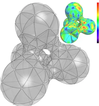
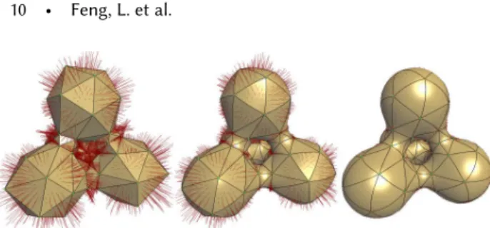
Fig. 1. Curved Optimal Delaunay Triangulations: A Bézier mesh (le�, here with cubic patches) can capture a curved domain with orders of mag-nitude less elements for a given Hausdor� distance. Our extension of ODT to curved meshes results in a well-behaved Jacobian field (top: sizing-scaled determinant, with a few front elements removed to expose the interior).

using high-order elements—and thus, high-order basis functions— involves inevitable computational overhead, the drastic reduction of the number of elements needed to capture the domain boundary and the internal physical �elds with a given accuracy lowers the total computational time appreciably compared to the linear case.

However, generating such a curved high order mesh for an arbi-trary domain is signi�cantly more di�cult than its straight-edge analog: �rst, many staples of meshing (such as Delaunay triangula-tions or quality measures of mesh elements) only apply to straight-edge meshes; moreover, the use of higher-order polynomials to approximate the shape of a domain renders the numerical task more complex as it increases the occurrence of local minima in the en-ergy landscape involved in the boundary �tting process and of local fold-overs of the polynomial map. As a result, most approaches for curved meshing limit themselves to deforming the boundary of a straight-edge mesh to improve the spatial matching of the bound-ary. However, this approach is limited and far from optimal as it largely relies on a good coarse linear mesh to start with, and leads to high deformation near the domain boundary, thus hampering subsequent numerical accuracy where it is sometimes most crucial (e.g., for boundary layers in �uid dynamics).

This paper extends the successful Optimal Delaunay Triangula-tion (ODT) approach for generating isotropic triangle and tetrahe-dron meshes [Alliez et al. 2005; Chen and Xu 2004] to now form Bézier meshes of arbitrary order. By exploiting the numerical proper-ties of the original ODT technique and introducing a novel boundary

treatment, we show that our approach, which we coined Curved Optimal Delaunay Triangulation, generates curved meshes robustly and quite e�ciently. The resulting meshes require far fewer ele-ments to represent geometry or to guarantee accurate numerical solutions than their linear (straight-edge) counterparts.

1.1 Previous Work

We begin our exposition with a brief review of graphics and compu-tational science e�orts towards linear and high-order meshing.

From linear meshes... High quality meshing in graphics typically seeks the generation of non-degenerate meshes that o�er good con-dition numbers for common discrete isotropic operators like the Laplacian [Cheng et al. 2012]. While Delaunay meshes with local re�nements [Shewchuk 1998] have been shown most e�cient at generating good isotropic simplicial meshes, variational approaches (that is, methods relying on energy minimization) can dramatically improve the quality of the resulting meshes. Most notably, the con-cept of Optimal Delaunay Triangulations (ODT) [Chen 2004; Chen and Xu 2004] anchored in functional approximation has garnered attention for providing what can be argued as the simplicial equiv-alent of Centroidal Voronoi Tessellations [Du et al. 1999; Liu et al. 2009]. Its implementation in 3D along with details on the sizing �eld computations and boundary handling was studied by Alliez et al. [2005], and a hybrid approach mixing Delaunay re�nement and ODT optimization was later introduced [Tournois et al. 2009] to accelerate convergence and improve results. Recent improvements include an alternative boundary treatment [Gao et al. 2012] and vari-ous numerical accelerations [Chen and Holst 2011; Chen et al. 2014]. Today, the isotropic meshes obtained via ODT optimization con-sistently outperform other approaches (based on advancing front, bubble packing, etc) in terms of element quality (dihedral angles, aspect ratio, etc) for a given vertex budget.

To high-order basis functions... While simplicial meshes can be used for linear basis functions in the context of Finite Element Analysis, they can also accommodate the use of higher order basis functions which have been in high demand for simulation in com-putational �uid dynamics (CFD) and solid mechanics. Increasing the polynomial degree of basis functions within each element (clas-sically referred to as p-re�nement [Babuska et al. 1981]) allows for increased accuracy and faster convergence, often at a fraction of the computational cost of simply re�ning the simplicial mesh (h-re�nement). Scalar �elds are no longer just de�ned through values at nodes: more degrees of freedom per elements are now available, depending on the choice of basis functions and their polynomial orders. The accuracy gains brought by higher order basis in tetra-hedral �nite-element simulation were demonstrated in graphics by, e.g., [Roth et al. 1998] and [Weber et al. 2011]. However, the accuracy of �nite element solutions is often strongly in�uenced by how well the geometry of the domain is approximated, which limits the applicability of straight-edge meshes in practice.

To high-order meshing. Coarse straight-edge meshes conform poorly to curved domain boundaries, impairing the correct numer-ical imposition of boundary conditions. Modern simulation tech-niques, in particular Isogeometric Analysis (IGA), de�ne the geome-try of the domain with the same high-order basis functions utilized

for their Finite Element computations; that is, they use “high-order meshes” in the sense that the geometric description of the domains is a manifold assembly of curved isoparametric elements that are each de�ned through a geometric mapping with respect to a canon-ical simplex. However, degree elevation can be numercanon-ically di�cult to handle near highly curved geometric boundaries: conforming to the shape of a boundary with piecewise higher order polynomi-als can easily create locally inverted mappings or severe distortion which precipitously decrease the accuracy of subsequent compu-tations. Some graphics applications (notably, [Mezger et al. 2008] and [Suwelack et al. 2013]) use higher order meshes just to o�er a coarse embedding of a �ne geometry and accelerate computations; in this case, the presence of large Jacobians near the boundary is not necessarily an important issue. In practice, though, generating high-order meshes is typically accomplished by �rst constructing a straight-edge mesh that is subsequently curved and often regular-ized in case of invalidity (non-injectivity) of the geometric mapping. Regularization is usually achieved either through smoothing or mor-phing [Karman et al. 2016; Ruiz-Girones et al. 2017] (the deformation on the boundary is propagated onto the inside of the domain), or through optimization of control points and topological changes to increase the smallest value of the local determinant of the Jacobian of the map [Cardoze et al. 2004; Luo et al. 2002]. Global mesh op-timization based on the extended notion of quality measures for curved elements has also been proposed: one can extend the element-based distortion measure by integrating a Jacobian-element-based distortion measure on the whole physical curved element [Gargallo-Peiró et al. 2013]. Distortion measures are often based on the Jacobian determi-nant, and include the ratio of minimum to maximum determinants in each element, or the ratio of the minimum determinant to the determinant of the corresponding straight-edge element [Johnen et al. 2013]. However, these functionals can be very high order even for moderately high order elements; Geuzaine et al. [2015] thus proposed a technique to compute provable bounds on the Jacobian determinant per element to check the mesh validity e�ciently, and formulated a simpler functional to untangle invalid parts with a log barrier to penalize small determinants. Hierarchical methods pro-ceed to curve edges �rst, then faces, then elements [Ziel et al. 2017] although behavior on complex 3D domains has not been demon-strated. Arguably, the most successful family of curved meshing methods rely on a mechanical analogy: these optimization-based methods use an initial straight-edge mesh as a reference domain and minimize a non-linear distortion using FEM between the reference domain and the parametric elements, thus e�ectively computing an elastostatic solution where the distortion they target de�nes a potential energy of deformation [Abgrall et al. 2012; Johnen et al. 2013]. However, the non-linearity of the potential is often an obsta-cle to �nding a good minimum, and starting from a straight-edge mesh of the domain unnecessarily adds distortion if this mesh is not of high quality. Note that this approach was actually used in graphics, in the context of simulation by [Bargteil and Cohen 2014]: the authors suggested to use a rest pose of an elasticity simulation to be the end result of a previous simulation with a straight-edge tetrahedral mesh. However, they used a linear elastic model for sim-ulation purposes, whereas high-quality meshing typically requires non-linear models [Johnen et al. 2013; Persson and Peraire 2009].

1.2 Contributions

In this paper, we revisit the ODT framework and extend it to provide both a better handling of the boundaries and new foundations for curved meshing. We show that the measure of element distortion underlying the ODT approach can be reexpressed as a particularly-simple potential energy whose minimization amounts to an equidis-tribution of the gradient of the deformation �eld, thus regularizing simultaneously the size and shape of all simplicial elements. After formulating a non-shrinking traction to favor uniform and isotropic elements at the boundary, we show that this interpretation of ODT applies nearly as is for curved meshes made of Bézier simplices. The resulting “Curved Optimal Delaunay Triangulations” provide coarse geometric descriptions of arbitrary 2D or 3D domains with a much improved �t to the domain boundary due to their piecewise polynomial nature, see Figs. 1 and 11. Moreover, our construction naturally promotes smoothness of the gradient of the induced geo-metric map inside and across elements, thus o�ering high-quality curved meshes ready to use in high-order �nite element methods.

2 REVISITING OPTIMAL DELAUNAY TRIANGULATION

Before describing our extension of ODT to high-order meshes, we �rst review the foundations behind ODT for straight-edge simplicial meshes in íd_{(d =2, 3). We show that they can be neatly rewritten in} the context of elastostatics, which provides us with a new approach to handle boundary conditions for improved isotropic simplicial meshing. This novel interpretation will, in later sections, render the extension to high-order meshes quite straightforward.

2.1 Primer on ODT

The quest for high quality simplicial meshes has sparked advances in mesh optimization through local vertex relocation to optimize a chosen notion of mesh quality [Amenta et al. 1999], local topological operations [Cheng et al. 2000], or both [Freitag and Ollivier-Gooch 1997]. Within the large body of work in mesh optimization for 2D and 3D unstructured triangulations, the Optimal Delaunay Tri-angulation approach (ODT for short) stands out by casting both geometric and topological mesh improvement as a single, uni�ed optimization [Chen and Xu 2004].

Approximation-theoretical foundations. Exploiting functional ap-proximation theory for piecewise linear interpolants, ODT �nds a simplicial mesh in dimension d that minimizes in Rd+1_{the volume} between the height �eld of the function f : x! kxk2_{and the} piece-wise linear (PWL) interpolation of the mesh vertices lifted onto the height �eld; that is, the mesh connectivity and vertex positions are updated so as to minimize the energy EODT:

EODT=k f fPWLk_L21=

π

fPWL(x) f (x) dx. (1)

The minimum of this energy is known to be asymptotically achieved when the mesh elements are isotropic [Nadler 1986]. Such theo-retical grounding has far reaching practical implications: optimal connectivity, seemingly a high dimensional combinatorial problem, results from a simple numerical minimization akin to a convex hull algorithm, for which many robust, o�-the-shelf tools exist. More-over, various closed-form expressions of this geometric de�nition have been proposed that allow to evaluate e�ciently the energy’s

gradient with respect to mesh vertices. In particular, if one denotes i as the one-ring neighborhood of vertex xi, we can rewrite the energy as a simple weighted sum plus a constant that solely depends on the shape of the domain [Chen and Xu 2004]:

EODT= 1 d +1 ’ i=1.. |V | kxik2| i| π kxk2dx. (2) A simple expression of the energy restricted to a single simplex was also formulated in [Chen and Holst 2011], containing no extra terms that depend on the domain:

EODT = | | (d + 1)(d + 2)

d+1_’ i, j=1,i <j

kxi xjk2, (3) meaning that the contribution of a simplex to EODTis proportional to its volume | | times the sum of all of its squared edge lengths.

Minimization of EODT. The minimization involved in �nding an

optimal ODT mesh in connectivity and vertex positions is particu-larly simple: starting from an arbitrary mesh of , one alternatively updates mesh connectivity for �xed positions, then vertex positions for a �xed connectivity [Alliez et al. 2005]. Vertex optimization in-volves minimizing a quadratic energy for inner vertices with respect to each vertex position, while connectivity optimization corresponds to �nding the Delaunay triangulation of the current vertex posi-tions, leading to a steady decrease of the energy after each iteration. The e�ect on the mesh is very visible: all elements quickly tend to become equally sized and equally shaped, as predicted by ap-proximation theory. Faster convergence can also be obtained using variants of Newton’s method, where the energy Hessian is approxi-mated through either previous values of the gradient [Chen et al. 2014] or a graph-Laplacian [Chen and Holst 2011].

Controlling mesh density. Another property of ODT making it particularly appropriate for isotropic meshing is that its formulation can be trivially altered to handle arbitrary mesh density: given a positive scalar �eld : ! R+_{, we can modulate the L}1_{norm in} the de�nition of EODTin Eq. (1) by substituting a modulated local

volume form (x) dx for the original dx as introduced in [Chen and Xu 2004] and exploited in [Chen et al. 2014]. Modifying the volume form does not a�ect the isotropic properties of formulation, but the resulting minimizer of the ODT energy now has elements with edges proportional to 1/(d+2)_{. A given sizing �eld h over the} domain can thus be imposed by picking (x) / h (d+2)_(x).

Non-shrinking boundary conditions. As oftentimes for variational problems, setting proper boundary conditions is crucial to the suc-cess of ODT: like Eq. (3) clearly indicates, minimizing EODTwithout

any constraints on the domain will make all the vertices of the mesh collapse to a point. Boundary conditions must thus be set to prevent shrinkage. Dirichlet conditions using a �xed sampling of the bound-ary of produces nicely-shaped tetrahedra throughout the domain, but generates many degenerate elements near @ (in particular, “slivers” in 3D, i.e., almost �at tets with nearly equal edge lengths) as boundary vertices are not optimized, preventing the formation of equilateral elements. Reprojecting boundary vertices [Alliez et al. 2005] or letting them slide along the boundary by only taking the tangential part of the ODT gradient [Chen and Holst 2011; Gao

et al. 2012] improves the resulting meshes, but leaves degenerate elements as vertices that reach the boundary tend to stay on the boundary. The work of [Tournois et al. 2009] exploits a degree of freedom in the boundary terms of the update of a vertex to enforce a “circumsphere property” on @ . This so-called Natural ODT bound-ary update guarantees that if ODT converges, it will form a mesh where boundary edges have nearly all the same lengths, further reducing the number of slivers. However, the precise boundary con-dition that this update corresponds to remains unclear, and as a consequence, how to modify this update to handle varying mesh density was not properly addressed either.

Discussion. While we will not explore anisotropy in this paper, we note that extensions of ODT to straight-edge anisotropic meshes have also been provided in [Chen and Xu 2004] and put into practice for �at and curved domains in [Boissonnat et al. 2006; Fu et al. 2014; Loseille and Alauzet 2009]. An interesting duality between graded polytopal tessellations and graded anisotropic simplicial complexes was also presented in [Budninskiy et al. 2016].

2.2 ODT as Elastostatics

We now reexpress the ODT energy in the context of continuum me-chanics. This physical analogy will help us de�ne a proper boundary condition (corresponding to a load on the boundary to render the elements isotropic there). This novel interpretation will facilitate the extension of ODT to high-order meshes later on as well.

Unit reference mesh. For any given d-dimensional simplicial com-plex T , one can de�ne a unit reference simplicial comcom-plex T where both T and T share the same connectivity, but each element of T is regular with all of its edges of length 1. Note that this reference mesh is trivially manifold, but cannot be embedded in d dimensions: except in the rare case of 2D triangulation with only valence-6 vertices, such a “unit” mesh can only be embedded in a Euclidean space of dimension D >d (and D is �nite due to Nash’s embedding theorem) since the generalized defect angles at vertices and edges are not zero. However, its exact embedding has no in�uence on our construction: this construction is only conceptual. Its purpose is to de�ne a clear intrinsic reference d-manifold so that our target “physical” mesh in Rd_{can be seen as a minimal deformation from} this ideal (but unrealizable in Rd_{) reference domain by a map as} in classical elastostatics, with:

RD T T ⇢ Rd

Our use of a reference domain with unit elements is quite di�erent from any of the other methods anchored in continuum mechanics such as [Abgrall et al. 2012; Bargteil and Cohen 2014; Johnen et al. 2013; Persson and Peraire 2009] as they all use non-unit straight-edge triangulations as reference, which unnecessarily biases the notion of isotropy based on the quality of the tetrahedron mesh they start from. Instead, our interpretation phrases the optimization as a minimization of distortion with respect to a perfect mesh.

Jacobian-based expression of ODT. For the original straight-edge case of ODT, the mapping is piecewise linear, mapping each unit simplex i from T to its associated physical simplex iin T . The Jacobian r of this map is thus piecewise constant: let’s denote Ji

this Jacobian from ito i. We now present a simple, but important lemma that re-expresses the contribution of an element to ODT.

L���� 2.1. Using the linear map between iand i, one has: EODT

i =

| i|

2(d + 2)det(Ji) kJikF2,

where kJik2F=trace (JiJt_i), and detis the determinant.

P����. The squared Frobenius norm kJik2Fof Jitimes the volume

of i is nothing but the integral of the Dirichlet energy of over i. From [Meyer et al. 2003; Pinkall and Polthier 1993], we know that the Dirichlet energy in 2D and 3D is a linear combination of squared edge lengths of i:

π i kr k2F = ’ i, j=1.. |V | ij kxi xjk2,

where the coe�cients ijdepend on geometric measures of i(half the cotangent of the tip angle in 2D [Pinkall and Polthier 1993], and one sixth of the cotangent of the dihedral angle times the associated edge length in 3D [Meyer et al. 2003]; more generally, they are the sti�ness matrix coe�cients for the Poisson problem). When iis a regular d-simplex, these coe�cients are all equal to 2/(d+1). More-over, we know that det(Ji)= |i|/| i| as the map is piecewise linear. We thus conclude that the expression of EODTrestricted to ias given in Eq. (3) is proportional to det(Ji) kJik2F, with a coe�cient of

pro-portionality equal to1₂| i|/(d +2) (for completeness, the volume of a d-dimensional unit and regular simplex is | _i| = (d+1)1/2/[2d/2d!]). Remark that this �nal expression is translation invariant (because of the gradient of ) and rotation invariant (kJkF2=kRJk2F for any

rotation matrix R), justifying a posteriori our claim that the precise embedding of the unit reference mesh does not matter. ⇤ ODT energy as potential energy. Based on the previous lemma, we directly deduce that the ODT energy can be seen as a potential energy density WODTover the reference con�guration T in the

context of hyperelasticity, expressed as:

WODT( J ) = _{2(d + 2)}1 det(J) kJk2F. (4)

With this expression, the potential energy of a given physical mesh is exactly equal to EODT. A potential energy density W induces an

internal (Cauchy) stress tensor over T of the form [Ogden 1997]: = 1

det(J) @W

@J · Jt. Since @kJk2

F/@J = 2 J and @ det(J)/@J = det(J) J t, we get a very

simple expression for the elementwise stress tensor in ODT: T������ 2.2. The Cauchy stress tensor ODTis expressed as:

ODT i = 1 d +2  JiJti +1_{2 kJ}ik2FId ,

whereId denotes the d ⇥ d identity matrix.

As a consequence, an optimal ODT mesh satis�es div( ODT)=0

everywhere (in the weak sense of FEM), as it is the equilibrium equation for the equivalent elastostatics problem we just proved.

Fig. 2. Non-shrinking ODT. Starting from a random triangulation (top: 2D; bo�om: 3D), minimizing the ODT energy with our non-shrinking boundary loads naturally converges (le� to right) to a mesh with isotropic elements.

Connectivity of unit reference mesh. Since we showed that the ODT energy is in fact the integral of a potential energy density, we can also immediately conclude that the minimal potential energy for a given set of vertex positions is attained for the unit reference mesh that corresponds to the connectivity of the Delaunay triangulation of the vertices in physical space. As the reference mesh is purely conceptual, no computations besides �nding the Delaunay triangu-lation is required: it simply means that our elastostatics problem consists in �nding both the connectivity of the reference con�gu-ration and the deformed physical mesh that minimizes the total potential energy of the deformation, for given boundary constraints based on the domain . We will formally write this variational principle after we discuss boundary conditions.

2.3 Non-shrinking boundary conditions

Dealing properly with boundaries is key to the success of ODT. Our elastostatics rewriting of the ODT energy suggests using boundary forces, or loads, to prevent the degeneracy of the minimization. The simplest constraint is to add a boundary force density along the boundary equal to ODTn; in this case, boundary terms will exactly

compensate for the forces induced by the internal stress, prevent-ing the boundary vertices from movprevent-ing: this choice corresponds to Dirichlet boundary conditions. As previously discussed, such a treat-ment is not quite useful in our case: we wish instead to let vertices move around to generate boundary elements that are as isotropic as possible. This leads us to propose another expression: we can compensate the isotropic part of the ODT stress tensor only, thus leaving the deviatoric part (containing shearing forces) active near the boundary: with the corresponding boundary forces, the elasto-statics problem will �nd a solution where stress at the boundary is purely isotropic, i.e, elements are under equal compression/tension in all directions. Thus, at equilibrium, boundary elements will be isotropic. In order to impose such a traction, we directly apply the following boundary force �eld fbdryon a boundary element iin T (with the outwards unit normal denoted n):

fbdry= 1

d trace( ODT) n = 1

2d kJik2F n, (5)

since the isotropic part of is trace( ) Id/d and trace(Id) =d. As Fig. 2 demonstrates, this simple boundary condition added within the geometry updates unfolds a very uneven mesh into an assembly of perfect equilateral simplices, quickly and in a stable manner.

2.4 Discussion

Revisiting the original ODT energy through elastostatics provides some key advantages, as we review brie�y to conclude this section.

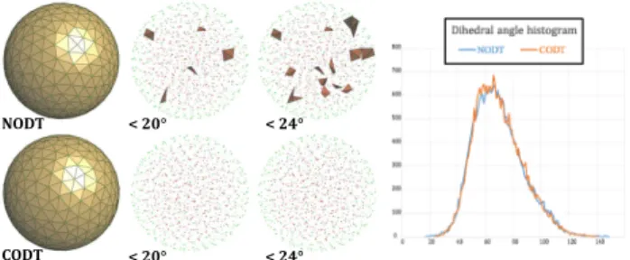
Fig. 3. Slivers. Given a spherical domain and 1,000 vertices, Natural ODT [Tournois et al. 2009] (top) achieves a minimum dihedral angle of 17.25 and a maximum of 149 , with 5 tets with angles below 20 (top); our new isotropic-stress boundary treatment (bo�om) brings the minimum angle to 24.75 and the maximum to 141 instead.

Variational formulation. First, we can now formulate the exact elastostatics problem that our modi�ed ODT solves:

(T⇤, ⇤)=arg min T, π TWODT(r (x)) dx s.t. 8>>< >> : @T= 1 2d kr k2FId Dist⇥ (T ), ⇤ , where Dist[·, ·] measures how far two subsets of Rd_{are from each} other. In practice, this last condition can be enforced by adding a boundary �tting force �eld that attracts boundary elements of T towards @ . Such a force can be derived from, e.g., the symmetric Hausdor� distance between mesh boundary and domain boundary, or simply from the volume in between the two [Alliez et al. 1999]. This attractive force �eld then acts as a penalty to enforce a close match between @T and @ , thus enforcing the last constraint. We will provide a simpler shortest-distance based force �eld in Sec. 3.5 when we treat the more general case of Bézier meshes. Our novel treatment of boundary elements brings much added robustness to the ODT procedure : the constant reprojection on @ used in Natu-ral ODT slows down convergence, introducing constant jittering of boundary vertices; in sharp contrast, the CODT treatment of bound-aries does converge reliably in practice, always reaching a high quality mesh. Even if we compare to the (non-converged) best result of natural ODT after many iterations, our new approach converges to a lower number of slivers as illustrated in Fig. 3.

Interpretation and other potential energies. A posteriori, expressing ODT as a minimization of the deformation of a map between an ideally isotropic mesh and the current embedding of a mesh in Rd raises the question of why this particular choice of potential energy is special. We �rst note that the potential energy that ODT corresponds to is a local rescaling of the usual Dirichlet energy density: without the volume | | in Eq. (3), we would be left with only the Dirichlet energy, enforcing conformality of the map but not size uniformity. Moreover, one could also argue that using a geometric energy density of the form min_R2SO(d)kJ RkF2in the

spirit of what is advocated in [Chao et al. 2010] for elastic simulation would seem like a perfect substitute: it would force each element to be isometric (up to a global scale ) to its reference element. In fact, the potential energies of [Johnen et al. 2013; Persson and Peraire 2009] (or more generally, any energy that derives from shape functionals through density integration [Gargallo-Peiró et al. 2013])

target the same ideal: having a Jacobian as close to constant and isotropic as possible. However, two important di�erences make these other choices of energy less attractive. First, �nding the optimal connectivity of these energies for given positions of the physical mesh nodes is not known, which will thus require local and costly exploration of the huge combinatorial space of all connectivities; instead, the ODT energy is known to be minimized for a Delaunay connectivity [Chen and Xu 2004], which is e�ciently computed by a number of existing libraries. Second, solving for the optimal position of vertices given a �xed connectivity requires a non-linear solve, and the minimization of high-order energies is evidently slower and more prone to local extrema than ODT, for which the optimal positions are found through a sparse linear system. One can thus consider ODT as the d-D continuum equivalent of 1-D zero-rest-length springs that regularize simultaneously the size and shape of all simplices: the ODT energy goes to zero when the volume of simplex goes to zero, whereas previous elastic energies had a non-zero volume at rest state. In fact, the ODT energy is nothing but the (integrated) L2norm of the Jacobian over the physical domain, so its minimization will tend to equidistribute its singular values. This simple energy is thus a more e�ective solution to target a uniform, isotropic Jacobian �eld than springs with unit rest lengths, as they would require non-linear solves. Note also that other quality measures [Knupp 2001; Shewchuk 2002] could be used as substitute potential energies to enforce good mesh elements, but none can be simpler (i.e., lower order in vertex positions) than ODT.

3 CURVED OPTIMAL DELAUNAY TRIANGULATION

We are ready to delve into our extension of ODT for high-order meshes. We focus on Bézier meshes in dimensiond (ford =2 ord =3), made out of Bézier simplices of order n. This choice of parametric elements has commonly been used in graphics, as they require fewer points (thus less memory) to represent curved domains and have much better continuity properties than linear elements.

3.1 Primer on Bézier Meshes

While meshes made out of Bézier simplices (sometimes referred to as Bernstein-Bézier meshes) have often been used in the graphics literature (see, e.g., [Bargteil and Cohen 2014; DeRose 1988; Roth et al. 1998; Weber et al. 2011]), we brie�y review their construction here for completeness.

Preamble. In the previous section, we used a linear map between a regular simplex and an arbitrary simplex embedded in íd_{. With} this convention, a straight-edge simplex is actually a parametric patch, where the parameter domain

is the regular simplex, and the inter-polation between the vertices of the physical simplex is through linear ba-sis functions. The Jacobian of this geo-metric map (which is constant per

simplex since the basis functions are linear) indicates the local devi-ation between the canonical and the physical element, and the ODT energy tries to render this Jacobian �eld as uniform and isotropic as possible. Bézier simplices extend this geometric map notion to now higher-order polynomial deformation functions, where vertices

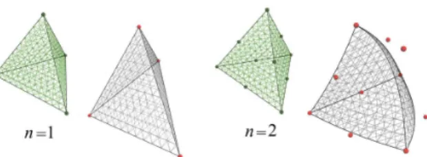
Fig. 4. Bézier simplices: Examples of Bézier simplices for n =1 (le�, sim-plicial meshes) and n = 2 (right, quadratic patches), with control points highlighted in red; top: their reference (straight-edge) regular simplex.

are enriched with other control points per simplex to increase the space of possible deformations.

Barycentric Coordinates. The use of barycentric coordinates is particularly convenient when dealing with simplices: any point x in a simplex in íd _{is encoded by a column vector of (d +1)} non-negative coe�cients u(x) B (u1,...,u_d+1)t, which sum to one. We denote by U the matrix of the di�erential of the linear map from x to u (i.e., the Jacobian matrix); it is constant over the simplex since barycentric coordinates are linear. Given that we only consider regular simplices , its expression is the same for each simplex, and is given in App. B for 2D and 3D.

Bernstein polynomials. A barycentric indexi of order n is de�ned by a vector of (d+1) non-negative integers i = (i1,...,i_d+1) 2 éd+1 that sum to n, i.e., |i| BÕkik=n. For each such index corresponds a Bernstein polynomial Bn

i over the simplex (the superscript n refers to the order of the subscript i), de�ned through:

Bn_i(u) =Œd+1n! k=1ik! d+1 ÷ k=1 uik k, (6)

where u is a shorthand for u(x). These polynomials have a num-ber of interesting mathematical properties (e.g., partition of unity, positiveness over the simplex), not the least being that their partial derivatives are, themselves, scaled Bernstein polynomials:

@

@u_kBni(u) = nBn 1i ek(u) (7)

where ekdenotes the vector of size (d+1) with 1 at the kth position and all zeros otherwise (to be valid for any n, Bernstein polynomials are assumed to be identically zero if one of the barycentric indices is negative). Note that we will denote by Bn

i the Jacobian (row vector) of Bn

i with respect to the barycentric coordinates, i.e., Bin(u) = h _@ @u1Bni(u) · · · @ @ud+1B n i(u) i (8) Eq. (7) = nhBn 1_{i e1}(u) · · · Bn 1_{i e} d+1(u) i .

Bézier simplex. We now can properly de�ne a d-dimensional Bézier simplex of order n: given a set C of control points with

C= {ci2 íd| i 2 éd+1,|i| = n},

the associated Bézier simplex is de�ned via its geometric map : x = (x) B ’

|i|=n

ciBni(u(x)). (9) The control points ci2 ídare degrees of freedom for the Bézier simplex, allowing it to curve. Note, as mentioned earlier, that the case n =1 is nothing but the piecewise-linear map described in Sec. 2

since the Bernstein polynomials are linear, and the control points are restricted to be the vertices of the linear mesh. More generally, a Bézier simplex only interpolates its “corner” control points (i.e., those of the form cn_ek), whereas the other control points smoothly

pull and stretch the simplex towards them, see Fig. 4. Note also that this construction has the property that the boundary of a Bézier k-simplex is, itself, a Bézier (k 1)-simplex.

Map Jacobian. Knowing the Jacobian U of u w.r.t x and the Jaco-bian Bn

i of the Bézier simplex w.r.t. u, we can directly express the Jacobian of the geometric map of the Bézier simplex w.r.t. x as:

J(x) B r (x) =✓ ’ |i|=n

ci· B_in u(x) ◆

U(x) (10) We deduce directly that the change @J(x)/@ciof the Jacobian with respect to a control point ciis given by:

@J(x) @ci =B

n

i u(x) U(x). (11) Bézier mesh. A Bézier mesh is a manifold assembly of Bézier simplices, that is, any two adjacent Bézier simplices have their as-sociated parametric regular k-simplices sharing a common (k 1)-simplex for k  d. Moreover, two adjacent k-simplices share the same (locations of) control points on their shared (k 1)-simplex as well, thus enforcing continuity across simplices. Note that the expression of the Jacobian with respect to a control point ciderived for a single element in Eq. (11) remains valid as is, but one has to sum the contributions of each simplex sharing this control point if needed to get the �nal Jacobian.

Cubature points and cubature samples. For a function (u) de�ned in barycentric coordinates over a d-simplex, its integral over the Bézier parametric simplex can be evaluated numerically using a cubature scheme. For this purpose, we de�ne a set of weighted points {(ui,wi)}iover the reference simplex such that Õiwi=1: they de�ne a cubature scheme with which a function can be integrated through a linear combination of sample values as_π

(u) ⇡ | |’ j

w_j (uj) .

Additionally, we map these cubature points to the physical domain to create a series of cubature samples {xjB x(uj)}jfor each Bézier simplex. This sampling of the Bézier simplices will be useful when dealing with boundary �tting: they provide an e�cient way to eval-uate surface integrals by only using values at these spatial samples.

3.2 Extending ODT to High-Order Elements

Straight-edge triangulations correspond to Bézier meshes of order one, so one may be tempted to extend the approximation theory foundations behind ODT to the general case of order n. However, the best discrete approximant of the paraboloid is no longer relevant here: any Bézier simplex of order more than one can exactly capture this low-order polynomial height �eld. Using a higher-order polyno-mial to replace the paraboloid is also bound to fail, as one loses the convenient property that the function and its discrete approximant are below one another, rendering the L1norm di�cult to evaluate.

However, our analogy with continuum mechanics still holds in the high-order case. We proved in Lemma 2.1 that the ODT energy

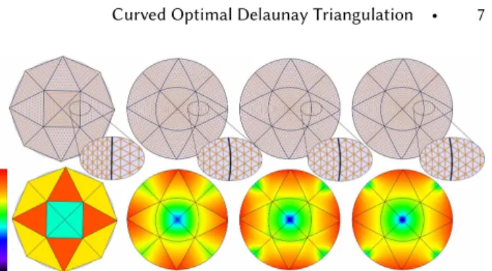
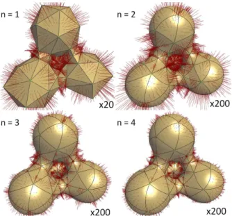
Fig. 5. Determinant of Jacobian. From le� to right: ODT mesh (n = 1), then curved ODT meshes with order 2, 3 and 5 respectively, showing in-creasing continuity across elements. Bo�om: determinant of the Jacobian in the domain visualized with a rainbow colormap.

of a mesh corresponds to a speci�c potential energy of the piece-wise linear map between an idealized unit reference mesh of same connectivity and this mesh. Since each element of a Bézier mesh has a simplicial parametric domain and the map is now piecewise polynomial, the exact same expression is well de�ned in this Bézier context. We rename it ECODTto underline its validity on any Bézier

mesh of order n 1:

De�nition 3.1. Given a Bézier mesh T made out of d-simplices of order n and its unit reference mesh T made out of its associated equilateral simplicial charts with the same connectivity, we de�ne its Curved Optimal Delaunay Triangulation energy as:

ECODT=_{2(d + 2)}1

π

Tdet(J(x)) k J(x)k 2

Fdx, (12)

where J(x) is the Jacobian of the Bézier simplex at point x on the parametric domain.

Polynomial degree of ECODT. For Bézier simplices, this energy is in

fact polynomial in the barycentric coordinates. In a Bézier d-simplex of order n, the Jacobian has degree n 1, and its determinant has degree d (n 1). Thus, the energy density is of polynomial degree (d+2)(n 1). In practice, order-2 (resp., order-3) Bézier elements in 2D and 3D are often used, leading to polynomial degrees 4 and 5 (resp., 8 and 10). Note that more complex energy densities (as discussed in Sec. 2.4) would raise the degree of this polynomial, or even render the energy rational, adding signi�cant di�culty to its evaluation and, arguably more troublesome, its minimization.

Interpretation for higher-order meshing. While the ODT energy is clearly promoting equilateral simplices, a closer look is needed to understand the e�ect of a low CODT energy. In the case of a piecewise linear map , the energy in a simplex was proportional to its volume and to the squared Frobenius norm of Jacobian describing its linear transformation from a regular simplex, see Lemma 2.1. In a Bézier simplex, the reference (parametric) element is still a straight-edge simplex, so the notion of unit reference mesh remains valid and unchanged. But now, the actual elements are curved, so the traditional notion of “well-shaped elements” in simplicial meshing is no longer appropriate. However, what this energy does is, in essence, to consider the Bézier mesh subdivided to an in�nitely dense mesh, where now the edges are nearly straight, and it sums up the classical ODT energy for these �ne sub-simplices. So minimizing

Fig. 6. Man head. Order-3 Bézier meshes based on a sizing field derived from the local feature size with 1K vertices (le�, no sliver peeling) vs. 10K vertices (right); the sizing-scaled Jacobian determinant is visualized (bo�om) via a rainbow colormap; respective closeups on the ear and nose (middle).

this energy will lead, instead, to a Jacobian �eld of the deformation map between the Bézier parametric domain and its curved elements as close to being uniform and isotropic throughout the domain. This e�ect can be clearly noticed in Fig. 5: starting from an ODT mesh, optimizing the control points of a Bézier mesh to minimize the energy ECODTmakes the local Jacobian �eld more continuous

across edges—not to mention that the same number of elements now approximates the smooth domain much better (see also in Fig. 11 how the Hausdor� distance to the boundary quickly decreases with

order). This continuity of the Jacobian �eld will improve within, and across, elements as we go higher in the order of the Bézier simplices, but not necessarily at vertices that form a cone singularity in the reference domain: Fig 5 shows this expected behavior by displaying the determinant of the Jacobian for a high-order Bézier mesh, which is smooth everywhere except at vertices with irregular valences.

Derivative of CODT energy. The derivative of CODT energy de-�ned in Def. 3.1 with respect to a Bézier control point ciis found by the product rule (see App. A for the full derivation), leading to:

@ECODT @ci = 1 2(d+2) π TB n i(u(x))U(x)⇥k Jk2FJ1+2Jt⇤det(J)dx. (13)

3.3 Bézier mesh topology

We also need to consider the topology of the Bézier mesh, in partic-ular to �nd how to optimize the connectivity based on the CODT energy, and which elements are inside the domain.

Proxy straight-edge simplices. As often used for Bézier meshes, we �rst de�ne the notion of “proxy simplex” for a Bézier simplex to be the straight-edge simplex formed by the vertices (i.e., corner control points) of the Bézier patch (inset: order-5 simplex, proxy in blue). For n =1, this is exactly the Bézier simplex; for higher

orders, it is just a straight-edge approximation of the curved element. Delaunay proxy connectivity. Remember that for the straight-edge case, the minimum of the EODTfor �xed vertex positions is achieved

for the Delaunay connectivity of these positions. With this new, extended CODT energy, the situation becomes more complex: now, the position of the control points do depend on this connectivity, so �nding which connectivity minimizes the CODT energy is less obvious. We are not aware of how to de�ne the optimal connectivity of the Bézier mesh; however, since we are trying to form a Bézier mesh with a distortion as small and uniform as possible, we pro-ceed with the following assumption: we simply enforce a Delaunay connectivity for the proxy elements. That is, from the vertices of the Bézier mesh only (disregarding the other control points), we com-pute the Delaunay triangulation of these positions, and assume that the resulting Bézier mesh with these Delaunay simplices as proxy elements is the one with minimal energy.

Restriction to . Given a set of ver-tices and a Delaunay connectivity for the proxy elements, we have formed a Bézier mesh. However, not all of the elements are relevant to the meshing of the domain. In particular, concave regions may con-tain Bézier simplices that should really be considered as outside, and thus

dis-regarded when it comes to optimizing the meshing of . For a Delaunay (straight-edge) �rst-order Bézier mesh, there is a clear way to identify elements inside through the notion of restricted Delaunay elements [Rineau and Yvinec 2008]: these are simplices for which their Voronoi dual is inside . Only those restricted mesh elements are active during ODT optimization, as they correspond to the set of inside elements. We thus proceed exactly the same way

for our case, but by testing the proxy elements instead: every Bézier simplex whose proxy element is restricted is tagged as active. A �ner approximation could be done by considering the subdivided control net; but only testing the proxy elements has shown su�cient in all our examples.

Finally, we also deactivate restricted boundary elements that have two faces or more on the domain boundary and are not on a sharp feature: this allows to quickly “peel o�” sliver-like curved elements. Such curved slivers can be useful if only a concise representation of the domain is sought after, but they are not acceptable for �nite element computations as they lead to singularities of det J. Fig. 7 depicts such an example in 2D and Fig. 16 (bottom) in 3D, each involving a simplex angle close to 180 degrees.

Fig. 7. Singularities at obtuse angles. If a curved triangle loosely approx-imates a disk in 2D (le�; proxy triangle in blue), the Jacobian is well behaved everywhere. For strong fi�ing forces (middle), near-zero Jacobians may oc-cur at vertices when the angles become close to 180 degrees, see the dark magenta color and the squeezed subtriangles in the two insets (right).

Boundary elements. Our identi�cation of restricted elements also provides a direct way to �nd which Bézier faces are on the external boundary of our Bézier mesh: during the testing of restricted ele-ments, any d-dimensional simplex for which one of its (d 1)-faces’ dual edges crosses @ is tagged as “boundary simplex”, and the corresponding boundary face is tagged as “boundary”: they will play an important role in �tting the domain.

3.4 Non-shrinking boundary conditions

As we discussed in Sec. 2.1, de�ning proper boundary handling is important to obtain meshes with low shape distortion. While previ-ous boundary conditions do not always carry over straightforwardly to our curved meshing context, our new isotropic-stress boundary condition discussed in Sec. 2.3 can be adapted rather easily.

At �rst, one may be tempted to simply apply a force fbdry(given in Eq. (5)) pointwise along boundary elements, since the gradient J of the map is now spatially varying. This is, however, forgetting part of the goal of this boundary force. Remember that the internal CODT energy tries to get the Jacobian as uniform and isotropic as possible. But the boundary condition should also promote both isotropy and uniformity of the Jacobian.

We thus propose to compute an average tensor per boundary simplex, and apply this tensor to form the boundary traction. More

speci�cally, we compute the average hkJk2Fii (over area in 2D, over

volume in 3D) of the isotropic part of the CODT stress tensor of a boundary simplex. Then we apply the following boundary force �eld for the face(s) of ithat are tagged as “boundary”:

fbdry= _{2d hkJk}1 F2iin.

This averaging of the isotropic part of the stress at the boundary used as an element-wise traction now promotes both isotropy and uniformity: equilibrium will be reached when the Jacobian is, on average, isotropic and uniform. It also exactly �ts the straight-edge ODT case, as the average and the pointwise Jacobian are equal in the piecewise linear map case.

3.5 Boundary fi�ing

Minimizing our CODT energy with added traction at the boundary makes any Bézier mesh as “regular” as possible in the sense that it has a Jacobian with respect to the parametric domain quite uniform and isotropic: in fact, like in Fig. 2, running the usual control-points / proxy-connectivity procedure to minimize the CODT energy leads to nearly linear elements, as these correspond to the best possible element in terms of their Jacobian �elds. Yet, the domain may not be particularly well approximated by restricted elements, unless the mesh is very dense. One of the key advantages of Bézier meshes is that they can adapt to curved domains with high precision even for a small count of elements thanks to the added �exibility a�orded by the control points and high order basis functions.

In order to achieve this desirable property, we add a boundary �tting force �eld on the boundary faces of T to push them towards the boundary @ of the domain. The magnitude of this extra force o�ers a compromise between boundary �tting and low distortion of the Bézier map. Depending on the application for which a mesh is constructed, vertices may have to be precisely on the boundary, or the mesh boundary just needs to approximate @ . While the former can be achieved using methods as in [Alliez et al. 2005; Chen et al. 2014; Gao et al. 2012], we derive a simple approach to the latter by exploiting the stability of our non-shrinking minimization.

We simply add a boundary force �eld f�tthat attracts the bound-ary face elements of T to the domain boundbound-ary @ using a two-sided notion of distance minimization. For any cubature sample xi of a d-simplex that is on @T , we apply a local �tting force that sums a force �eld fT! based on the shortest distances from T to and

another force �eld f !Tbased on the shortest distances from to

T to ensure tight geometric closeness:

f�t(xi) = | |1/d fT! (xi) + f !T(xi) , (14)

where | | is the volume of the d-simplex on which point xilies, and is the global strength of the force. The �rst force is de�ned as:

fT! (xi) = @ (xi) xi,

where (xi) is the projection of xi to the nearest point on the domain boundary @ . The vector @ (x) x is known to be the local gradient of the one-sided squared distance function between @T and @ [Pottmann and Hofer 2003]. By applying this force to all cubature samples (weighted by their associated areas), we obtain a simple one-sided boundary �tting term whose integral is zero when the boundary of the Bézier mesh is straddling the domain

Fig. 8. Fi�ing force field. The fi�ing force field decreases in magnitude as the mesh of Fig. 1 (n = 3) is optimized from a very coarse linear mesh. Force vectors are scaled by a factor 20 for be�er visual depiction.

boundary. The use of this force alone is usually enough to attract the Bézier mesh to the boundary of the domain, but its one-sidedness may lead to regions of the domain boundary being not covered. So we compute the force f !Tderived from a set of sample points

{sk}ksampling the boundary @ : for each boundary sample sk, we compute their closest cubature sample xion the boundary @T of the Bézier mesh; we then add a force f !Tequal to the vector between

the cubature sample and the centroid of all closest boundary sample points, restricted to be normal to the boundary (to prevent spurious sliding due to the use of the centroid):

f !T= 1 |S(xi)| ’ k 2S(xi) sk xi ! · nini, (15) where S(xi) is the set of boundary sample indices such that xi is their closest cubature sample, and ni is the unit normal to the Bézier surface at xi. This extra forcing term helps ensure that every region of @ is close to the Bézier mesh. The resulting force is further multiplied in Eq. (14) by the local edge length h (obtained by taking the d-th root of the volume of ) and a dimensionless coe�cient for two reasons: �rst, it makes the �tting force be of the same dimensionality as the gradient of CODT, thus making these forces comparable in strength locally; second, the value can be interpreted as controlling h/ where is the average distance of the boundary face of ito the boundary of . That is, is a scale-invariant parameter de�ning how close to the boundary we want the mesh to be compared to its local element size. This coe�cient is thus easy to adjust based on the balance between mesh distortion and boundary �t, independent of mesh density or domain shape. Refer to Fig. 9 to see the e�ect of increasing values of .

3.6 Mesh gradation

For a sizing �eld h(x) over , all the expressions we provided need to be altered to lead to the requested sizing constraints. Most changes are very simple, and are best understood as thinking of sizing as a modulation of the local metric by 1/h. This means that any gradient needs to account for h (for instance, the evaluation of J should become J/h), and any local evaluation of length, area, or volume in should be multiplied by h 1, h 2or h 3respectively. As a result, the ODT energy is e�ectively multiplied by h (d+2)_{pointwise as} mentioned in the straight-edge case, since it involves kJk2

F(bringing

a factor h 2_{) and det(J) (responsible for a factor h} d_{). The only} complication is the computation of the derivative of the sizing-weighted CODT energy, as it now involves a derivative in the sizing

Fig. 9. Boundary fi�ing. The dimensionless fi�ing strength in Eq. (15) controls the tightness of the fit to the domain boundary: a small value (le�, =1) will only weakly capture the boundary shape, while a large value (right, =100) provides a close fit. The e�ect is adapted to the size of local elements, making its value scale invariant, thus intuitive and easy to set.

�eld itself; for completeness, we provide its derivation in App. A and its complete expression to ease implementation in Eq. (23).

As reported in prior work, we found that having a slowly-varying sizing �eld that is adapted to the local feature size (lfs) of the domain (see, for instance, the lfs-based K-Lipschitz �eld in [Alliez et al. 2005]) is best for the gradation of the resulting mesh, as well as for the robustness of the meshing process as the size of elements �ts the local geometry well. See Fig. 10 to see the e�ect of varying mesh densities for a given domain, using degree-3 elements.

Fig. 10. Sizing. Le�: uniform sizing; middle: lfs-based sizing; right: radially linear sizing function. Respective sizing fields h are depicted on top.

3.7 Pu�ing it all together

While minimizing the CODT energy can be incorporated into any meshing technique with minimal e�ort, we describe next how one can construct an isotropic curved Bézier mesh from an input domain and a sizing �eld h (possibly constant for uniform meshes). In particular, we mention a few important implementation details to improve e�ciency and robustness.

Mesh initialization. Starting from a decent mesh is preferable if computational time is an important issue—but any mesh can do. In practice, we initialize the vertices by drawing them randomly from a density distribution adapted to the sizing �eld. Our implementation follows a usual Delaunay re�nement/deletion process [Cheng et al. 2012; Rineau and Yvinec 2008] to construct a restricted tetrahedron mesh that roughly follows the sizing �eld h and captures the topol-ogy of the domain . This coarse mesh de�nes proxy elements from which a �rst Bézier mesh can be initiated.

Fig. 11. Boundary approximation. Input domain approximated for a given number of vertices, from Bézier order 1 to 4. The respective 2-sided Hausdor� errors (as a percentage of bounding box diagonal) are 3.42, 0.315, 0.133 and 0.073. The boundary forces are rescaled for be�er depiction.

Numerical integration using cubature. Since the Bézier mapping we employ is polynomial and the CODT energy is a function of its Jacobian, the integrals involved in our CODT energy and its deriva-tive can be evaluated e�ciently and exactly using a cubature scheme with the proper order (and with a pre-evaluation of the Bernstein polynomials of the cubature points for e�ciency) as their pointwise values are known in analytical form. Unless a constant sizing �eld is chosen, we use Witherden-Vincent cubature points [Witherden and Vincent 2015]: the presence of an arbitrary (i.e., non-polynomial) sizing �eld h is robusly handled through this cubature scheme—with, again, pre-evaluation of the �eld at the cubature points—because its weights are all positive. In our code, we used the points and weights of this cubature scheme provided in [Schlömer 2018].

Optimization of ECODT. From a current Bézier mesh, we perform multiple “rounds” of optimization of the CODT energy, i.e., alternate steps of geometry and topology updates to improve the mesh:

• Geometry. Control points (including vertices) are moved through quasi-Newton (more precisely, LBFGS) iterations, where we add to the gradient of ECODT(Eq. 11) the contribution of the boundary forces f�tand fbdryto the control points. More precisely, for each control point ci, we add to @J/@cithe boundary force for each cubature sample xkof neighboring simplices weighted by the value Bn

i(uk) of the Bernstein polynomial Bni for that cubature point uk. Since Bernstein polynomials form a partition of unity over each simplex, forces are properly distributed to the control points; the resulting vector forms the gradient (righthand side) of the quasi-Newton step, while the Hessian is approximated from previous gradients (we use a history size of 5 in our code). • Topology. Every 10 geometry updates, we verify that every proxy

element is still Delaunay, performing a topology update if needed.

Once a connectivity update is triggered, we make sure not to alter the control points of the una�ected elements; newly-created elements are assigned either existing control points for shared faces, or canonical internal control points as if they were forming a straight-edge simplex: these new control points will move at the next round of energy minimization anyway. To accelerate computations, this topology check is only done every 30 geom-etry updates once the energy change per iteration goes below a certain threshold: this indicates near convergence, and thus a low probability of frequent connectivity changes.

Early on, Jacobians with negative determinants may appear tem-porarily, corresponding to local foldovers in a Bézier patch. While minimizing the CODT energy eventually removes these cases, we found bene�cial to replace the determinant det of J by:

det < 0? 100 det: det.

This simple trick heavily penalizes any locally negative Jacobian by arti�cially in�ating its e�ect. Even with large �tting forces, our resulting meshes never have Jacobians with negative determinants. Boundary �tting. The boundary forces are directly used as a change of the gradient for the quasi-Newton step in each geometry update. Faster convergence is observed if we start with a small �t-ting force magnitude : we start with = 1 and increase gradually during the geometry updates of the Bézier mesh to reach = 1000. With this scheduling (see Fig. 14 for an example), mesh elements have time to quickly position themselves near the boundary and equidistribute their Jacobian before the �tting force is too strong and starts counteracting the e�ect of the CODT minimization.

Sharp features. With the algorithm de-scribed above, sharp features and corners may or may not be properly handled, as shown in the inset (where depending on the initialization, the features get exactly captured (left), or at times, an element is bent to only approximate the feature (right)). Sharp features can, however, be tackled properly if needed. Recall that the

mesh boundary corresponds to facets of “restricted” proxies. Instead of having only �tting forces between the mesh boundary and the domain boundary, we can put �tting forces between all domain features and restricted Delaunay elements (facets, edges, vertices). More generally, restricted Delaunay elements are elements whose dual intersects the corresponding feature in the domain. For 3D meshing, this includes all features of lower dimension (2D, 1D, 0D): the dual of a restricted facet (a Voronoi edge) pokes the domain 2D boundary as we used before; but now, an edge is restricted if its dual (a Voronoi face bisecting this edge) contains a sharp crease of the domain; and a vertex is restricted if its dual (Voronoi cell) contains a sharp corner. In practice, we thus sample all existing features. During optimization, we detect all these restricted elements within the proxy mesh after each connectivity update, and we call a Bézier element restricted if its proxy element is restricted. Before each quasi-Newton iteration, we calculate cubature points on all these restricted Bézier elements, then for each kind of features, we �nd the two-sided projection vectors between Bézier cubatures and domain

Fig. 12. Sharp features. With simple changes, our approach can accom-modate sharp features, ensuring that the curved edges of the Bézier mesh approximate the feature curves, while corners are at vertices. Restricted Bézier edges and vertices (i.e., creases and corners) are shown in red.

samples, just like f!Tand fT! in Sec. 3.5. The only di�erence with

Eq. 14 is the rescaling factor: to keep dimensionless, we use e2 and s3for edges and vertices respectively, where e is the local edge length and s is the average length of edges incident to the vertex. Three meshes with sharp features are shown in Fig. 12.

Interleaving re�nement/deletion/teleportations. Note that most of the previous accelerations proposed in the context of straight-edge ODT meshes can also be incorporated in the curved mesh extension. In particular, we found that the strategy of Tournois et al. [2009] consisting in triggering occasional re�nements (resp., deletions) of elements in regions where the determinant of the Jacobian is smallest (resp., largest) helps converge faster. The use of vertex teleportation recommended in [Alliez et al. 2005] achieves a similar goal, where now insertion and deletion are done in pairs.

Degree elevation. As recommended in previous works, proceed-ing through incremental degree elevation helps both accelerate convergence and improve the �nal mesh quality: even if CODT is signi�cantly simpler than previous mesh-optimization functionals, starting from lower order polynomials avoids stepping early into local minima, and minimize the amount of transient wiggling that high order polynomials are known to create. The use of lower-order numerical integration with fewer cubature points also improves e�ciency in early stages of the meshing.

3.8 Discussion

Our extension to ODT allows the creation of curved meshes with excellent properties, akin to the isotropy of ODT meshes. We review next a few notable properties that end users may bene�t from, as well as further possible extensions.

Isogeometric Analysis. In computational science, recent years have seen a growing interest in Isogeometric Analysis (IGA): the geom-etry of the computational domain is de�ned through parametric functions that are also used to approximate the unknown physical �elds in a numerical simulation. Such approaches avoid the typical mismatch between the basis functions describing the geometry and the ones de�ning the solution space in the domain, thus improving the analysis and convergence of numerical methods. Our curved extension of ODT may be particularly relevant to this community:

because we optimize the parameterization to ensure a high quality map gradient within and across elements, IGA-based numerical sim-ulations should have both improved condition numbers of sti�ness matrices and global accuracy [Pilgerstorfer and Jüttler 2014].

Hybrid meshes. While we discuss the optimization of the CODT energy with respect to all control points in the mesh, one may want to keep most internal d-simplices with straight edges: computing sti�ness matrices in FEM simulation is computationally simpler when elements are not curved. This is easily achieved in our frame-work by optimizing all the control points within a certain distance of the boundary, but only corner control points (i.e., vertices) in the rest of the domain. As a result, we get a hybrid mesh with curved elements near the boundary and straight elements inside. Unlike previous approaches that propagate boundary deformation to inside elements through smoothing or blending, this approach targets low distortion of parametric elements directly and reliably.

Anisotropy. One interesting extension of our isotropic, curved meshing approach is to introduce anisotropy. The ODT approach is quite naturally extended to anisotropic meshes, through the inser-tion of a metric �eld (locally indicating both anisotropy and sizing) and the use of weighted Delaunay meshes (see [Budninskiy et al. 2016] for a recent summary). However, extending our approach to handle any metric �eld raises a number of issues (such as the design of anisotropic metric �elds that are consistent with the geometry of the boundary) that deserve more attention than this document can dedicate to it. We thus leave anisotropy as future work.

4 RESULTS

We implemented our approach to curved meshing through ODT minimization in C++ using mostly the CGAL [The CGAL Project 2017], Eigen [Guennebaud et al. 2018] and OpenCL libraries. Mesh-ing is achieved in a very systematic way startMesh-ing from a domain given as a triangle mesh or an implicit function (we use an oracle to make our approach independent of the input format). We begin with a given number of points generated with a spatial density proportional to a user-given sizing �eld, from which the restricted Delaunay elements within the domain are determined. Then we begin rounds of geometric and connectivity updates for n =1 (keep-ing it as a linear mesh for now) as described in Sec. 3.7. When a round has converged (i.e., the last round had no connectivity up-dates and no vertex motions larger than a small threshold), we raise the order of the Bézier mesh (never by more than two orders at a time to avoid wiggling of the elements near the boundary) and start another set of rounds until convergence. All our results were generated with this simple approach. While this is unlikely to be the fastest approach to generate our �nal meshes, the robustness and e�ciency of the approach made it quite straightforward to use as is. Note �nally that we always display the sizing-scaled Jacobian deter-minant in the �gure, i.e., det(J)/hd_{(since its pointwise value is more} meaningful in the case of steep sizing �elds), and colorbars range from 0 to twice the average sizing-scaled Jacobian determinant.

Fig. 11 demonstrates the approximation power of curved meshes on a blobby-shaped domain. Starting from a desired number of vertices (110), we increase the order n from 1 to 4 to show how the

Fig. 13. Hippo. This CODT mesh used an lfs-based sizing field and Bézier elements of order 3, with 10K vertices and = 10000.

boundary is closely captured. In order to estimate how well, we measured the 2-sided Hausdor� error between the boundary of the curved mesh and the input boundary as a percentage of the longest bounding box diagonal of the input. Using the error of the linear mesh as reference, the Hausdor� distance decreases by a factor 11, 26 and 47, respectively. For reference, matching similar errors with linear elements (generated by Delaunay re�nement) requires 2K, 4.3K and 15K vertices, respectively.

Fig. 6 shows our approach on a 1-Lipschitz sizing �eld based on an estimate of the local feature size of the input domain [Alliez et al. 2005]. We generated two order-3 curved meshes of the same do-main: one with 1K vertices (877 vertices ended up on the boundary, 123 inside, for a total of 2,971 elements) and one with 10K vertices (6,051 vertices on the boundary, 3,949 inside, 40,323 elements). For 1K (resp., 10K) vertices, the 2-sided Hausdor� distance is 0.35% (resp., 0.05%) of the longest bounding box diagonal, with an aver-age Euclidean distance of 0.01% (resp., 0.00125%). A cross-section illustrates the gradation of the mesh inside. The Jacobian �eld is smooth, with distortion concentrated at mesh vertices. Similarly, Fig. 15 presents two order-3 curved meshes of the Bimba model, with respectively 2K and 10K vertices for a smoothly-varying sizing �eld; Fig. 17 shows the kitten model for three di�erent resolutions. Finally, Fig. 13 depicts an order-3 curved mesh of the Hippo model with 10K vertices, for an LFS-based sizing �eld.

Other Jacobian-based methods. As discussed early on, current high-order meshing methods often use a Lagrangian mechanics analogy to �nd a curved mesh using a high-quality straight mesh as a reference. To allow for high curving, a neo-Hookean consti-tutive model is desirable [Persson and Peraire 2009], containing a logarithm of the determinant of the Jacobian. Instead, we use a low-order polynomial CODT energy, and do not have to rely on a PWL reference mesh, thus allowing both more freedom for the connectivity of the curved mesh and much simpler numerics.

Energy behavior. For �xed boundary, the CODT energy strictly decreases at each step of control point optimization and connectivity update. Because we use boundary forces to let vertices slide over the domain, this is no longer true. However, the energy minimization still behaves as expected: if the �tting strength increases, the

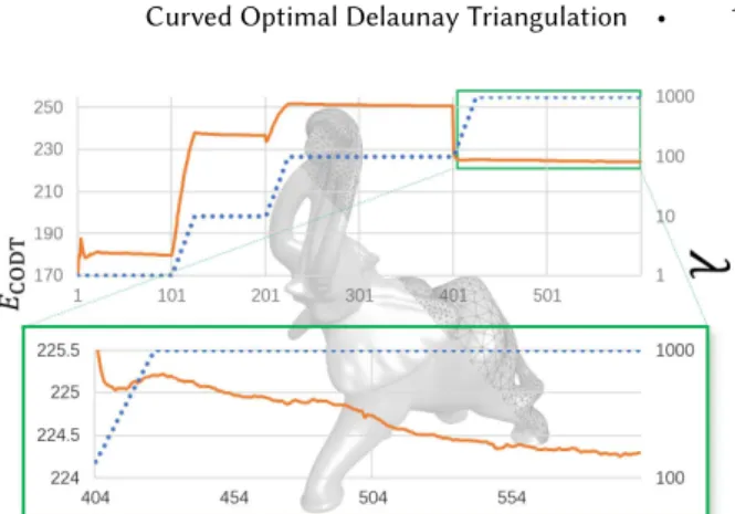
Fig. 14. Energy minimization. Energy plot (orange curve) and fi�ing strength scheduling (blue dots) during the meshing of the elephant model with 10K vertices, throughout the 600 rounds of optimization (horizontal axis). A closeup of the final stage is shown below. An energy drop is seen at the 401st round, where the mesh starts to curve.

energy increases; if stays constant for a while, then the energy decreases as the mesh deforms to improve the shape of its elements; �nally, increasing the order of the Bézier elements allows for a lowering of the energy as more DOFs become available. Fig. 14 shows the energy throughout the construction of the elephant mesh as increases. When we switch from PWL to quadratic elements (after 400 iterations), the energy drops precipitously.

Timings. We measured our timings on HP Z420 workstation, with a quadcore E5-1620-0 clocked at 3.6GHz and 16 GBytes of memory. We parallelized most steps of our CODT minimization using OpenMP in shared memory mode. Optionally, the compute-intensive evaluation of the energy and its gradient at internal and boundary cubature points are performed on GPU, bringing an ac-celeration of around a factor 5 on a NVIDIA GTX 1060. Compared to Optimal Delaunay (linear) Tetrahedralizations, curved meshing is more compute-intensive, even more so when the order of the elements increases. The complete process for meshing the skin sur-face shown in Fig. 1 with 200 vertices and order 3, takes nearly 50s. Each quasi-Newton iteration takes 0.03s in the linear stage, and 0.14s in the order-3 stage (we go directly from degree 1 to degree 3). Meshing the ManHead model with 1K vertices and order-3 takes less than 40 mins (but only 15 mins on GPU). Going up to 10K vertices increases the computational time to 6 hours (only 80 mins on GPU); each order-1 iteration then takes 0.41s (0.27s with GPU), while an order-3 iteration takes 5s (1s with GPU), and we observe a near-linear time complexity in the order to the Bézier simplices for each iteration. In our experiments the total number of rounds required for convergence depends heavily on the number of vertices, the domain complexity and the grading of the sizing �eld. Using a uniform sizing function is usually 20% faster or more, as the CODT energy and its derivatives are simpler to evaluate. In practice, we found that almost two thirds of the meshing time is used to reach convergence for n =1: once this stage is obtained, the rest (further degree elevations) goes relatively fast. Within each stage, most of the time is spent in computing cubatures and boundary �tting forces (hence the large time improvements when GPU acceleration is used). While we have not tried to fully optimize computational time, using