Selective Sweep at a QTL in a Randomly Fluctuating Environment

HAL Id: hal-02347347

https://hal.archives-ouvertes.fr/hal-02347347

HAL is a multi-disciplinary open access

archive for the deposit and dissemination of sci-entific research documents, whether they are pub-lished or not. The documents may come from teaching and research institutions in France or abroad, or from public or private research centers.

L’archive ouverte pluridisciplinaire HAL, est destinée au dépôt et à la diffusion de documents scientifiques de niveau recherche, publiés ou non, émanant des établissements d’enseignement et de recherche français ou étrangers, des laboratoires publics ou privés.

Selective Sweep at a QTL in a Randomly Fluctuating

Environment

Luis-Miguel Chevin

To cite this version:

Luis-Miguel Chevin. Selective Sweep at a QTL in a Randomly Fluctuating Environment. Genet-ics, Genetics Society of America, 2019, 213 (3), pp.987-1005. �10.1534/genetics.119.302680�. �hal-02347347�

1

Selective Sweep at a QTL in a Randomly Fluctuating Environment

Centre d’Ecologie Fonctionnelle et Evolutive (CEFE), CNRS, University of Montpellier, University of

6

Paul Valéry Montpellier 3, EPHE, IRD, Montpellier, France. 7

8 9

UMR 5175, 1919 Route de Mende, 34293 Montpellier Cedex 5, France. 10

E-mail: [email protected] 11

2

Abstract

12

Adaptation is mediated by phenotypic traits that are often near continuous, and undergo selective 13

pressures that may change with the environment. The dynamics of allelic frequencies at underlying 14

quantitative trait loci (QTL) depend on their own phenotypic effects, but also possibly on other 15

polymorphic loci affecting the same trait, and on environmental change driving phenotypic selection. 16

Most environments include a substantial component of random noise, characterized by both its 17

magnitude and its temporal autocorrelation, which sets the timescale of environmental predictability. I 18

investigate the dynamics of a mutation affecting a quantitative trait in an autocorrelated stochastic 19

environment that causes random fluctuations of an optimum phenotype. The trait under selection may 20

also exhibit background polygenic variance caused by many polymorphic loci of small effects 21

elsewhere in the genome. In addition, the mutation at the QTL may affect phenotypic plasticity, the 22

phenotypic response of given genotype to its environment of development or expression. Stochastic 23

environmental fluctuations increases the variance of the evolutionary process, with consequences for 24

the probability of a complete sweep at the QTL. Background polygenic variation critically alters this 25

process, by setting an upper limit to stochastic variance of population genetics at the QTL. For a 26

plasticity QTL, stochastic fluctuations also influences the expected selection coefficient, and alleles 27

with the same expected trajectory can have very different stochastic variances. Finally, a mutation may 28

be favored through its effect on plasticity despite causing a systematic mismatch with optimum, which 29

is compensated by evolution of the mean background phenotype. 30

31

Keywords: Fluctuating selection, stochastic environment, temporal autocorrelation, polygenic 32

adaptation, phenotypic plasticity. 33

3

Introduction

35

The advent of population genomics and next-generation sequencing has fostered the hope that the 36

search for molecular signatures of adaptation would reach a new era, wherein the recent evolutionary 37

history of a species would be inferred precisely and somewhat exhaustively, and fine details of the 38

genetics of adaptation would be revealed (Stapley et al. 2010). Despite undisputable successes, the 39

picture that has emerged in the last decade is more complex. First, the importance of polygenic 40

variation in adaptation has been re-evaluated based on theoretical and empirical arguments (Chevin 41

and Hospital 2008; Pavlidis et al. 2008; Pritchard et al. 2010; Rockman 2012; Jain and Stephan 2017; 42

Stetter et al. 2018; Höllinger et al. 2019), and methods have been designed to detect subtle frequency 43

changes at multiple loci that may jointly cause substantial phenotypic evolution (Turchin et al. 2012; 44

Berg and Coop 2014; Stephan 2016; Wellenreuther and Hansson 2016; Racimo et al. 2018; Josephs et 45

al. 2019). Consistent with (but not limited to) polygenic adaptation is the idea that mutations

46

contributing to adaptive evolution do not necessarily start sweeping when they arise in the population, 47

but may instead segregate for some time in the population and contribute to standing genetic variation, 48

before they become selected as the environment changes (Barrett and Schluter 2008; Kopp and 49

Hermisson 2009; Matuszewski et al. 2015; Jain and Stephan 2017). After the factors governing such 50

“soft sweeps” and their influence on neutral polymorphism have been characterized (Hermisson and 51

Pennings 2005; Przeworski et al. 2005), the debate has shifted to their putative prevalence in 52

molecular data, and perhaps more importantly to their contribution to adaptive evolution (Jensen 2014; 53

Garud et al. 2015; Hermisson and Pennings 2017). 54

Another line of complexity in the search for molecular footprints of adaptation comes from 55

temporal variation in selection. The classical hitchhiking model (Maynard-Smith and Haigh 1974; 56

Stephan et al. 1992) posits a constant selection coefficient without specifying its origin. Some models 57

have gone a step further by explicitly including a phenotype under selection, and have shown that even 58

in a constant environment, selection at a given locus may change over the course of a selective sweep, 59

as the mean phenotype in the background evolves through the effects of other polymorphic loci, in a 60

form of whole-genome epistasis mediated by the phenotype (Lande 1983; Chevin and Hospital 2008; 61

Matuszewski et al. 2015). In addition, selection is likely to vary in time because of a changing 62

environment. Most environments exhibit substantial fluctuations over time, beyond any trend or large 63

shifts (Stocker et al. 2013). These fluctuations are likely to affect natural selection, which emerges 64

from an interaction of the phenotype of an organism with its environment. Interestingly, one of the 65

first attempts to measure selection through time in the wild revealed substantial fluctuations in strength 66

and magnitude (Fisher and Ford 1947), spurring a heated debate about the relative importance of drift 67

versus selection in evolution, and setting the stage for the neutralist-selectionist debate (Wright 1948; 68

Kimura 1968; Yamazaki and Maruyama 1972; Gillespie 1977). Other iconic examples of adaptive 69

evolution also show clear evidence for fluctuating selection (Lynch 1987; Grant and Grant 2002; Bell 70

4 2010; Bergland et al. 2014; Nosil et al. 2018), suggesting that selection in natura is rarely purely 71

directional, but instead often includes some component of temporal fluctuations. Part of these 72

fluctuations involve deterministic, periodic cycles, such as seasonal genomic changes in fruit flies 73

(Bergland et al. 2014), but random environmental variation also certainly plays a substantial role. In 74

fact, virtually all natural environments exhibit some stochastic noise, characterized not only by its 75

magnitude but also by its temporal autocorrelation, which determines the average speed of fluctuations 76

and the time scale of environmental predictability (Halley 1996; Vasseur and Yodzis 2004). The 77

influence of such environmental noise on natural populations is attested notably by stochasticity in 78

population dynamics (Lande et al. 2003; Ovaskainen and Meerson 2010), and natural selection at the 79

phenotypic level has also been estimated as a stochastic process in a few case studies (Engen et al. 80

2012; Chevin et al. 2015; Gamelon et al. 2018). 81

Population genetics theory has a long history of investigating randomly fluctuating selection. In 82

particular, Wright (1948) used diffusion theory to derive the stationary distribution of allelic 83

frequencies in a stochastic environment, which was later extended to find the probability of quasi-84

fixation in an infinite population (Kimura 1954), and of fixation in a finite population (Ohta 1972). 85

This topic gained prominence during the neutralist-selection debate, where the relative influences of 86

genetic drift vs a fluctuating environment as alternative sources of stochasticity in population genetics 87

was strongly debated with respect to the maintenance of polymorphism and molecular heterozygosity 88

(Nei 1971; Gillespie 1973, 1977, 1979, 1991; Nei and Yokoyama 1976; Takahata and Kimura 1979), a 89

question that remains disputed in the genomics era (Mustonen and Lassig 2007, 2010; Miura et al. 90

2013). Another line of research has asked what is the expected relative fitness of a 91

genotype/phenotype in a fluctuating environment, and whether Wright’s (1937) adaptive landscape 92

could be extended to this context (Lande 2007; Lande et al. 2009). 93

However, this literature is mostly disconnected from the literature on adaptation of quantitative 94

traits to a randomly changing environment (Bull 1987; Lande and Shannon 1996; Chevin 2013; Tufto 95

2015). Even in work that investigates fluctuating selection both at a single locus and on a quantitative 96

trait (e.g. Lande 2007), the selection coefficient at the single locus is often postulated ad hoc, rather 97

than stemming from its effect on a trait under selection. Connallon and Clark (2015) recently 98

investigated the influence of a randomly fluctuating optimum phenotype on the distribution of fitness 99

effects of mutations affecting a trait, but they assumed non-autocorrelated fluctuations, and did not 100

derive the stochastic variance of the population genetic process, which is important driver of 101

probabilities of (quasi-)fixation (Kimura 1954; Ohta 1972). They also did not consider fitness epistasis 102

caused by evolution of the mean background phenotype. Lastly, this work has largely ignored possible 103

mutation effects on phenotypic plasticity, the phenotypic response of a given genotype to its 104

environment of development or expression (Schlichting and Pigliucci 1998; West-Eberhard 2003), 105

which is expected to evolve in environments that fluctuate with some predictability (Gavrilets and 106

Scheiner 1993a; Lande 2009; Tufto 2015). Instead, Connallon and Clark (2015) included a form of 107

5 environmental noise in phenotypic expression that is similar to bet hedging (Svardal et al. 2011; Tufto 108

2015). 109

I here extend a model that combines population and quantitative genetics (Lande 1983; Chevin and 110

Hospital 2008) to the context of an autocorrelated random environment causing movements of an 111

optimum phenotype, to ask: What is the distribution of allelic frequencies at a QTL in a stochastic 112

environment? How does it depend on whether a mutation is segregating alone, or instead affects a 113

quantitative trait with polygenic background variation? How does environmental stochasticity affect 114

the probability of a complete sweep at the QTL, and the resulting genetic architecture of the trait? And 115

how are these effects altered when the mutation affects phenotypic plasticity? 116

Model

Fluctuating selection

The core assumption of the model is that adaptation is mediated by a continuous, quantitative trait 119

undergoing stabilizing selection towards an optimum phenotype that moves in response to the 120

environment, as typical in models of adaptation to a changing environment (reviewed by Kopp and 121

Matuszewski 2014). More precisely, the expected number of offspring in the next generation 122

(assuming discrete non-overlapping generations) of individuals with phenotype is 123

(1)

where is the optimum phenotype at generation , and is the width of the fitness peak, which 124

determines the strength of stabilizing selection. The height of the fitness peak may affect

125

demography but not evolution, as it is independent of the phenotype. 126

In line with other models of adaptation to changing environments (Kopp and Matuszewski 2014), I 127

assume that the environment causes movement of the optimum phenotype, but does not affect the 128

width of the fitness function. The environment undergoes stationary random fluctuations, which may 129

be combined initially to a major, deterministic environmental shift of the mean environment. The 130

stochastic component of variation in the optimum is assumed to be autocorrelated, in the form of a 131

first-order autoregressive process (AR1) with stationary variance and autocorrelation over unit 132

time step (one generation). This is one of the simplest forms of autocorrelated continuous process: it is 133

Markovian (memory over one time step only), leading to an exponentially decaying autocorrelation 134

function with half-time generations. 135

Genetics

For simplicity, I base the argument on a haploid model, but much of the findings extend to diploids, 137

with a few additional complications such as over-dominance caused by selection towards an optimum 138

(Barton 2001; Sellis et al. 2011). I focus on a mutation at a locus affecting the quantitative trait – i.e., a 139

6 quantitative trait locus, or QTL -, with additive haploid effect on the trait. More precisely, I consider 140

a bi-allelic QTL, with mean phenotype m for the wild-type (ancestral) allele, in frequency , 141

and m + for the mutant (derived) allele, in frequency p. We are not interested here in the origin and 142

initial spread of the mutation from initially very low, drift-dominated frequencies. Investigating this 143

would require extending theory of fixation probabilities in changing environments (Uecker and 144

Hermisson 2011) to include environmental stochasticity, which is beyond the scope of this work. 145

Instead, the focus is here on adaptation from standing genetic variation, and the aim will be to track 146

the evolutionary trajectory of a focal mutation at a bi-allelic locus, starting from a low initial frequency 147

where most of frequency change can be attributed to selection. We will briefly address the 148

influence of drift at the end of the analysis. 149

Two types of genetic scenarios will be contrasted. In the “monomorphic background” scenario, no 150

other polymorphic locus affects the quantitative trait when the focal mutation is segregating at the 151

QTL. This corresponds to a form of strong selection weak mutation approximation (SSWM Gillespie 152

1983, 1991). This scenario requires no further assumption about the reproduction system (sexual or 153

asexual). In the opposite “polygenic background” scenario, variation in the trait is assumed to be 154

caused by a large number of weak-effect loci (or “minor genes”), in addition to the effect of the QTL 155

(or “major gene”). Sexual reproduction is assumed, with fertilization closely followed by meiosis over 156

a short diploid phase where selection can be neglected. I further assume that minor genes are at 157

linkage equilibrium among themselves and with the major gene, such that the genotypic background 158

has a similar distribution for all alleles at the major gene. Following standard quantitative genetics 159

(Falconer and MacKay 1996; Lynch and Walsh 1998), I assume that additive genetic values in the 160

background are normally distributed, with mean phenotype m and additive genetic variance G, and 161

that phenotypes also include a residual component of variation independent from genotype, with mean 162

0 and variance Ve. This model of major gene and polygenes, which takes its roots in Fisher’s (1918) 163

foundational paper for quantitative genetics, has been analyzed for evolutionary genetics by Lande 164

(1983), and later used to investigate selective sweeps at a QTL in constant environment or following 165

an abrupt environmental shift by Chevin and Hospital (2008). I here extend this work to a randomly 166

changing environment. 167

Phenotypic plasticity

I also investigate the case where both the mean background phenotype and the QTL effect may 169

respond to the environment, via phenotypic plasticity. Let be a normally distributed environmental 170

variable (e.g. temperature, humidity…) with mean and variance , which affects the development 171

or expression of the trait. Assuming a linear reaction norm for simplicity, the mean background 172

phenotype is 173

7 where is the slope of reaction norm, which quantifies phenotypic plasticity, and the intercept is 174

the trait value in a reference environment where by convention. I neglect evolution of plasticity 175

in the background for simplicity, and therefore assume that is a constant, while is a polygenic 176

trait with additive genetic variance G as before. The additive effect of the mutation at the QTL is also 177

phenotypically plastic, such that 178

(3)

with the additive increase in plasticity caused by the mutation at the QTL, and the additive 179

effect on the trait in the reference environment. 180

The environment of development partly predicts changes of the optimum phenotype for selection, 181

such that 182

(4)

where is normal deviate independent from , with mean 0 and variance , such that 183

the variance of optimum remains . Note that eq. (4) does not necessarily imply a causal relationship 184

between and , because selection occurs after development/expression of the plastic phenotype and 185

is thus likely to be influenced by a later environment (Gavrilets and Scheiner 1993a; Lande 2009). In 186

fact, the optimum may even respond to other environmental variables than , which jointly constitute 187

the cause of selection (Wade and Kalisz 1990; MacColl 2011), but can be partly predicted by upon 188

development. In this case is the product of the regression slope of the optimum on the causal 189

environment for selection, times the regression slope of this causal environment on the environment of 190

development (de Jong 1990; Gavrilets and Scheiner 1993a; Chevin and Lande 2015). When the same 191

environmental variable affects development and selection but at different times, then the latter 192

regression slope is simply the autocorrelation of the environment between development and selection 193

within a generation (Lande 2009; Michel et al. 2014). 194

Evolutionary dynamics

Lande (1983) has shown that the joint dynamics of a major gene and normally distributed polygenes in 196

response to selection are governed by a couple of equations that are remarkably identical to their 197

counterpart without polygenes and without a major gene, respectively. In other words, Wright’s (1937) 198

fitness landscape for genes and Lande’s (1976) fitness landscape for quantitative traits jointly apply in 199

the context of major gene combined with polygene. For a haploid sexual population, the recursions for 200

the allelic frequency p of the mutation at the major gene and for the mean phenotype m in the 201

polygenic background are then 202

(5)

8 where the partial derivatives are selection gradients on allelic frequency and mean phenotype, 203

respectively (Wright 1937; Lande 1976). 204

With selection towards an optimum as modeled in equation (1), and an overall phenotype 205

distribution that is a mixtures of two Gaussians with same variance and modes separated by the 206

effect of the major gene , the mean fitness in the population is 207

(7) where is the strength of stabilizing selection. Combining eqs (6) and (7), the selection 208

gradient on the mean background phenotype is 209

(8)

As in classical models of moving optimum for quantitative traits (Lande 1976; Kopp and Hermisson 210

2007), directional selection on the trait is proportional to the deviation of the mean phenotype from the 211

optimum, multiplied by the strength of stabilizing selection, which is larger when the fitness peak is 212

narrower. However here, the overall mean phenotype depends on , the frequency after selection of 213

the mutation at the QTL. This causes a coupling of dynamics in the background and at the QTL. 214

For the dynamics at the QTL it will be convenient to focus on the logit allelic frequency of the 215

mutation, . With a constant selection coefficient s as assumed in classical models of 216

selective sweeps, would increase linearly in time with slope s (Stephan et al. 1992), while 217

changes non linearly in time even in a constant environment if the mutation is dominant/recessive 218

(Teshima and Przeworski 2006), or if it affects a quantitative trait with polygenic background 219

variation as assumed here (Chevin and Hospital 2008). Combining eqs. (5) and (7), after some simple 220

algebra the recursion for over one generation of selection is 221

(9)

Note that is a measure of the selection coefficient s for this generation (Chevin 2011). In a constant 222

environment where for all t, the system admits two stable equilibria with fixation at the QTL, 223

, ,

(10)

and one unstable internal equilibrium 224

(11)

in line with previous analysis of the diploid version of this model (Lande 1983). Note that the mean 225

background phenotype evolves to compensate for the effect of the major gene, such that the overall 226

mean phenotype is at the optimum in all three equilibria, . 227

9

Approximation for weak fluctuating selection at QTL

228

The full model with coupled dynamics at the major gene and background polygenes can be used for 229

numerical recursions, but to make further analytical progress, I rely on an approximation of this model 230

that neglects the influence of the QTL on the background mean phenotype, as in previous analysis in 231

a constant environment (Chevin and Hospital 2008). In a randomly fluctuating environment, this 232

approximation consists of assuming that selection at the QTL is sufficiently weak that its contribution 233

to fluctuating selection on the mean background phenotype can be neglected, such that variance in the 234

directional selection gradient is proportional to 235

(12)

and similarly for its covariance across generations. 236

Simulations

The mathematical analysis of this model is complemented by population-based simulations under a 238

randomly fluctuating optimum. These simulations are based on recursions of equations (5-7), 239

assuming a constant additive genetic variance G in the background. In each simulation, the optimum is 240

initially drawn from an normal distribution with mean 0 and variance , and optima in subsequent 241

generations are drawn using , where is a standard normal deviate, such

242

that has stationary variance and autocorrelation as required. In simulations with phenotypic 243

plasticity, the environment of development is drawn retrospectively from the optimum, using 244

, where is drawn from a standard normal, such that has variance 245

and the regression slope of on is , as required (eq. 4). In simulations with background genetic 246

variance, the system is left to evolve for 500 generations, to allow the mean background phenotype to 247

reach a stationary distribution with respect to the fluctuating environment. The initial frequency at the 248

QTL is set then to , and the mean optimum is shift by relative to the expected background mean 249

phenotype, representing an abrupt environmental shift in the mean optimum at time 0. To simulate 250

random genetic drift, the allelic frequency at the QTL in the next generation is drawn randomly from a 251

binomial distribution with parameters (the effective population size) and (the expected 252

frequency after selection in the current generation), consistent with a haploid Wright-Fisher population 253

(Crow and Kimura 1970). Similarly for the mean background, genetic drift was simulated by drawing 254

the mean phenotype in the next generation from a normal distribution with mean the expected mean 255

background phenotype after selection, and variance (Lande 1976). 256

Data availability

A Mathematica notebook including code for simulations is available from a FigShare repository. 258

10

Results

259

We are interested in fluctuating selection at a gene affecting a quantitative trait (or QTL) exposed to a 260

randomly moving optimum phenotype. The stochastic population genetics at the QTL will be analyzed 261

on the logit scale for mathematical convenience (as in, e.g., Kimura 1954; Gillespie 262

1991), and also because this directly relates to empirical measurements (Chevin 2011; Gallet et al. 263

2012; see also Discussion). From equation (9), t generations after starting from an initial logit 264 frequency , we have 265 (13)

The first term in brackets increases linearly with time, and corresponds to a component of selection 266

that only depends on the phenotypic effect of the mutation and the strength of selection on the trait, 267

but not on the background phenotype or the environment. All the influence of the fluctuating 268

environment and background phenotype arises through the sum (second term in brackets), which 269

shows that the influences of all past maladaptations (deviations of the mean phenotype from the 270

optimum) weigh equally in their contribution to population genetics over time, over the range of allelic 271

frequencies for which drift can be neglected. In a stochastic environment, this means that a chance 272

event causing a large deviation from the optimum can have persistent effects on genetic change. This 273

occurs here because selection is assumed to be frequency independent; with frequency-dependent 274

selection, non-linear dynamics could instead rapidly erase memory of past environments and 275

maladaptation, as occurs for population dynamics with density dependence (Chevin et al. 2017). 276

The optimum phenotype is assumed to follow a Gaussian process. In most contexts we will 277

investigate, this causes the population genetics at the QTL to also follow a Gaussian process on the 278

logit scale, such that has a Gaussian distribution at any time. A Gaussian distribution of logit allelic 279

frequency was also found in phenomenological models without an explicit phenotype, where selection 280

coefficients were assumed to undergo a Gaussian process (Kimura 1954; Gillespie 1991, p.149). The 281

reason for this correspondence is that is linear in phenotypic mismatches with optimum in eq. (13), 282

and these mismatches themselves follow a Gaussian process (i) in the absence of background 283

polygenic variation; and (ii) with background polygenic variation, as long as evolution of the mean 284

background is little affected by the QTL, such that . When these assumptions 285

hold, the distribution of allelic frequencies in a stochastic environment can be summarized by their 286

mean and variance on the logit scale, and . A simple transformation can then be used to retrieve 287

the distribution of allelic frequencies, following Gillespie (1991, p.149), 288

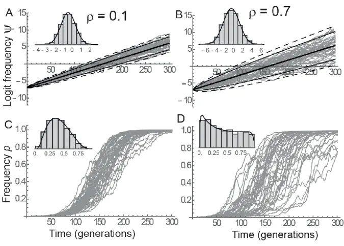
(14) where is the density of a normal distribution with mean E and variance V evaluated at x. This

289

transformation is illustrated in Figure 1. 290

11

Non-plastic QTL

291

We first focus on the situation where the phenotypic effect of the mutation at the QTL does not 292

change in response to the environment. The environment is assumed to undergo a sudden shift at time 293

0 in addition to the stochastic fluctuations, such that the expected mean background phenotype 294

initially deviates from the expected optimum by , and that a mutation approaching 295

the mean phenotype from the average optimum is expected to be favored. 296

Monomorphic background: It is informative to first investigate the simplest case where the trait

297

does not have background polygenic variation. The focal mutation at the QTL then segregates in a 298

population that is otherwise monomorphic with respect to adaptation to the fluctuating environment. 299

This context belongs to the weak-mutation limit often assumed in molecular evolution, for instance in 300

Gillespie’s (1983, 1991) SSWM regime, and establishes the most direct connection with results from 301

earlier models of fluctuating selection that do not include an explicit phenotype under selection 302

(Wright 1948; Kimura 1954; Nei 1971; Ohta 1972; Gillespie 1973, 1979, 1991; Nei and Yokoyama 303

1976; Takahata and Kimura 1979). With monomorphic background, from eq. (13) the expected logit 304

allelic frequency at time t starting from a known frequency is 305

In this context, the expected logit allelic frequency thus increases linearly in time, with a slope given 306

by the expected selection coefficient . This selection coefficient is not 307

affected by random fluctuations in the optimum, and instead only depends on the constant mismatch 308

between the background mean phenotype and the expected optimum . The mutation at the 309

QTL is expected to spread in the population only if it allows approaching the optimum, that is, if 310

. 311

Even though fluctuations in the optimum do not affect the expected trajectory, they do increase the 312

variance of the stochastic population genetic process. The variance of logit allelic frequency at time t, 313

starting from a known frequency

,

When the optimum undergoes a stationary AR1 process as assumed here, the variance of the 315

population genetic process at the QTL becomes 316 (17)

where is the stationary variance of random fluctuations in the optimum, and is their 317

autocorrelation over one generation. Note that in this scenario, is also the per-generation 318

12 autocorrelation of selection coefficients , while the variance of selection coefficients is 319

. For large times , eq. (17) further simplifies as 320

(18)

which shows that the variance in logit allelic frequency eventually increases near to linearly with time 321

(Figure 3A), and converges more rapidly to this linear change under smaller autocorrelation in the 322

optimum. Stochastic variance in the optimum increases faster under larger autocorrelation in the 323

optimum. Figure 1 shows that the distribution of is well predicted by a Gaussian with mean and 324

variance given by eqs. (15) and (17). Increasing environmental autocorrelation does not change the 325

expected evolutionary trajectory on the logit scale, but increases its variance (Figure 1A-B). When 326

transforming to the scale of allelic frequencies, increased environmental autocorrelation causes a 327

broadening of the time span over which selective sweeps occur in the population (Figure 1C-D). 328

Polygenic background: With polygenic variation in the background, the mean background

329

phenotype is no longer constant, but instead evolves in response to deterministic and stochastic 330

components of environmental change. Away from the unstable equilibrium in eq. (11), the expected 331

evolutionary trajectory at the QTL is similar to that investigated without fluctuating selection (Lande 332

1983; Chevin and Hospital 2008). In particular, when the influence of the QTL on evolution of the 333

background trait can be neglected, then combining eqs. (6) and (8) the expected mean background 334

phenotype approaches the expected optimum geometrically, (Lande 335

1976; Gomulkiewicz and Holt 1995). Combining with eq. (13), the expected logit allelic frequency is 336

. (19)

This shows that even when a mutation at the QTL is initially beneficial because it points towards the 337

optimum, its dynamics slows down in time as the mean background approaches the optimum (Lande 338

1983; Chevin and Hospital 2008). Equation (19) even predicts that an initially beneficial mutation 339

eventually becomes deleterious, and starts declining in frequency when the mean background is 340

sufficiently close to the optimum that the QTL causes an overshoot of the latter (Lande 1983; Chevin 341

and Hospital 2008). This can be seen by noting that in the long run, the term in parenthesis in eq. (19) 342

tends towards and eventually becomes dominated by , leading to an expected 343

dynamics that declines linearly with slope . An initially beneficial mutation starts declining 344

when its selection coefficient crosses 0. Applying the weak-effect approximation for evolution of the 345

mean background (above eq. 19) to eq. (9), this occurs when , that is, at time 346

.

(20)

At this point, the expected logit allelic frequency of the mutation at the QTL reaches its maximum, 347

which is (combining eqs. 20 and 19) 348

13 . (21)

However, this scenario may actually be avoided if the focal mutation reaches ( ) before 349

, such that the system gets beyond the unstable equilibrium in eq. (11). The mutation at the QTL

350

then sweeps to fixation, and the mean background evolves away from the optimum to compensate for 351

the QTL effect (Lande 1983; Chevin and Hospital 2008). We will investigate this scenario in more 352

detail below, but let us first turn to the variance of the stochastic process. 353

For the variance of the process, we rely on the weak-effect approximation in eq. (12), whereby 354

fluctuating selection on the mean background phenotype is little affected by dynamics at the QTL. 355

More broadly speaking, we assume the system is away from the unstable equilibrium in eq. (11). 356

When this holds, we can build upon previous evolutionary quantitative genetics results for the 357

dynamics of the mean background phenotype in a fluctuating environment, to derive the dynamics at 358

the QTL. For an AR1 process as modeled here, the stationary variance of mismatch of the mean 359

background phenotype with the optimum is (Charlesworth 1993) 360

(22)

and its temporal autocorrelation function over  generations is 361

(23)

where (Cotto and Chevin 2019; see also continuous-time approximation in Chevin and 362

Haller 2014). Combining with eq. (16) leads, after some algebra, to the stochastic variance of logit 363 allelic frequency, 364 (24)

Quite strikingly, contrary to the case of a monomorphic genetic background, does not increase 365

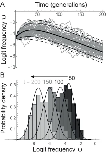
indefinitely with polygenic background; instead, its dynamics slows down towards an asymptotic 366 maximum, 367 (25) In other words, with a polygenic background, the distribution of logit allelic frequency at the QTL 368

tends to a traveling wave, i.e. a Gaussian with moving mean but constant variance, as shown in Figure 369

2. This property holds as long as the population is not near the unstable equilibrium in eq. (11), and

370

frequencies at the QTL are sufficiently intermediate that drift is not the main source of stochasticity 371

(below). 372

Inspection of eq. (24) indicates that the rate of approach to the asymptotic variance is determined 373

by the smallest of and . In realistic parameter ranges, the rate of response to selection in the 374

background is small, while may be well below 1, so the time scale of approach to equilibrium for 375

14 should scale in . This is confirmed by the simulations, which show that converges 376

faster to its asymptote under larger background genetic variance, while the rate of convergence is little 377

affected by (Figure 3). The asymptotic variance may be well below that in the absence of polygenic 378

background variation (compare panel A to B-C in Figure 3). As predicted by eq. (25), the asymptotic 379

variance decreases with increasing genetic variance in the background, and increases with 380

increasing environmental autocorrelation (Figure 3). The influence of autocorrelation is highly non-381

linear: in our example is approximately doubled from to , but multiplied by 4-5 382

from to (Figure 3 B-C). As expected, eq. (24) converges to its equivalent with no 383

background polygenic variation (eq. 17) in the limit of small genetic variance ( ), as illustrated 384

in Figure 3D. 385

The variance of the stochastic population genetic process has consequences for the bistability of 386

genetic architecture, and the likelihood of a complete sweep. In particular, when the expected 387

trajectory in eq. (19) reaches the vicinity of the unstable equilibrium in eq. (11), the process variance 388

may cause paths to split on each side of this equilibrium and reach alternative fixed equilibria, with 389

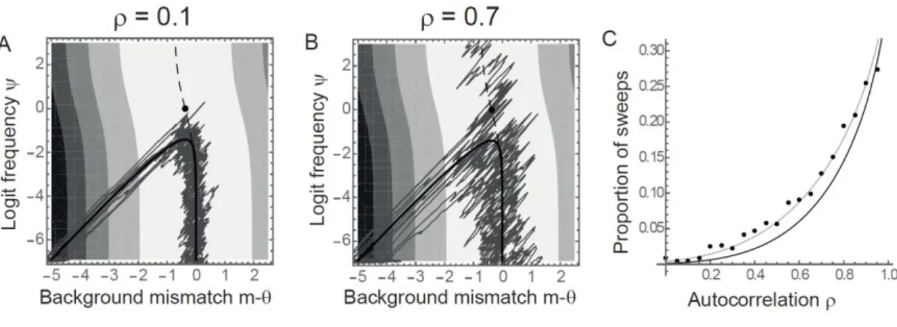
either complete sweep or loss of the mutation at the QTL (eq. 10). This is illustrated in Figure 4. In 390

this example, the expected trajectory involves a loss of the mutation at the QTL, which occurs for all 391

sample paths shown in Figure 4A. However, increasing environmental autocorrelation causes some 392

trajectories to sweep to high frequency (Figure 4B). This occurs because environmental 393

autocorrelation increases the stochastic variance of the population genetic process (eqs. 24, 25), and 394

thereby the probability that some trajectories cross the unstable equilibrium, reaching the basin of 395

attraction of the high-frequency equilibrium. Based on this rationale, the proportion of trajectories that 396

reach each alternative stable equilibrium (fixation or loss) may be approximated from the expected 397

proportion of trajectories that are above and below the unstable equilibrium, based on the predicted 398

Gaussian distribution of at time , when the expected frequency is predicted to be highest based 399

on the simplified model where the QTL does not affect evolution of the mean background (eq. 20). 400

Figure 4C shows that this approach correctly predicts how the proportion of sweeps changes with

401

environmental autocorrelation . Importantly, since the expected trajectory does not depend on 402

stochastic environmental fluctuations (neither nor appear in eq. 19), all effects of environmental 403

autocorrelation (or variance) on the probability of a sweep are mediated by the stochastic variance of 404

the process. 405

QTL for phenotypic plasticity

Let us now turn to the case where the QTL influences not only the phenotype, but also how this 407

phenotype responds to the environment. Phenotypic plasticity, the phenotypic response of a given 408

genotype to its environment of development or expression, is a ubiquitous feature across the tree of 409

life (Schlichting and Pigliucci 1998; West-Eberhard 2003). There is also massive evidence for genetic 410

15 variance in plasticity in the form of genotype-by-environment interactions, one of the oldest and most 411

widespread observations in genetic studies (Falconer 1952; Via and Lande 1985; Scheiner 1993; 412

Gerke et al. 2010; Des Marais et al. 2013), with molecular mechanisms that are increasingly 413

understood (Angers et al. 2010; Beldade et al. 2011; Ghalambor et al. 2015; Gibert et al. 2016). For 414

simplicity I here assume linear reaction norms, where the slope quantifies plasticity. Although this is 415

necessarily a simplification of reality, it is generally a good description over relevant environmental 416

ranges for phenological traits, a major class of phenotypic responses to climate change (e.g., 417

Charmantier et al. 2008). This also allows comparing our results to the large body of theoretical 418

literature also based on the assumption of linear reaction norms (Gavrilets and Scheiner 1993b; 419

Scheiner 1998; Lande 2009; Chevin and Lande 2015; Tufto 2015). Such models likely capture the 420

broad evolutionary effects of plasticity for monotonic reaction norms. More complex monotonic 421

reaction norm shapes can be modeled to focus on more specific scenarios such as threshold traits with 422

a bounded range of expression (Chevin and Lande 2013), while non-monotonic reaction norms with 423

an optimum are more appropriate for fitness or performance traits (Lynch and Gabriel 1987; Huey and 424

Kingsolver 1989), which are not the focus here. I also assume for simplicity that the background has 425

constant plasticity, such that all genetic variance in plasticity comes from the major gene. A final 426

assumption in this section will be to focus on stationary environmental fluctuations with no major shift 427

( ). Such purely stationary fluctuations are expected to counter-select any mutation at the major 428

gene in the absence of plasticity (eqs. 15 and 19), so it is a good benchmark on which to assess 429

selection on a plasticity QTL. 430

Monomorphic background: In the low mutation limit where the background mean phenotype does

431

not evolve while the mutation is segregating at the QTL, but has still evolved on a longer time scale to 432

match the expected optimum at the onset of selection at the QTL, the expected logit allelic frequency 433

increases linearly in time as in eq. (15), with expected selection coefficient (Appendix) 434

(26)

The first term in curly brackets is a component of selection that does not depend on the pattern of 435

environmental fluctuations, and is similar to the expected selection coefficient without plasticity (15) 436

and without a major environmental shift. This component reduces the expected selection coefficient, 437

as it increases the mismatch with the expected optimum phenotype. The second term is a component 438

of selection caused by the effect of the QTL on phenotypic plasticity. This term shows that the plastic 439

effect of the mutation at the QTL is favored by selection if it allows approaching the optimal 440

response to the environment of development , that is if . The expected 441

selection coefficient is maximum for , regardless of . Importantly, whereas the 442

expected selection coefficient on a non-plastic mutation does not depend on the variance of 443

fluctuations (eq. 15), the component of the expected selection coefficient caused by plasticity is 444

16 stronger under larger variance of the environment of development, and thus depends on 445

fluctuations in the optimum (from eq. 4). This reflects the fact that, in a stationary environment, 446

selection on phenotypic plasticity stems from its effect on the variance of phenotypic mismatch with 447

the optimum, rather than on the average mismatch (Lande 2009; Ashander et al. 2016). As the 448

variance of the environment of development increases, a mutation with a given beneficial effect on 449

phenotypic plasticity becomes increasingly likely to spread even if it causes a systematic mismatch 450

with the optimum in the mean environment, with a deleterious side-effect . In the absence of 451

background genetic variation, the expected selection at the plasticity QTL does not depend directly on 452

autocorrelation in the environment, but only on the dependence of the optimum on the environment of 453

development, through the parameter . Note however that if phenotypic development/expression and 454

movements of the optimum respond to the same environmental variable (e.g. temperature), but at 455

different times in a generation, then is directly related to the autocorrelation of the optimum 456

(Lande 2009; Michel et al. 2014). 457

The variance of selection coefficients with plasticity but no background genetic variation is 458

.

(27)

Equation (27) implies that mutations that have the same expected selection coefficient, because they 459

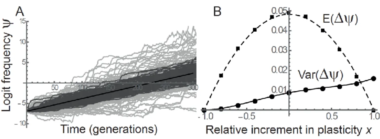
cause the same deviation from the optimal plasticity , can have different variances in allelic 460

frequency change. This is illustrated in Figure 5, which shows that a mutation that leads to hyper-461

optimal plasticity has more stochastic variance than a mutation that cause equally sub-optimal 462

plasticity, because the former causes overshoots of the optimum while the latter causes undershoots. 463

This difference in stochastic variance between mutations with the same expected selection coefficient, 464

which should impact their relative probabilities of quasi-fixation (Kimura 1954), is stronger for larger 465

deviation from the optimal plasticity (Figure 5B). 466

Polygenic background: When the mean background phenotype also evolves via polygenic variation,

467

the expected dynamics at the QTL are modified in two main ways. First, background genetic variance 468

contributes to adaptive tracking of the mean phenotype via genetic evolution, thus reducing the benefit 469

of phenotypic plasticity, as in pure quantitative genetic models (Tufto 2015). The level of plasticity 470

that maximizes the expected selection coefficient then becomes (Appendix) 471

(28)

where the last term is the regression slope of the background mean reaction norm intercept on the 472

environment of development, caused by evolution of the mean background in response to the 473

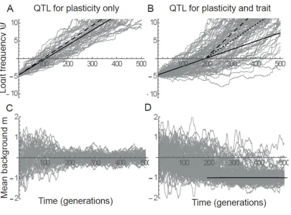
fluctuating environment. Figure 6A illustrates how selection via the QTL effect on plasticity is 474

reduced by adaptive tracking of the optimum by evolution of the mean background. 475

17 Second, when the benefit of plasticity allows the mutation at the QTL to spread despite a 476

pleiotropic effect on the intercept of the reaction norm, the expected mean background phenotype 477

can evolve away from the optimum in the average environment to compensate for the associated cost, 478

that is, it evolves to (Figure 6D). Intriguingly, after this has occurred the mutation at the 479

QTL becomes more strongly selected than if it did not have a pleiotropic effect on the reaction norm 480

intercept (Figure 6B). This occurs because the QTL effect on reaction norm intercept now allows 481

compensating for maladaptation in the background, which adds a positive component to the 482

benefit via the QTL effect on phenotypic plasticity. In other words, what initially caused a 483

displacement from the mean optimum allows approaching the mean optimum after the mean 484

background has been displaced. Furthermore, the spread of the mutation at the plasticity QTL reduces 485

the effective magnitude of fluctuating selection on background mean reaction norm intercept, resulting 486

in smaller evolutionary fluctuations in the background (Figure 6C, D). 487

Drift versus fluctuating selection

All the analytical results above neglect the influence of random genetic drift, and simulations were run 489

under large to single out the influence of fluctuating selection as a source of stochasticity. 490

However, it is useful to delineate more precisely the conditions under which drift can be neglected 491

relative to environmental stochasticity. The overall variance in allelic frequency change, accounting 492

for both fluctuating selection and random genetic drift in a Wright-Fisher population, can be obtained 493

from the law of total variance, and was previously shown (Ohta 1972) to be 494

(29)

where is the variance of selection coefficients caused by fluctuating selection. From this 495

it entails that fluctuation selection dominates drift as a source of stochasticity when , that is 496 for 497 (30)

This can be translated into a condition for the logit allelic frequency , 498 (31)

Very similar results are obtained (not shown) if the criterion is based on the stochastic variance of , 499

for which the fluctuating selection component is independent of (as derived in the main text), but 500

the drift component is not. Equation (31) shows that an absolute condition for fluctuating selection to 501

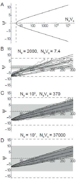
be the dominant source of stochasticity is When this holds, fluctuating selection dominates 502

18 over a range of intermediate allelic frequencies, while drift dominates at extreme frequencies outside 503

of this range. The bounds of this range are entirely determined by the compound parameter , as 504

shown by eqs. (30-31) and Figure 7A. Figure 7 further illustrates that for small , small initial 505

frequencies and/or large final frequencies result in inflated variance relative to the expectation under 506

pure fluctuating selection (panels B-C), as well as fixation events by drift (panel B). As increases 507

from panel B to D, the predictions under pure fluctuating selection become increasingly accurate, all 508

the more so as the initial allelic frequency is within the range defined by eq. (31). 509

Discussion

Analysis of a simple model combining population and quantitative genetics has revealed a number of 511

interesting properties about fluctuating selection at a gene affecting a quantitative trait (or QTL), when 512

this trait undergoes randomly fluctuating selection caused by a moving optimum phenotype. The first 513

important observation is that, when assessed on the logit scale - a natural scale for allelic frequencies 514

(Kimura 1954; Gillespie 1991; Chevin 2011; Gallet et al. 2012) -, the dynamics at the QTL has a 515

simple connection to movements of the optimum, since the selection coefficient depends linearly on 516

the mismatch between the mean background phenotype and the optimum (eq. 9; see also Martin and 517

Lenormand 2006). For a QTL that has the same phenotypic effect in all environments (no phenotypic 518

plasticity), the expected trajectory only depends on the expected phenotypic mismatch with the 519

optimum, not on the pattern of fluctuations in this optimum. However the variance of trajectories, an 520

important determinant of probabilities of quasi-fixation (Kimura 1954), is strongly affected not only 521

by the magnitude of fluctuations in the optimum, but also by their autocorrelation (eq. 17, Figure 1). 522

When the focal QTL is the only polymorphic gene undergoing fluctuating selection, this stochastic 523

variance increases linearly over time (Figure 3A), at a rate that is faster under larger positive 524

autocorrelation in the optimum. In contrast, when polygenic variation elsewhere in the genome allows 525

for evolution of the mean background phenotype, stochastic variance at the QTL is bounded by a 526

maximum asymptotic value, which is lower under higher genetic variance in the background (eqs. 24-527

25 and Figure 3 B-C). This stochastic variance caused by fluctuating selection interacts with the 528

inherent bi-stability of genetic architecture in this system (Lande 1983; Chevin and Hospital 2008), 529

and may increase the probability that the mutation at the QTL reaches fixation at the expense of the 530

background mean phenotype (as illustrated in Figure 4), or the reverse. 531

When the mutation at the QTL also affects phenotypic plasticity via the slope of a linear reaction 532

norm, then even its expected trajectory depends on the pattern of fluctuations, with stronger selection 533

under large fluctuations (eq. 26), contrary to the case of a non-plastic QTL. Interestingly, mutations 534

with the same expected selection coefficient - because they cause the same deviation from the optimal 535

plasticity – may have very different variances in allelic trajectories, depending on whether they tend to 536

cause overshoots or undershoots of the fluctuating optimum (Figure 5). Finally, a mutation that is 537

19 sufficiently strongly selected via its effect on phenotypic plasticity can spread despite causing a 538

systematic mismatch with the optimum in the average environment. When the mean background 539

phenotype can evolve by polygenic variation, it can compensate for this pleiotropic effect on reaction 540

norm intercept. Quite strikingly, this increases selection at the plasticity QTL, causing the mutation to 541

spread faster than if it only affected plasticity (Figure 6B). 542

Consistent with previous uses of this model with a major gene and polygenes (Lande 1983; 543

Agrawal et al. 2001; Chevin and Hospital 2008; Gomulkiewicz et al. 2010), I did not model explicitly 544

the maintenance of genetic variance in the background, instead assuming that it had reached an 545

equilibrium between mutation and stabilizing/fluctuating selection. This has provided simple and 546

robust analytical insights about the interplay of selection at a major gene with background polygenic 547

variation. Although environmental fluctuations should affect the expected additive genetic variance G 548

to some extent (Burger and Gimelfarb 2004; Svardal et al. 2011), this does not necessarily affect our 549

results because they are conditioned on G, rather than on mutational variance for instance, which is 550

less directly amenable to empirical measurement. More critical is the fact that the background additive 551

genetic variance should itself fluctuate in time as alleles in the background change in frequency, 552

especially in a finite population (Bürger and Lande 1994; Höllinger et al. 2019). This should increase 553

temporal variation in the evolutionary process, so that results about stochastic variance here may be 554

considered as lower bounds, if the long-term mean G is used in formula. Modeling explicitly the 555

dynamics of background quantitative genetic variance in a random environment would require using 556

individual-based simulations, as done for instance by Bürger and Gimelfarb (2002). Previous work 557

based on a similar environmental context as modeled here proved that most results are little affected in 558

regimes where substantial genetic variation can be maintained for a quantitative trait (Chevin and 559

Haller 2014; Chevin et al. 2017), as assumed here. 560

Although the simulations included random genetic drift, all the analytical results were derived by 561

neglecting the influence of drift. These analytical results are therefore valid over a range of allelic 562

frequencies that is entirely determined by the product of the effective size by the variance of selection 563

coefficients, as shown in eqs. (30-31) and Figure 7. In most simulations, I have assumed that the 564

mutation at the QTL is initially at low frequency, but still common enough to be within the range 565

defined by eqs. (30-31), where frequency change is entirely driven by selection. It would be 566

worthwhile investigating in future work the probability of establishment of a mutation that starts in 567

one copy and affects a trait exposed to randomly fluctuating selection, but this requires developments 568

that are beyond the scope of the present study. For our purpose, we can consider that the initial 569

frequency p0 stems either from the trajectory of a newly arisen mutation conditional on non-extinction,

570

which is expected to rapidly rise away from 0 (Barton 1998; Martin and Lambert 2015), or from a 571

distribution at mutation-selection drift equilibrium (Wright 1937; Barton 1989; Höllinger et al. 2019). 572

Our analytical results about the distribution of logit allelic frequency lend themselves well to 573

comparisons with empirical measurements. Indeed the logit of allelic frequencies is readily obtained 574

20 from number of copies of each type, since , where and are the 575

copy numbers of the mutant (derived) and wild-type (ancestral) allele, respectively. In fact, when 576

frequencies are estimated on a subsample from the population, the strength of selection on genotypes 577

is generally estimated using logistic regression (Gallet et al. 2012), a generalized linear (mixed) model 578

that uses the logit as link function. Our theoretical predictions therefore apply directly to the linear 579

predictor of such a GLMM, without requiring any transformation. For instance if we consider an 580

experiment where multiple lines undergo independent times series of a stochastic environment (i.e., 581

different paths of the same process), the stochastic variance among replicates can be estimated as a 582

random effect in a logistic GLMM. If multiple loci are available, this random effect should strongly 583

covary among loci within an environmental time series, because they share the same history of 584

environments, in contrast to frequency changes caused by drift, which should only be similar between 585

tightly linked loci. 586

The results here are based on a model of fluctuating optimum for a quantitative trait, similar to 587

previous theory by Connallon and Clark (2015), but extend this theory by allowing for environmental 588

autocorrelation, and by deriving the stochastic variance of the population genetic process. Importantly, 589

most of the present results should also be relevant to cases where an explicit phenotype under selection 590

is not identified or measured, but the relationship between fitness and the environment has the form of 591

a function with an optimum, which can be approximated as Gaussian (Lynch and Gabriel 1987; 592

Gabriel and Lynch 1992; Gilchrist 1995). For many organisms, especially microbes, measuring 593

individual phenotypes can be challenging, and it may prove difficult to identify most traits involved in 594

adaptation to a particular type of environmental change (ie temperature, salinity…). A common 595

solution is to directly measure fitness or its life-history components (survival, fecundity) across 596

environments, to produce an environmental tolerance curve (Deutsch et al. 2008; Thomas et al. 2012; 597

Foray et al. 2014). An influence of the history of previous environments on these tolerance curves can 598

also be included, via plasticity-mediated acclimation effects (Calosi et al. 2008; Gunderson and 599

Stillman 2015; Nougué et al. 2016). It has been highlighted previously that tolerance curves can be 600

thought of as emerging from a moving optimum phenotype on unmeasured, possibly plastic, 601

underlying traits (Chevin et al. 2010; Lande 2014), so that a simple re-parameterization can translate 602

all the results above in terms of evolution of tolerance breadth and environmental optimum. Such a 603

connection has recently been invoked to analyze population dynamics in a stochastic environment 604

(Chevin et al. 2017; Rescan et al. 2019), suggesting that results from the current study are not 605

restricted to cases where relevant quantitative traits under fluctuating selection can be measured, but 606

may instead apply to a broad range of organisms exposed to randomly changing environments. 607

21

Acknowledgements

608

This work was supported by the European Reseach Council (Grant 678140-FluctEvol). I thank J. 609

Hermisson and three anonymous reviewers for useful criticisms and suggestions. 610

Literature cited

Agrawal A. F., E. D. Brodie, and L. H. Rieseberg, 2001 Possible consequences of genes of major 612

effect: transient changes in the G-matrix. Genetica 112: 33–43. 613

Angers B., E. Castonguay, and R. Massicotte, 2010 Environmentally induced phenotypes and DNA 614

methylation: How to deal with unpredictable conditions until the next generation and after. Mol. 615

Ecol. 616

Ashander J., L.-M. Chevin, and M. L. Baskett, 2016 Predicting evolutionary rescue via evolving 617

plasticity in stochastic environments. Proc. R. Soc. B Biol. Sci. 283. 618

Barrett R. D. H., and D. Schluter, 2008 Adaptation from standing genetic variation. Trends Ecol. Evol. 619

Barton N., 1989 The Divergence of a Polygenic System Subject to Stabilizing Selection, Mutation and 620

Drift. Genet. Res. 54: 59–77. 621

Barton N. H., 1998 The effect of hitch-hiking on neutral genealogies. Genet. Res. Cambridge 72: 123– 622

33. 623

Barton N. H., 2001 The role of hybridization in evolution. Mol. Ecol. 10: 551–568. 624

Beldade P., A. R. Mateus, and R. A. Keller, 2011 Evolution and molecular mechanisms of adaptive 625

developmental plasticity. Mol Ecol 20: 1347–1363. 626

Bell G., 2010 Fluctuating selection: the perpetual renewal of adaptation in variable environments. 627

Philos. Trans. R. Soc. B-Biological Sci. 365: 87–97. 628

Berg J. J., and G. Coop, 2014 A Population Genetic Signal of Polygenic Adaptation. PLoS Genet. 629

Bergland A. O., E. L. Behrman, K. R. O’Brien, P. S. Schmidt, and D. A. Petrov, 2014 Genomic 630

Evidence of Rapid and Stable Adaptive Oscillations over Seasonal Time Scales in Drosophila. 631

PLoS Genet. 632

Bull J. J., 1987 Evolution of Phenotypic Variance. Evolution (N. Y). 41: 303–315. 633

Burger R., and A. Gimelfarb, 2004 The effects of intraspecific competition and stabilizing selection on 634

a polygenic trait. Genetics 167: 1425–1443. 635

Bürger R., and R. Lande, 1994 On the Distribution of the Mean and Variance of a Quantitative Trait 636

under Mutation-Selection-Drift Balance. Genetics 138: 901–912. 637

Bürger R., and A. Gimelfarb, 2002 Fluctuating environments and the role of mutation in maintaining 638

quantitative genetic variation. Genet. Res. 80: 31–46. 639

Calosi P., D. T. Bilton, and J. I. Spicer, 2008 Thermal tolerance, acclimatory capacity and 640

vulnerability to global climate change. Biol Lett 4: 99–102. 641

Charlesworth B., 1993 Directional selection and the evolution of sex and recombination. Genet. Res. 642

22 61: 205–224.

643

Charmantier A., R. H. McCleery, L. R. Cole, C. Perrins, L. E. Kruuk, et al., 2008 Adaptive phenotypic 644

plasticity in response to climate change in a wild bird population. Science (80-. ). 320: 800–803. 645

Chevin L.-M., and F. Hospital, 2008 Selective sweep at a quantitative trait locus in the presence of 646

background genetic variation. Genetics 180: 1645–60. 647

Chevin L.-M., R. Lande, and G. M. Mace, 2010 Adaptation, plasticity, and extinction in a changing 648

environment: Towards a predictive theory. PLoS Biol. 8. 649

Chevin L.-M., 2011 On measuring selection in experimental evolution. Biol. Lett. 7: 210–213. 650

Chevin L.-M., 2013 Genetic constraints on adaptation to a changing environment. Evolution (N. Y). 651

67. 652

Chevin L.-M., and R. Lande, 2013 Evolution of discrete phenotypes from continuous norms of 653

reaction. Am. Nat. 182. 654

Chevin L.-M., and B. C. Haller, 2014 The temporal distribution of directional gradients under 655

selection for an optimum. Evolution (N. Y). 68. 656

Chevin L.-M., and R. Lande, 2015 Evolution of environmental cues for phenotypic plasticity. 657

Evolution (N. Y). 69. 658

Chevin L.-M., M. E. Visser, and J. Tufto, 2015 Estimating the variation, autocorrelation, and 659

environmental sensitivity of phenotypic selection. Evolution (N. Y). 69: 2319–2332. 660

Chevin L.-M., O. Cotto, and J. Ashander, 2017 Stochastic Evolutionary Demography under a 661

Fluctuating Optimum Phenotype. Am. Nat. 190: 786–802. 662

Connallon T., and A. G. Clark, 2015 The distribution of fitness effects in an uncertain world. 663

Evolution (N. Y). 69: 1610–1618. 664

Cotto O., and L.-M. Chevin, 2019 FLUCTUATIONS IN LIFETIME SELECTION IN AN 665

AUTOCORRELATED ENVIRONMENT. J. Evol. Biol. submitted. 666

Crow J. F., and M. Kimura, 1970 An Introduction to Population Genetics Theory. Harper and Row, 667

New York. 668

Deutsch C. A., J. J. Tewksbury, R. B. Huey, K. S. Sheldon, C. K. Ghalambor, et al., 2008 Impacts of 669

climate warming on terrestrial ectotherms across latitude. Proc Natl Acad Sci U S A 105: 6668– 670

6672. 671

Engen S., B. E. Saether, T. Kvalnes, and H. Jensen, 2012 Estimating fluctuating selection in age-672

structured populations. J. Evol. Biol. 25: 1487–1499. 673

Falconer D. S., 1952 The problem of environment and selection. Am. Nat. 293–298. 674

Falconer D. S., and T. F. MacKay, 1996 Introduction to quantitative genetics. Longman Group, 675

Harlow, UK. 676

Fisher R. A., 1918 The correlation between relatives on the supposition of Mendelian inheritance. 677

Trans. R. Soc. Edinburgh 52: 35–42. 678

Fisher R. A., and E. B. Ford, 1947 The spread of a gene in natural conditions in a colony of the moth 679