• Aucun résultat trouvé

Tropical extra-tropical thermocline water mass exchanges in the Community Climate Model v.3 Part I: the Atlantic Ocean

N/A
N/A
Protected

Academic year: 2021

Partager "Tropical extra-tropical thermocline water mass exchanges in the Community Climate Model v.3 Part I: the Atlantic Ocean"

Copied!
11
0
0

Texte intégral

(1)

HAL Id: hal-00331140

https://hal.archives-ouvertes.fr/hal-00331140

Submitted on 10 Oct 2006

HAL is a multi-disciplinary open access

archive for the deposit and dissemination of

sci-entific research documents, whether they are

pub-lished or not. The documents may come from

teaching and research institutions in France or

abroad, or from public or private research centers.

L’archive ouverte pluridisciplinaire HAL, est

destinée au dépôt et à la diffusion de documents

scientifiques de niveau recherche, publiés ou non,

émanant des établissements d’enseignement et de

recherche français ou étrangers, des laboratoires

publics ou privés.

exchanges in the Community Climate Model v.3 Part I:

the Atlantic Ocean

Ilana Wainer, Alban Lazar, Amy Solomon

To cite this version:

Ilana Wainer, Alban Lazar, Amy Solomon. Tropical extra-tropical thermocline water mass exchanges

in the Community Climate Model v.3 Part I: the Atlantic Ocean. Ocean Science, European Geosciences

Union, 2006, 2 (2), pp.137-146. �10.5194/os-2-137-2006�. �hal-00331140�

(2)

Ocean Sci., 2, 137–146, 2006 www.ocean-sci.net/2/137/2006/

© Author(s) 2006. This work is licensed under a Creative Commons License.

Ocean Science

Tropical extra-tropical thermocline water mass exchanges in the

Community Climate Model v.3 Part I: the Atlantic Ocean

I. Wainer1, A. Lazar2, and A. Solomon3

1Department of Physical Oceanography, University of S˜ao Paulo, S˜ao Paulo, Brazil 2Laboratoire d’Oc´eanographie Dynamique et de Climatologie (LODYC), Paris, France

3National Oceanic Atmospheric Administration-Cooperative Institute Research Environmental Sciences (NOAA-CIRES)

Climate Diagnostics Center, USA

Received: 12 December 2005 – Published in Ocean Sci. Discuss.: 10 May 2006 Revised: 8 August 2006 – Accepted: 20 September 2006 – Published: 10 October 2006

Abstract. The climatological annual mean

tropical-extra-tropical pathways of thermocline waters in the Atlantic Ocean are investigated with the NCAR CCSM numerical coupled model. Results from three numerical experiments are analyzed: Two are fully coupled runs with different spa-tial resolution (T42 and T85) for the atmospheric component. The third numerical experiment is an ocean-only run forced by NCEP winds and fluxes. Results show that the different atmospheric resolutions have a significant impact on the sub-duction pathways in the Atlantic because of how the wind field is represented. These simulation results also show that the water subducted at the subtropics reaching the EUC is entirely from the South Atlantic. The coupled model ability to simulate the STCs is discussed.

1 Introduction

Perhaps one of the most interesting characteristics of the tropical-extra-tropical circulation in the Tropical Atlantic Ocean is the fact that most of the water reaching the equa-tor has Southern Hemisphere origin, in particular within the Equatorial Undercurrent (EUC) i.e. Zhang et al. (2003); Molinari et al. (2003). This is accomplished due to the equa-torward flow at the depth of the thermocline by the Subtrop-ical Cells (STC). This shallow overturning cell (confined to the upper 500 m, according to Schott et al., 1998; Snowden and Molinari, 2003; Zhang et al., 2003) is characterized by poleward Ekman flow at the surface, associated upwelling and a return flow which is associated with the subduction processes that transfer interior ocean water into the thermo-cline. In other words, Ekman pumping injects surface water into intermediate depths along isopycnal surfaces in the sub-tropics that ventilate the sub-tropics.

Correspondence to: I. Wainer

(wainer@usp.br)

Zhang et al. (2003), using geostrophic velocities derived from hydrographical data, describe the mean pathways in the interior and surface ocean for tropical-extra-tropical water exchange. They show that in the North Atlantic, water path-ways go around the potential vorticity ridge located under the Intertropical Convergence Zone converging on the western boundary. In the Southern Hemisphere the ventilation path-ways are spread throughout the interior and include a west-ern boundary route. Their observational analysis will serve as comparison basis for the model simulations analyzed in this work. Their work is described in Snowden and Molinari (2003) who provide a comprehensive review of the Atlantic STC. They point out that in general there is still much to be learned about its variability and structure mostly because of the uneven data distribution and lack of quantitative errors surrounding them. Grodsky and Carton (2002), attempt to look at the near-surface pathways of the Atlantic STC using drifter data. They discuss that the small number of drifters along with their inhomogeneous spatial and temporal distri-bution, are not enough to quantify the relative importance of the four major pathways they identified. In their study the water exiting the cold tongue region does not lead directly back to the subduction regions.

The modeling studies that have been carried out; i.e. Lazar et al. (2002); Malanotte-Rizzoli et al. (2000); Blanke et al. (1999), are ocean only numerical experiments that provide a global description of the pathways associated with the STC circulation. Lazar et al. (2002), and Malanotte-Rizzoli et al. (2000) based their study on the evaluation of the Bernoulli function on isopycnal surfaces, showing that for the South Atlantic STC, nearly all the thermocline flow from the sub-tropics into the equator passes through the western boundary. In a high resolution modeling study, Harper (2002) using par-ticle trajectories, shows that the subducted water reaching the EUC is entirely from Southern Hemisphere origin. Results of these numerical simulations show considerable differences in the mean pathways within the STCs. These differences can

(3)

be attributed to differences in model configurations, differ-ences in the simulated MOC (because the STC can be super-imposed on its return northward branch and hard to distin-guish one from the other) and the wind forcing chosen (see for example, Inui et al., 2002).

In this qualitative study, the annual subduction rate, up-welling and Lagrangian (subsurface) trajectories at different isopycnals are examined in order to quantify the STC path-ways similar to Lazar et al. (2002)

2 The numerical model

Coupled models used in climate change studies have under-gone a rapid development in recent years and have in sev-eral respects obtained a considerable degree of realism. The CCSM3 (Community Climate System Model) is a numeri-cal coupled model, composed of 4 components: atmosphere, ocean, land surface and sea-ice. The on-line description can be found at: http://www.ccsm.ucar.edu/models/ccsm3.0. The CCSM3 system includes new versions of all the compo-nent models. The atmosphere is CAM version 3.0 (Collins et al., 2006), the land surface is CLM version 3.0 (Oleson et al., 2004; Dickinson et al., 2005), the sea ice is CSIM version 5.0 (Briegleb et al., 2004), and the ocean is based upon POP version 1.4.3 (Smith and Gent, 2002). New features in each of these components are described in Collins et al. (2006). Each component is designed to conserve energy, mass, total water, and fresh water in concert with the other components. The dynamical atmosphere model is the Community At-mosphere Model (CAM3, Collins et al., 2005), a global atmospheric general circulation model developed from the NCAR CCM3. In this work, two horizontal resolutions are used both have 26 vertical levels. One has triangular trunca-tion at 42 wave numbers (T42) and the other 85 (T85) which roughly corresponds to a horizontal resolution of 3.75◦ and 1.4◦, respectively. The hybrid vertical coordinate merges a terrain-following sigma coordinate at the bottom surface with a pressure-level coordinate at the top of the model.

The ocean component solves the primitive equations in general orthogonal coordinates in the horizontal with the hydrostatic and Boussinesq approximations. The grid uses spherical coordinates in the southern hemisphere, but in the northern hemisphere the pole is displaced into Greenland at 80◦N, 40◦W. The horizontal grid has 320 (zonal) × 384 (meridional) grid points, and the resolution is uniform in the zonal, but not in the meridional, direction. In the southern hemisphere, the meridional resolution is 0.27◦ at the

equa-tor, gradually increasing to 0.54◦at 33◦S, and is constant at higher latitudes. There are 40 levels in the vertical, whose thickness monotonically increases from 10 m near the sur-face to 250 m in the deep ocean. The minimum depth is 30 m, and the maximum depth is 5.5 km. The surface fresh water flux is converted into an implied salt flux using a con-stant reference salinity. Therefore, although the sea surface

height varies locally, the ocean volume remains fixed. The domain is global, which includes Hudson Bay, the Mediter-ranean Sea, and the Persian Gulf. The time step used is one hour, which is small enough that no Fourier filtering is re-quired around the displaced Greenland pole.

The horizontal viscosity is a Laplacian operator that is anisotropic following the formulation of Smith and McWilliams (2003), and uses different coefficients in the east-west and north-south directions. Both coefficients are spatially and temporally variable, depending on the local rates of shear and strain, and the minimum background hori-zontal viscosity is 1000 m2s−1. The vertical mixing scheme is the KPP scheme of Large et al. (1994). In the ocean in-terior, the background diffusivity varies in the vertical from 0.1×10⁻⁴m2 s−1 near the surface to 1.0×10⁻⁴m2 s−1 in the deep ocean. The background viscosity has the same ver-tical profile, but is a factor of ten larger. The parameteriza-tion of the effects of mesoscale eddies is that of Gent and McWilliams (1990), with a constant coefficient of 600 m2 s−1. Further details on the ocean component of the CCSM3 can be found in Smith and Gent (2002).

The Community Land Model, CLM (Dickinson et al., 2005), is the result of a collaborative project between sci-entists in the Terrestrial Sciences Section of the Climate and Global Dynamics Division (CGD) at NCAR and the CCSM Land Model Working Group. Other principal working groups that also contribute to the CLM are Bio-geochemistry, Paleoclimate, and Climate Change and Assessment. The land model grid is identical to the atmosphere model grid.

The sea-ice component of CCSM is the Community Sea-Ice Model (CSIM, Briegleb et al., 2004). The sea-ice com-ponent includes the elastic-viscous-plastic (EVP) dynam-ics scheme, an ice thickness distribution, energy-conserving thermodynamics, a slab ocean mixed layer model, and the ability to run using prescribed ice concentrations. It is sup-ported on high- and low-resolution Greenland Pole grids, identical to those used by the POP ocean model.

The coupled model data analyzed consists of annual av-erages of temperature, salinity and current velocity from 50 years of two 400 year runs of the NCAR CCSM where the atmosphere has different spatial resolution (T42, T85). The ocean only (POP3) data analyzed is the annual mean av-erage of a 43 year run forced by NCEP/NCAR winds and fluxes. The South Atlantic is defined by the region between the Equator and 55◦S and between 65◦W and 20◦E.

The uncoupled NCAR CCSM Ocean Model (POP3) is forced in a similar manner as when it is coupled to an atmo-spheric model. The open-ocean surface boundary conditions are fluxes of momentum, heat, and freshwater. The open-ocean turbulent heat fluxes are computed from a prescribed atmospheric state using traditional, bulk formulas. The re-quired surface winds, air temperature, and air humidity are obtained from the National Centers for Environmental Pre-diction (NCEP) global reanalysis data set; see Kalnay et al. (1996).

(4)

I. Wainer et al.: Tropical extra-tropical interaction in the CCSM 139 The numerical results are compared to the Levitus (Levitus

et al., 2000) climatology. Although this is the standard clima-tology for ocean model versus data inter-comparison, caution should be exercised in the equatorial region (where merid-ional gradients are large) considering the broad smoothing used.

Large and Danabasoglu (2006) discuss to great extent the biases in the coupled model associated with SST and sea surface salinity (SSS), their seasonal cycles and impact of the wind-driven circulation together with problems with the width, separation, and location of the western boundary cur-rents. This work goes a little further in an attempt to under-stand the biases in the model associated with the extratropical pathways of the thermocline waters in the Atlantic Ocean.

3 Results

3.1 The tropical annual mean circulation

An important feature of the tropical-extra-tropical dynamics is the Tropical Cell (TC) which is even shallower than the STC and confined to the tropics. As described in Molinari et al. (2003) they are associated with down-welling driven by the decrease of the poleward Ekman transport just a few degrees off the equator. STCs interact with the TCs. Figure 1 shows at 30◦W the mean meridional versus vertical velocity circulation vectors superimposed on the zonal velocity field (shading) characterizing the TC for the three numerical ex-periments. Selected isopycnals at 5 kg m−3intervals, repre-sented by white contours are also superimposed on Fig. 1. The common feature is the surface Ekman divergence and associated equatorial upwelling through the upper 50 m. The compensating geostrophic subsurface convergence is not so clear in the coupled runs (hereafter referred to as T42 and T85, respectively): there is a clear reversal of the surface poleward flow south of the equator below 100 m which is not observed north of the equator. There, the flow is significantly reduced, but not convergent. As a matter of fact, there is a maximum in the northward flow for these runs, at 80 m depth, centered exactly at the equator. The forced ocean result (hereafter referred to as POP3) shows the expected conver-gence associated with the TC at approximately 100 m. The Ekman-driven, divergent flow, at the equator, forces equato-rial upwelling and poleward surface flow to form a closed shallow subtropical cell.

Around 8◦S there is unrealistic upwelling in the coupled

models which can be related to an unrealistic wind field. In-deed, examination of the mean wind stress field in Fig. 4 shows that there is a sign reversal in the wind stress curl at 8◦S (positive in POP3 – Fig. 4c – and negative for the cou-pled model runs – Fig. 4a, b). The weak aonal winds in the coupled model results also account for the absence of a better defined northern SEC and the surfacing of the EUC.

Fig. 1. Mean meridional versus vertical velocity (x1e3) circulation vectors superimposed on the zonal velocity field (contour interval is 5 cm/s for T85 and T42 – upper panels – and 10 cm/s for POP3 – bottom panel). Thick white horizontal curves are selected isopyc-nals at 5 kg m−3contour intervals. Note that for each run a different isopycnal surface crosses the core of the EUC. Thick black line is the zero contour for zonal velocity (in color shading).

The mean zonal velocity at 30◦W (color shading) , with

the main isopycnals superimposed in Fig. 1 shows the east-ward flowing Equatorial Undercurrent (EUC) characterized by a strong velocity core around 100 m depth. Note that the core of the EUC lies in the density range between the 24.5 kg m−3<σθ<26.5 kg m−3isopycnal surfaces consistent

with Schott et al. (2004) and Molinari et al. (2003). However, for each simulation the core is located on a different isopy-cnal surface (24.3 kg m−3for T42, Fig. 1 left panel; 24.5 kg m−3for T85, Fig. 1 right panel and 25.0 kg m−3for POP3, bottom panel). Even though the 26.5 kg m−3 isopycnal is not explicitly plotted, only waters less or near it reaches the equator. Denser water do not seem t reach the EUC.

The velocity at the EUC core for the coupled numerical experiments has a maximum of approximately 40 cm/s. For the forced case the maximum velocity value of the EUC is at 112 m and approximately 10 cm/s stronger. It should be noted that the core is displaced slightly southward (and up-ward, at 83 m depth) in the coupled runs corresponding to an upper limit of the eastward flow at σθ=23.0 kg m−3 for the

T85 and 22.5 kg m−3for the T42 run which reaches the sur-face. This upper limit of 22.5 kg m−3is inferred based on the

interval spacing of the isopycnals in Fig. 1. The maximum EUC velocity for T42 and T85 occurs further west, at 34◦W,

reaching approximately 45 cm/s at 83 m depth. The depth of the EUC core coincides with the depth of the thermocline of the tropical Atlantic. The mean climatological temperature structure is shown in Fig. 2 for all three runs (b–d), together with the Levitus et al. (2000) climatological field (Fig. 2a) and their differences (Fig. 2e–h) at 30◦W. Equatorial cross-sections can be seen in Fig. 2i–k. A significant difference

(5)

Fig. 2. Climatological mean temperature (◦C) at 30◦W down to 300 m between 30◦S–30◦N for the (a) Levitus et al. (2000) Cli-matology, (b) POP3, (c) T42 (d) T85; their differences (e) POP3 – Levitus et al. (2000) Climatology, (f) POP3 – T42, (g) POP3 – T85 and (h) T85 – T42; and the equatorial sections for (i) POP3, (j) T42

(k) T85 (l) Levitus et al. (2000) Climatology.

between the forced numerical experiment (POP3) and the Levitus et al. (2000) climatology seen in Fig. 2e is right at the equator at the EUC core level (around 100 m depth) show-ing a 5◦C difference. A difference of 4◦C at 80 m depth, at the latitude where the eastward flowing North Equatorial Counter Current (NECC) encounters the westward flowing North Equatorial Current (NEC) is also noted. Differences between POP3 and the two coupled runs (Figs. 2f, g) show a model bias in the thermocline in the tropics descending to 300 m in the subtropics. Differences in both cases are significantly larger for the Northern Hemisphere subtropics with maximum values close to 8◦C at approximately 18◦N (within the region of the NEC). Small differences (compared to POP3) in the temperature profiles between the coupled runs show that T85 is warmer than T42 in the southern sub-tropics, the thermocline and the region poleward of 22◦N.

The core of the EUC has temperatures around 20◦C,

which is about 4–5◦C cooler than the surface waters in the

equatorial region. From the equatorial temperature sections (Fig. 2i–l) it is evident that the thermocline shoals eastward only in the POP3 run. It is actually almost flat for the coupled runs where there is a reverse east-west temperature gradient with warmer waters in the east. POP3 temperature distribu-tion is closer to the Levitus et al. (2000) Climatology albeit warmer in the surface. In the west (Fig. 2i–l) the thermocline is more diffuse and the 26◦C isotherm is very flat with re-spect to the observations. In Levitus et al. (2000) (Fig. 2l), this isotherm surfaces between 20◦W and 0◦W and is con-fined more to the west. At some points (e.g., 25◦W) it is locally steeper. The warm bias in the coupled model could also be a result of the too-weak equatorial upwelling.

With respect to the salinity structure, along the EUC pole-ward boundaries, relatively fresher waters are found (not shown), which can indicate that lower salinity waters may also feed the EUC and recirculate within the South Equato-rial Current (SEC). High South Atlantic Water (SAW) salin-ity values (greater than 36.6 psu) present within the POP3 EUC core agree with the discussion of (Bonhoure et al., 2003) about the direct SAW supply to the tropics through the North Brazil Current (NBC) retroflection.

The annual mean surface horizontal temperature distribu-tion for the three runs (contour interval is 2◦C) with the sur-face current velocity field superimposed can be seen in Fig. 3. The most realistic temperature field is that of POP3 (upper right panel) very similar to Levitus et al. (2000) (Fig. 3, up-per left panel), except for the absence of the eastern Atlantic upwelling off Africa, which is an already known bias. The marine stratus regions off the western coasts of North and South America and off Africa are too warm by 2–3 K, re-sulting from a bias in cloud simulation. According to Nor-ris and Weaver (2001) the atmospheric component of the CCSM overestimates shortwave and long wave cloud radia-tive forcing when vertical motion is upward (negaradia-tive omega) and underestimates shortwave and long wave cloud radia-tive forcing compared to observations when vertical motion

(6)

I. Wainer et al.: Tropical extra-tropical interaction in the CCSM 141

Fig. 3. Climatological mean Levitus et al. (2000), model sur-face temperature (contour interval is 2◦C) and current field vectors (cm/s).

is downward. The coupled model present a reverse gradi-ent in the equatorial region (noted by Davey et al., 2002, in an inter-comparison study of 23 different coupled models). Warmer temperatures are found in the eastern equatorial At-lantic rather than in the west as in observations.

The annual mean horizontal current velocity field for all three runs has overall similarities where one can delineate the two tropical gyres and major equatorial (North and South Equatorial Currents, Guyana Current) and western boundary currents (i.e. the North and South Brazil currents are very similar in magnitude for the three runs). The flow is less re-alistic in the coupled runs. In T42 (left bottom panel) the zonal current is predominantly westward south of the equa-tor but reverses right at the equaequa-tor extending for the whole width of the Atlantic. This can be interpreted as a southward displacement of the NECC that does not appear in the forced case (Fig. 3, lower panel). In T85 the flow at the equator is also eastward but weaker. In both cases this is due to the sur-facing of the EUC. At this latitude the largest zonal current velocity difference between POP3 and the coupled runs oc-curs at approximately 10◦–12◦W and is about −45 cm/s for POP3 minus T42 and −30 cm/s for POP3 minus T85. An-other difference in the annual mean velocity field between the coupled runs and the forced case is off Southern Africa in the eastern basin where there seems to be a spurious southward flowing current from approximately 5◦S to 25S in the

cou-pled runs that merges with the southern branch of the South Equatorial current whereas in POP3 this does not occur.

In order to appreciate some of the differences described, it is important to turn to the forcing. Since STCs are largely influenced by the winds, they are compared, together with the curl, between the three runs and shown in Fig. 4.

Fig. 4. Climatological mean wind stress (vectors) and curl (shaded

contours with interval of 0.5*0.1 N/m2) for the coupled runs T85 and T42 (a) and (b), respectively, and (c) POP3-NCEP, which is the forcing for the ocean component. Differences are shown in the right hand side panels: (d) shows the difference between the two coupled runs (T85–T42); (e) shows the difference between POP3 (NCEP wind stress) and T42 and (f) is the difference between POP3 and T85. Pink shading denotes negative wind stress curl.

The zonal winds are too weak at the equator which ac-counts for the weak upwelling in the coupled model noted earlier. Weaker winds are also responsible for the absence of a better defined Northern SEC and the surfacing of the EUC. Furthermore, the equatorial winds (off South Africa) are also too weak which accounts for the lack of coastal upwelling and the ill direction of the ocean currents there (i.e. Fig. 3).

It can be seen that the broad-scale spatial characteristics are very similar between the coupled (Figs. 4a, b) and forced run (POP3 – Fig. 4c) which is actually the NCEP wind stress. However, more detailed examination reveals that the largest differences are between POP3 and T42 (Fig. 4e). Overall, the curl (and consequently the associated Ekman-pumping velocity field) is significantly stronger in POP3 than in the coupled runs. However, the curl in T42 is stronger com-pared to POP3 north of the equator with the maximum dif-ference off the African coast of about 1.5 N/m2 off Mau-ritania (Fig. 4e). The same difference between POP3 and T85 is 1.0 N/m2(Fig. 4f). The other region with big differ-ences is also off the African coast but further south, between 15◦–25◦S. Differences between POP3 and T42 are also the largest reaching 1.5 N/m2off the coast of Namibia (Fig. 4e). It is interesting to note that in this region, the difference be-tween POP3 and T85 is significantly less (Fig. 4f, bebe-tween 0.5–1 N/m2). Comparison of the climatological mean wind

(7)

Fig. 5. Climatological mean absolute potential vorticity contours

(c.i.=10−10m−1 s−1) and Salinity in grams/kilogram projected onto the isopycnal surface that crosses EUC core as a function of longitude and latitude for (a) POP3 at σθ=25.3 (b) T85 at σθ =

24.0 kg/m3and (c) T42 at σθ=24.3 kg/m3. Also plotted for

refer-ence is (d) potential vorticity contours and salinity distribution from Levitus et al. (2000) at σθ=25.3. Salinity interval is 0.25.

stress curl between the coupled runs indeed shows that they differ largely in the south-eastern part of the domain. In T85 (Fig. 4d) the negative wind stress curl is stronger but confined to a narrow region hugging the coast of Namibia and Angola (much like the NCEP winds in POP3, Fig. 4c) whereas in T42 the same region is broader and extends further north-west. Note also that the zero line is displaced a few degrees west in T42 as compared to POP3 and T85. The importance of these differences becomes evident once the pathways of tropical extra-tropical exchange of thermocline waters, that are highly dependent on the wind distribution (e.g. Liu and Philander, 1995; Inui et al., 2002) are examined.

3.2 The subtropical cells

The STC can be viewed as an extension of the venti-lated thermocline theory (i.e. Snowden and Molinari, 2003; Malanotte-Rizzoli et al., 2000; Hazeleger et al., 2003; Luyten et al., 1983, etc.) where subtropical thermocline waters that are subducted along specified isopycnals conserve potential vorticity (PV) and are transported to the Equator. At the equator the wind forced upwelling and associated poleward flow are also part of the STC. The equatorward path of the STC is still subject of investigation and is complicated in the South Atlantic due to, among other factors, the superposition

of the northward flowing branch of the basin-wide merid-ional overturning circulation (MOC) that underlies the STC return flow at the western boundary.

One way to look at the characteristics of tropical-extra-tropical exchanges in the CCSM3 and to understand the pathways by which the STC feeds the EUC, is to ex-amine the planetary potential vorticity distribution (PV). Since water that upwells at the equator will originate from 24.5<σθ<26.8 kg/m3 and in order to compare with Zhang

et al. (2003), PV contours are plotted on the σθ=25.3 surface

and can be seen in Fig. 5 overlaying the salinity distribution on the same surface. PV and salinity for the coupled runs are also displayed in Fig. 5 but at σθ=24.3 kg/m3 for T42

and σθ=24.0 kg/m3for T85. The reason for using different

isopycnal surfaces is the fact that the core of the EUC is at a different depth for each run. The isopycnals chosen are ex-actly the ones that cross the EUC core at 30◦W, as seen in

Fig. 1.

The PV calculations follows the formulation of Cushman-Roisin (1987) as in Lazar et al. (2002) where PV can be ap-proximated by:

P V = f ρ0

∂ρ

∂z (1)

where f = Coriolis parameter and ρ = density.

The flow streamlines for each run, calculated at the isopy-cnal surfaces representing the depth of the EUC core (σθ=25,

24.5, 24.3 for POP3, T85 and T42, respectively) and shown in Fig. 6. The streamlines, show a distinct asymmetry be-tween hemispheres. For POP3 (lower panel), the interior pathways are observed only in the South Atlantic together with the western boundary route. There is a closed stream-line region northeast of the equator (between approximately 10◦N and 20◦N induced by the positive Ekman pumping (e.g. Fig. 4) which is a result of the PV ridge seen in Fig. 5. This implies that the subducted waters cannot cross the re-gion towards the equator in order to conserve PV. Instead they are advected westward. Depth of the σθ=25.3 surface

in-creases toward the western side of the basin (not shown) con-sistent between all three runs and in agreement with Lazar et al. (2002).

The southern hemisphere outcrop-line in the coupled runs is displaced poleward with respect to POP3. In the eastern Atlantic, there is a closed circulation which in part is as-sociated with the Angola Gyre, which is formed by one of the branches of the South Equatorial Current in the west, the South Equatorial Counter Current (SECC)and the Benguela Undercurrent (BUC). It can be noted that the Angola Gyre in the coupled runs is further South, off the coast of Namibia. There, within the model’s Angola Gyre, lies a region of en-hanced negative Ekman pumping (i.e. Fig. 4) and an associ-ated PV trough (Fig. 5). This scenario favors the equatorward flow of subtropical waters directed predominantly towards the western boundary. The circulation shown for POP3 re-sembles closely the results of Lazar et al. (2002) and Zhang

(8)

I. Wainer et al.: Tropical extra-tropical interaction in the CCSM 143 et al. (2002) which includes more uniform interior pathways

in the southern hemisphere. In the northern hemisphere the interior flow makes several turns before moving towards the equator going around the PV barrier (under the ITCZ). In other words, the PV field (Fig. 5) is characterized by the Ekman-pumping induced ridge, associated with the positive curl (Fig. 4) that forces the flow to go around it in a con-voluted way limiting the possibility of the existence of inte-rior water pathways in the northern hemisphere thermocline. Flow from the southern hemisphere in all numerical experi-ments reaches the northern hemisphere tropics through east-ward detours in the EUC, NEUC and NECC which is consis-tent with the review presented by Schott et al. (2004). Due to a limitation in the horizontal resolution it is not possible to observe any contribution due to ring shedding from the NBC retroflection. The North Equatorial Current (NEC), North Equatorial Counter Current (NECC), and Equatorial Under-current (NEUC) North Brazil Current (NBC) are dominant features of the STC circulation.

The pathways discussed above are also evident from the salinity distribution on the same isopycnal surfaces (Fig. 5, shading). The differences between the forced and coupled models become clear showing that less dense waters of the South Atlantic make their way into the tropical thermo-cline in the coupled model runs. Of the model runs, POP3 (Fig. 5a), shows both that the outcrop line is significantly equatorward (which means denser waters of the SAW makes its way into the thermocline) and contribution from both the north and south Atlantic to the equatorial circulation, al-though the contribution from the southern hemisphere is sig-nificantly larger. The salinity distribution and PV contours for Levitus et al. (2000) can be seen in Fig. 5d for reference. It is clear that the salinity distribution in POP3 (Fig. 5a) most resembles observations in Levitus et al. (2000). The salin-ity field is characterized by regions of high salinsalin-ity (salinsalin-ity maximum waters) in the North and South subtropical At-lantic ocean. In between these two regions of maximum salinity lies tropical low salinity waters. The coupled runs (Figs. 5b, c) exhibit a significantly different structure. The northern hemisphere salinity maximum region, for exam-ple, is displaced poleward and is confined to the west of 40◦W with a maximum value of approximately 37.5 psu. The equivalent high salinity waters of the southern hemi-sphere in the coupled runs is considerably less dense than in POP3 (approximately 1 psu difference). It is spatially con-fined to the western boundary, hugging the southeast coast of Brazil with its maximum value of approximately 36 psu centered around 22–23◦S. In POP3 the region of maximum

salinity in the southern hemisphere has a maximum of ap-proximately 37 psu that extends zonally across the whole basin centered around 10◦S. Basically this spatial distribu-tion translates into a salinity front in the northwest corner of the basin along the trajectory of the coupled model’s NBC (i.e. Fig. 3) while the equivalent for the forced model seems to follow the NEC (as in Zhang et al., 2002).

Fig. 6. Streamlines at the depth of the EUC core for each of the runs

at σθ=24.3 kg m−3and 24.5 kg m−3isopycnal surface for the T42

and T85 coupled runs (top panels, respectively) and at σθ=25.0 kg

m−3for POP3 (lower panel).

In summary, from the salinity distribution in Fig. 5 it can be clearly seen for POP3 that the high salinity subtropical waters does reach the EUC from both northern and south-ern Atlantic resulting in a high salinity tongue that extends eastward along the equator. For the coupled runs the equa-tor is not marked by the high salinity subtropical waters and contribution from the northern hemisphere subtropics is not evident.

3.3 Annual subduction

Next, the annual subduction is calculated as in Cushman-Roisin (1987), following Lazar et al. (2002), given by:

Sann= −(VH.∇H + wH), (2)

where VH and wH are the climatological annual mean

hor-izontal and vertical velocity at the depth H . H is the max-imum climatological mean mixed layer depth. Sann for the

three runs can be seen in Fig. 7. Warm color (reds) shading represents positive contours associated with downwelling. Negative values (blues) indicate entrainment into the mixed layer. The overall general structure is similar between the runs, however there are some distinct differences, particu-larly between the coupled runs (T42 and T85) and the forced case (POP3). The common feature between T42 and T85, and to some extent POP3 is the broad entrainment region (negative contours) particularly in the high positive PV re-gion in the east, in the Northern Hemisphere. In the west, between 5◦N–10◦N, at the NECC retroflection region, there is a strong region of positive values that are confined to the west of 30◦W in the T42 run (Fig. 7, upper left panel) and spreads towards the east in T85 (Fig. 7, upper right panel) and POP3 (Fig. 7, lower panel). Similar to the the numeri-cal study of Lazar et al. (2002), which would compare with

(9)

Fig. 7. Annual subduction rate Sannfor the three runs. Region with warm colors (reds, orange and yellow) correspond to positive values (subduction). Contour interval is m/year. Top panels: T42 (left) and T85 (right). Bottom panel: POP3.

POP3 in this study, the Southern Hemisphere shows a more regular distribution with respect to the northern hemisphere. Compared to POP3, the equatorial upwelling signature in T42 is weak and confined to the west. At T85 a more basin-wide signal is observed. These characteristics are best ob-served in the vertical velocity field at the climatological mean maximum mixed layer depth shown in Fig. 8. Regional dif-ferences of upwelling/downwelling can be observed which imply that the atmospheric model resolution seems to affect the strength and spatial features of the STC/TC system. Con-sidering that the annual subduction rate is largely affected by the strength and distribution of the wind fields (e.g. Inui et al., 2002; Lazar et al., 2002; Liu and Philander, 1995) the response is expected to be different. Using the forced case as a realistic base for comparison, i.e. the POP3 results are in good agreement with the observation analysis of Zhang et al. (2003), examination of the coupled runs reveals that T85 has a better representation of the Atlantic STC. To con-firm these results we examine the Lagrangian trajectories of floats released at the σθ=25.3 surface (Fig. 9) partly

repro-duced from Alexander et al. (2006). According to observa-tions (e.g. Schott et al., 1998; Snowden and Molinari, 2003) the EUC core can be found anywhere in the range 24.5 kg m−3<σθ<26.5 kg m−3. The interval between floats is one

year. What is clear from the Lagrangian analysis is the fact that regardless of the atmospheric model resolution (and its impact on the wind field structure), there seems to be no northern hemisphere contribution to the STC/TC circulations in the coupled models.

The trajectories on this single isopycnal surface seen in Fig. 9 do not capture all the complexity of the flow that was shown in Fig. 6 for the density layers averaged between 24.5 kg m−3<σθ<26.5 kg m−3.

Fig. 8. Climatological annual mean vertical velocity (color interval

is 10 m/year) for the three runs calculated at the maximum climato-logical mean mixed layer depth.

It should also be noted that the Lagrangian trajectory anal-ysis takes into account the projection of the velocity field onto an isopycnal surface, so that it does not account for pos-sible diapycnal flow.

4 Conclusions

Tropical-extra-tropical interactions can be a key element in the low-frequency sea surface temperature (SST) variability. Many stand alone modeling studies have been performed to understand subduction and transport pathways in the upper circulation of the Atlantic Ocean. However, little is known about these tropical extra-tropical exchanges within a cou-pled GCM framework.

The most significant results of the inter-comparison of the STC pathways in the three different numerical experiments (two coupled and one stand-alone ocean simulation), seen in both the float trajectories (Fig. 8) and the salinity projected onto the 25.3 σθ surface (Fig. 5), is the fact that for the

cou-pled runs all subtropical waters that feed the EUC is from Southern Hemisphere waters. The EUC in POP3 reaches the equator from the Northern Hemisphere after going around the PV ridge created by the upward Ekman pumping. In other words, in all three runs north of the equator, the cir-culation is characterized by a closed region with upward Ek-man pumping directly related to the wind stress distribution. The predominant Southern Hemisphere contribution to the Atlantic EUC is in fact mentioned in Hazeleger et al. (2003) and has already been shown in part by Metcalf and Stalcup (1967), Fratantoni et al. (2000) and Malanotte-Rizzoli et al. (2000). What is different in the coupled runs is a closed cy-clonic circulation found in the southeastern edge of the Trop-ical Atlantic that forces the interior flow towards the west. This anomalous circulation arises from known biases in the

(10)

I. Wainer et al.: Tropical extra-tropical interaction in the CCSM 145 60oW 40oW 20oW 0o 20oE 24oS 12oS 0o 12oN 24oN 60oW 40oW 20oW 0o 20oE 24oS 12oS 0o 12oN 24oN 60oW 40oW 20oW 0o 20oE 24oS 12oS 0o 12oN 24oN 60oW 40oW 20oW 0o 20oE 24oS 12oS 0o 12oN 24oN 60oW 40oW 20oW 0o 20oE 24oS 12oS 0o 12oN 24oN 60oW 40oW 20oW 0o 20oE 24oS 12oS 0o 12oN 24oN

Fig. 9. Lagrangian trajectories of subducted waters on the σθ=25.3

surface. Top: POP3, middle: T85; bottom: T42. Time interval is one year.

coupled model and is much more evident in T42 than in T85. When compared to POP3, T85 seems to capture more of the STC/TC dynamics. It should be noted that these warm SST bias in the eastern basin is not unique to the CCSM and has been noted to occur in several other coupled climate models (Davey et al., 2002).

Although the literature gives a good idea in of how the STC behaves, there is still much discussion on how the trans-port is partitioned between the western boundary and the in-terior of the basin. In the CCSM there is no debate on the

contribution of water masses from each hemisphere since all the waters originate from the Southern Hemisphere.

Acknowledgements. The authors wish to thank P. Gent and W. Large from NCAR for very useful discussions and M. Goes for helping with the lagrangean tracers algorithm. This work was supported in part by grants FAPESP and CNPq 300223/93-5, 300561/91-1, 300040/94-6. I. Wainer thanks NCAR, SGER and WISC from the National Science Foundation for additional travel support.

Edited by: S. M. Griffies

References

Alexander, M., Yin, J., Branstator, G., Capotondi, A., Cassou, C., Cullather, R., Kwon, Y., Norris, J., Scott, J., and Wainer, I.: Ex-tratropical Ocean-Atmosphere Variability in CCSM3, J. Clim., 19, 2496–2525, 2006.

Blanke, B., Arhan, M., Madec, G., and Roche, S.: Warm water paths in the equatorial Atlantic as diagnosed with a general cir-culation model, J. Phys. Oceanogr., 29, 2753–2768, 1999. Bonhoure, D., Rowe, E., Mariano, A., and Ryan, E.: The South

Equatorial Current System, Internet: http://oceancurrents.rsmas. miami.edu/atlantic/south-equatorial.html, 2003.

Briegleb, B. P., Bitz, C. M., Hunke, E. C., Lipscomb, W. H., Hol-land, M. M., Schramm, J. L., and Moritz, R. E.: Scientific de-scription of the sea ice component in the Community Climate System Model, Version Three, NCAR Tech. Note NCAR/TN-463+STR 70 pp, 2004.

Collins, W., Rasch, P., Boville, B., Hack, J., McCaa, J., Williamson, D., Briegleb, B., Bitz, C., Lin, S., and Zhang, M.: The Formula-tion and Atmospheric SimulaFormula-tion of the Community Atmosphere Model: CAM3, J. Clim., 29, 2144–2161, 2005.

Collins, W., Blackmon, M., Bitz, C., Bonan, G. B., Bretherton, C. S., Carton, J. A., Chang, P., Doney, S., Hack, J. J., Kiehl, J. T., Henderson, T., Large, W. G., McKenna, D., Santer, B. D., and Smith, R.: The Community Climate System Model: CCSM3, J. Clim., 19, 2122–2143, 2006.

Cushman-Roisin, B.: Dynamics of the Oceanic Surface Mixed Layer, Hawaii Inst. of Geophys., 1987.

Davey, M., Huddleston, M., Sperber, K., Braconnot, P., Bryan, F., Chen, D., Colman, R., Cooper, C., Cubasch, U., Delecluse, P., DeWitt, D., Fairhead, L., Flato, G., Gordon, C., Hogan, T., Ji, M., Kimoto, M., Kitoh, A., Knutson, T., Latif, M., Treut, H. L., Li, T., Manabe, S., Mechoso, C., Meehl, G., Power, S., Roeckner, E., Terray, L., Vintzileos, A., Voss, R., Wang, B., Washington, W., Yoshikawa, I., Yu, J., Yukimoto, S., Zebiak, S., and Danabasoglu, G.: STOIC: a study of coupled model climatology and variability in tropical ocean regions, Clim. Dyn., 18, 403–420, 2002. Dickinson, R., Oleson, K., Bonan, G., Hoffman, F., Vertenstein, P.

T. M., Yang, Z.-L., and Zeng, X.: The Community Land Model and Its Climate Statistics as a Component of the Community Cli-mate System Model, J. Clim., 19, 2302–2324, 2006.

Fratantoni, D. W. J., Townsend, T., and Hurlburt, H.: Low-Latitude Circulation and Mass Transport Pathways in a Model of the Trop-ical Atlantic Ocean, J. Phys. Oceanogr., 30, 1944–1966, 2000. Gent, P. and McWilliams, J.: Isopycnal mixing in ocean circulation

models, J. Phys. Oceanogr., 20, 150–155, 1990.

(11)

Grodsky, S. A. and Carton, J.: Surface drifter pathways originat-ing in the equatorial Atlantic cold tongue, Geophys. Res. Lett., 29(23), 2147–2151, 2002.

Harper, S.: Thermocline ventilation and pathways of tropical-subtropical water mass exchange, Tellus, 52A, 330–345, 2002. Hazeleger, W., de Vries, P., and Friocourt, Y.: Sources of the

Equa-torial Undercurrent in the Atlantic in a High-Resolution Ocean Model, J. Phys. Oceanogr., 33, 677–693, 2003.

Inui, T., Lazar, A., Malanotte-Rizzoli, P., and Busalacchi, A.: Wind stress effects on the Atlantic subtropical-tropical circulation, J. Phys. Oceanogr., 32(8), 2257–2276, 2002.

Kalnay, E., Kanamitsu, M., Kistler, Collins, W., Deaven, D., Gandin, L., Iredell, M., Saha, S., White, G., Woollen, J., Zhu, Y., Leetmaa, A., Reynolds, R., Chelliah, M., Ebisuzaki, W., Hig-gins, W., Janowiak, J., Mo, K. C., Ropelewski, C., Wang, J., Jenne, R., and Joseph, D.: The NCEP/NCAR 40-year reanalysis project, Bull. Am. Meteorol. Soc., 77, 437–471, 1996.

Large, W. and Danabasoglu, G.: Attribution and Impacts of Upper-Ocean Biases in CCSM3, J. Clim., 19, 2325–2346, 2006. Large, W., McWilliams, J., and Doney, S. C.: Oceanic vertical

mix-ing: A review and a model with a nonlocal boundary layer pa-rameterization, Rev. Geophys., 32, 363–403, 1994.

Lazar, A., Inui, T., Busalacchi, A., Malanotte-Rizzoli, P., and Wang, L.: Seasonality of the ventilation of the tropical Atlantic thermo-cline, J. Geophys. Res., 107, 181–187, 2002.

Levitus, S., Antonov, J., Boyer, T., and Stephens, C.: Warming of the world ocean., Science, 287, 2225–2229, 2000.

Liu, Z. and Philander, S.: How different wind stress patterns affect the tropical-subtropical circulations of the upper ocean, J. Phys. Oceanogr., 25, 449–462, 1995.

Luyten, J., Pedlosky, J., and Stommel, H.: The ventilated thermo-cline, J. Phys. Oceanogr., 13, 292–309, 1983.

Malanotte-Rizzoli, P., Hedstrom, K., Arango, H., and Haidvogel, D.: Water mass pathways between the subtropical and tropical ocean in a climatological simulation of the North Atlantic ocean circulation, Dyn. Atmos. Oceans, 32, 331–371, 2000.

Metcalf, W. and Stalcup, M.: Origin of the Atlantic Equatorial Un-dercurrent, J. Geophys. Res., 72, 4959–4875, 1967.

Molinari, R., Bauer, S., Snowden, D., Johnson, G., Bourles, B., Gouriou, Y., and Mercier, H.: A Comparison of kinematic evi-dence for tropical cells in the Atlantic and Pacific oceans, Else-vier Oceanographic Series, 2003.

Norris, J. R. and Weaver, C. P.: Improved techniques for evaluat-ing GCM cloudiness applied to the NCAR CCM3, J. Clim., 14, 2540–2550, 2001.

Schott, F., Fischer, J., and Stramma, L.: Transports and pathways of the upper-layer circulation in the western tropical Atlantic, J. Phys. Oceanogr., 28, 1904–1918, 1998.

Schott, F. A., McCreary, J. P., and Johnson, G. C.: Shallow over-turning circulations of the tropical-subtropical oceans, Ocean-Atmosphere Interaction and Climate Variability, in: AGU Geo-phys. Monogr., edited by: Wang, C., Xie, S.-P., and Carton, J. A., Amer. Geophys. Union Geophysical Monograph, 147, 393–405, 2004.

Smith, R. and Gent, P.: Reference manual for the Parallel Ocean Program (POP): Ocean component of the Community Climate System Model (CCSM2.0 and CCSM3.0), Los Alamos National Laboratory Technical Report LA-UR-02-2484, 2002.

Smith, R. and McWilliams, J.: Anisotropic horizontal viscosity for ocean models, Oc. Model, 5, 129–156, 2003.

Snowden, D. and Molinari, R.: Subtropical cells in the Atlantic Ocean: An observational summary, Elsevier Oceanography Se-ries, 68 (ISBN 0-444-51267-5), 2003.

Zhang, D., McPhaden, M., and Johns, W.: Interior Pycnocline Transports in the Atlantic Subtropical Cells, Exchanges, 25, 1–3, 2002.

Zhang, D., McPhaden, M., and Johns, W.: Observational evidence for flow between the Subtropical and Tropical Atlantic: the At-lantic Subtropical Cells, J. Phys. Oceanogr., 33, 1783–1797, 2003.

Figure

Fig. 1. Mean meridional versus vertical velocity (x1e 3 ) circulation vectors superimposed on the zonal velocity field (contour interval is 5 cm/s for T85 and T42 – upper panels – and 10 cm/s for POP3 – bottom panel)
Fig. 2. Climatological mean temperature ( ◦ C) at 30 ◦ W down to 300 m between 30 ◦ S–30 ◦ N for the (a) Levitus et al
Fig. 4. Climatological mean wind stress (vectors) and curl (shaded contours with interval of 0.5*0.1 N/m 2 ) for the coupled runs T85 and T42 (a) and (b), respectively, and (c) POP3-NCEP, which is the forcing for the ocean component
Fig. 5. Climatological mean absolute potential vorticity contours (c.i.=10 −10 m −1 s −1 ) and Salinity in grams/kilogram projected onto the isopycnal surface that crosses EUC core as a function of longitude and latitude for (a) POP3 at σ θ =25.3 (b) T85 a
+4

Références

Documents relatifs

SST: Sea-surface temperature; MLD: mixed layer depth; ELD: euphotic layer depth; Tchl a: total chlorophyll a; TOC: total organic carbon; GCP: gross communityproduction; DCR:

Zhou (2011), Development and evaluation of a regional ocean-atmosphere coupled model with focus on the western North Pacific summer monsoon simulation: Impacts of different

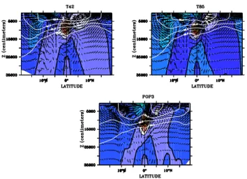
In this context and pending further progress with model sensitivity experiments we hypothesize that mean poleward transport in the vicinity of the WA continental slope arises from

The concentrations of sil- icate in the three largest river estuaries (Amazon, Congo and Orinoco) were similar to those measured in the smaller river systems (Niger, São

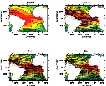
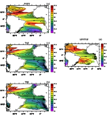
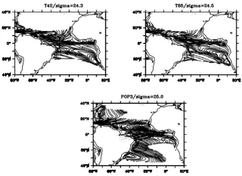
This study uses a set of regional simulations based on the ocean model NEMO to quantify the influence of the Amazon runoff on sea level in the Tropical Atlantic Ocean.. The model

The equatorial upwelling is also a productive region with a main phytoplankton bloom in July–August, when the Atlantic cold tongue is most developed, and a secondary

The tropical Atlantic observing system is motivated by goals to understand and better predict phenomena such as tropical Atlantic interannual to decadal variability and climate

ةيبرعلا تاصخللما v inCEnT r ondoT 88CL681+94CL331 بيبل خيشلا - يتحب اعـل ةدابع شقن تولم-لولأا-مهسلا-ةوقلا-ديدشلا لىإ ًانابرق مدقي وهو سوسينويد سوين شرع