HAL Id: hal-00728876
https://hal.inria.fr/hal-00728876
Submitted on 6 Sep 2012
HAL is a multi-disciplinary open access
archive for the deposit and dissemination of
sci-entific research documents, whether they are
pub-lished or not. The documents may come from
teaching and research institutions in France or
abroad, or from public or private research centers.
L’archive ouverte pluridisciplinaire HAL, est
destinée au dépôt et à la diffusion de documents
scientifiques de niveau recherche, publiés ou non,
émanant des établissements d’enseignement et de
recherche français ou étrangers, des laboratoires
publics ou privés.
Engineering a new algorithm for distributed shortest
paths on dynamic networks
Serafino Cicerone, Gianlorenzo d’Angelo, Gabriele Di Stefano, Daniele
Frigioni, Vinicio Maurizio
To cite this version:
Serafino Cicerone, Gianlorenzo d’Angelo, Gabriele Di Stefano, Daniele Frigioni, Vinicio Maurizio.
Engineering a new algorithm for distributed shortest paths on dynamic networks. Algorithmica,
Springer Verlag, 2012, �10.1007/s00453-012-9623-9�. �hal-00728876�
Engineering a new algorithm for distributed shortest
paths on dynamic networks
Serafino Cicerone · Gianlorenzo D’Angelo · Gabriele Di Stefano · Daniele Frigioni · Vinicio Maurizio
the date of receipt and acceptance should be inserted later
Abstract We study the problem of dynamically updating all-pairs shortest paths in a distributed network while edge update operations occur to the network. We consider the practical case of a dynamic network in which an edge update can occur while one or more other edge updates are under processing. A node of the network might be affected by a subset of these changes, thus being involved in the concurrent executions related to such changes.
In this paper, we provide a new algorithm for this problem, and experimen-tally compare its performance with respect to those of the most popular solu-tions in the literature: the classical distributed Bellman-Ford method, which is still used in real network and implemented in the RIP protocol, and DUAL, the Diffuse Update ALgorithm, which is part of CISCO’s widely used EIGRP protocol. As input to the algorithms, we used both real-world and artificial instances of the problem. The experiments performed show that the space oc-cupancy per node required by the new algorithm is smaller than that required by both Bellman-Ford and DUAL. In terms of messages, the new algorithm outperforms both Bellman-Ford and DUAL on the real-world topologies, while on artificial instances, the new algorithm sends a number of messages that is more than that of DUAL and much smaller than that of Bellman-Ford.
A preliminary version of this paper appeared in the proceedings of the 9th International Symposium on Experimental Algorithms (SEA2010) [9]
S. Cicerone · G. Di Stefano · D. Frigioni · V. Maurizio Department of Electrical and Information Engineering University of L’Aquila
Via G. Gronchi 18, I-67100 L’Aquila, Italy.
E-mail: [email protected], [email protected], [email protected], [email protected]
G. D’Angelo
MASCOTTE Project I3S(CNRS/UNSA)/INRIA
2004 Route Des Lucioles, BP 93, 06902 Sophia–Antipolis Cedex, France. E-mail: gian-lorenzo.d [email protected]
Keywords Shortest Paths, Distributed Networks, Dynamic Algorithms, Concurrent Update, Experimental Analysis.
1 Introduction
The problem of efficiently updating all-pairs shortest paths in a distributed network whose topology dynamically changes over the time, in the sense that link weights can be modified during the lifetime of the network, is considered crucial in today’s practical applications. Hence, it is very important to find efficient dynamic distributed algorithms for shortest paths. This problem has been widely studied in the literature, and the solutions found can be classified as distance-vector and link-state algorithms.
Distance-vector algorithms require that a node knows the distance from each of its neighbors to every destination and stores this information in a data structure usually called routing table. A node uses its own routing table to compute the distance and the next node in the shortest path to each destina-tion. Most of the distance-vector solutions for the distributed shortest paths problem proposed in the literature (e.g., see [8, 11, 13, 14, 16, 20, 21]) rely on the classical Distributed Bellman-Ford method (DBF from now on), originally introduced in the Arpanet [17], which is still used in real networks and imple-mented in the RIP protocol. DBF has been shown to converge to the correct distances if the link weights stabilize and all cycles have positive lengths [6]. However, the convergence can be very slow (possibly infinite) due to the well-known count-to-infinity phenomenon also know as routing table looping. A loop is a path induced by the routing table entries, such that the path visits the same node more than once before reaching the intended destination. A node “counts to infinity” when it increments its distance to a destination until it reaches a predefined maximum distance value. Furthermore, if the nodes of the network are not synchronized, even though no change occurs in the net-work, the overall number of messages sent by DBF is exponential in the size of the network (e.g., see [5]).
Link-state algorithms, as for example the Open Shortest Path First (OSPF) protocol widely used in the Internet (e.g., see [18]), require that a node knows the entire network topology to compute its distance to any network destina-tion (usually running the centralized Dijkstra’s algorithm for shortest paths). Link-state algorithms are free of count-to-infinity, however each node needs to receive and store up-to-date information on the entire network topology after a change, thus requiring quadratic space per node. This is achieved by broadcasting each change of the network topology to all nodes [18, 23, 24] and by using a centralized dynamic algorithm for shortest paths as for example those in [12, 19].
If the topology of a dynamic network is represented as a weighted undi-rected graph, then the typical update operations on that network can be mod-eled as insertions and deletions of edges and edge weight changes (weight decrease and weight increase). When arbitrary sequences of the above
opera-tions are allowed, we refer to the fully dynamic problem; if only inseropera-tions and weight decrease (deletion and weight increase) operations are allowed, then we refer to the incremental (decremental ) problem. We are interested in the practical case of a dynamic network in which an edge change can occur while one or more other edge changes are under processing. A node (processor) v of the network might be affected by a subset of these changes. As a consequence, v could be involved in the concurrent executions related to such changes.
Many algorithms proposed in the literature for the dynamic distributed shortest paths problem are not able to concurrently update shortest paths as those in [11,16,20,21]. In particular, they work under the assumption that be-fore dealing with an edge operation, the algorithm for the previous operation has to be terminated. This is a limitation in real networks, where changes can occur in an unpredictable way. For example, the algorithm proposed in [11] to handle weight increase operations works in three phases, and each phase starts when the previous one is completed. In a concurrent scenario, a new edge update can stop one of these phase thus making the algorithm incorrect. Among the algorithms which are able to concurrently update shortest paths (see, e.g., [8,10,13,14,22]) the most interesting is DUAL (Diffuse Update AL-gorithm) [13], which is free of the count-to-infinity phenomenon, thus resulting an effective practical solution (it is in fact part of CISCO’s widely used EIGRP protocol).
An incremental and a decremental solution have been proposed in [10]. Such solutions cannot deal with fully dynamic sequences of edge weight changes and the decremental solution suffers of count-to-infinity. In this paper, we extend the decremental solution of [10] by providing a new concurrent and fully dynamic algorithm for the distributed shortest paths problem denoted as DUST(Distributed Update of Shortest paThs). DUST suffers of the count-to-infinity problem, but it has been designed to heuristically reduce the cases where this phenomenon occurs. If we denote as n the number of nodes in the network, as deg(v) the degree of a node v, and as maxdeg the maximum node degree, DUST requires the same worst-case space occupancy per node of both DBFand DUAL that is O(n · maxdeg). However, DBF and DUAL store, for each node v, a data structure whose size is proportional to n · deg(v). In fact, they store specific information on each neighbor u of v, as for example, the distance from u to any other node s. Instead, DUST simply stores at node v the distance from v to s and all possible alternative vias to s, and does not store any information regarding its neighbors. This means that the space required by DUST depends on the node degree only in the worst case, which indeed occurs very rarely. In most of the cases the space occupancy of DUST does not depend on the node degree. For these reasons, it is worth measuring the practical performance of DBF, DUAL, and DUST in various dynamic re-alistic and artificial scenarios, in terms of both the overall number of messages they send, and their space occupancy per node.
With this goal in mind and following an algorithm engineering approach, we implemented DBF, DUAL, and DUST in the OMNeT++ simulation environ-ment [1], an object-oriented modular discrete event network simulator which
is widely used in the literature. As input to the algorithms, we used both real-world and artificial instances of the problem. In detail, we used snapshots of the Internet graph provided by the CAIDA IPv4 topology dataset [15]. CAIDA (Cooperative Association for Internet Data Analysis) is an association which provides data and tools for the analysis of the Internet infrastructure. Then, we used random Internet-like topologies with a power-law node degree distri-bution, generated by the Barab´asi-Albert algorithm [2]. Power-law networks have been proven to model many real-world networks such as the Internet, the World Wide Web, citation graphs, and some social networks [3]. Finally, since both CAIDA graphs and Barab´asi-Albert graphs turn out to be very sparse, we also analyzed random dense graphs generated by the Erd˝os-R´enyi algorithm [7].
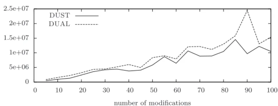
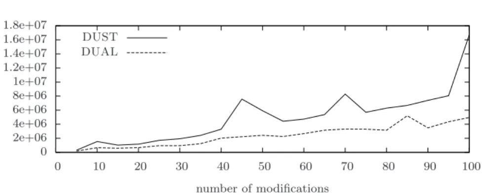
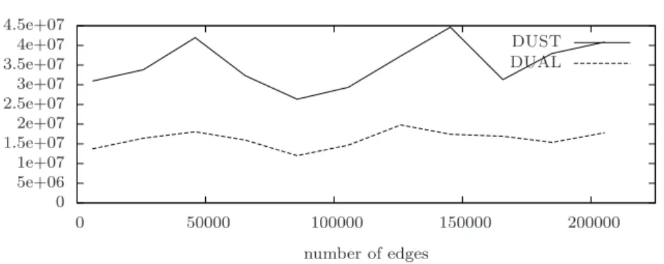
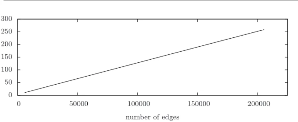
The experiments performed show that the space occupancy per node re-quired by DUST is much smaller than that rere-quired by both DBF and DUAL. In terms of number of messages sent, DUST outperforms both Bellman-Ford and DUAL on the Internet topologies provided by CAIDA. In Barab´asi-Albert artificial instances, DUST sends more messages than DUAL but fewer than Bellman-Ford. In the case of Erd˝os-R´enyi artificial instances, DUAL is still better than DUST in terms of number of messages, while we noticed a big increase in the space occupancy per node required by DUAL. In all our exper-iments, we observed that both DUAL (as expected) and DUST never counts to infinity, while in many cases DBF does. The last observation confirms the effectiveness of the heuristics implemented in DUST to reduce the cases where the count-to-infinity phenomenon occurs.
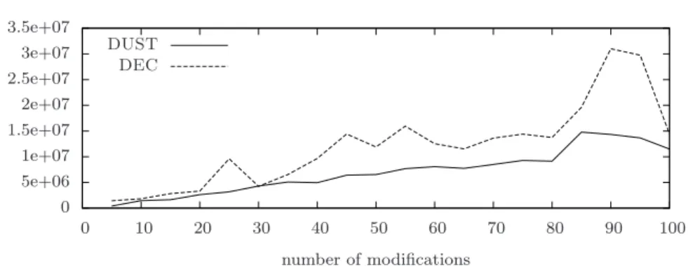
Finally, we compared DUST with the incremental and decremental so-lutions of [10], which are denoted from now on as INC and DEC, respec-tively. The comparison has been done separately, once for sequences of only weight increase operations and once for sequences of only weight decrease op-erations. While the space occupancy per node is always comparable, in term of number of messages sent, in the incremental case, DUST is slightly worse than INC and, in the decremental case, it is slightly better than DEC.
The paper is organized as follows. In Section 2 we describe the model and the notation used in the paper and the DBF and DUAL algorithms. In Section 3 we describe DUST. In Section 4 we give the correctness analysis of DUST. In Section 5 we report the results of our experimental study. Finally, in Section 6 we give some concluding remarks and outline possible future research directions. In the appendix, we give an example of execution of DBF, DUAL and DUST, useful to appreciate the differences among the algorithms.
2 Preliminaries
We consider a network made of processors linked through weighted communi-cation channels. Each processor can send messages only to its neighbors. We assume that messages are delivered to their destination within a finite delay but they might be delivered out of order. We consider an asynchronous
sys-tem, that is, a sender of a message does not wait for the receiver to be ready to receive the message. Finally, there is no shared memory among the nodes of the network.
Asynchronous model. We consider an asynchronous system based on that proposed in [4] and summarized below. The state of a processor v is the content of the data structure at processor v. The network state is the set of states of all the processors in the network plus the network topology and the channel weights. An event is the reception of a message by a processor or a change to the network state. When a processor p sends a message m to a processor q, m is stored in a buffer in q. When q reads m from its buffer and processes it, the event “reception of m” occurs. An execution is an alternate sequence (possibly infinite) of network states and events. A non negative integer number is associated to each event, the time at which that event occurs. The time is a global parameter and is not accessible to the processors of the network. The time must be non decreasing and must increase without bound if the execution is infinite. Events are ordered according to the time at which they occur. Several events can happen at the same time as long as they do not occur on the same processor. This implies that the times related to a single processor are strictly increasing.
Concurrent executions. We consider a dynamic network in which a change to the network topology or to the channel weights can occur while one or more other changes are under processing. A processor v could be affected by a subset of these changes. As a consequence, v could be involved in the executions related to such changes. Hence, according to the asynchronous model described above we need to define the notion of concurrent executions as follows. Let us consider an algorithm A that maintains some data structure on the processors of the network after a change to the network topology or to channel weights. Let ci and cj be two of such changes, we denote as: ti and tj the times at
which ci and cj occur, respectively; Ai and Aj the executions of A related to
ci and cj, respectively; and tAi the time when Ai terminates. If ti ≤ tj and
tAi ≥ tj, then Ai and Aj are concurrent, otherwise they are sequential.
Graph notation. We represent the network by an undirected weighted graph G = (V, E, w), where: V is a finite set of n nodes, one for each processor; E is a finite set of m edges, one for each communication channel; and w is a weight function w : E → R+∪ {∞}. An edge in E that links nodes u, v ∈ V is
denoted as u → v or (u, v). Given v ∈ V , N (v) denotes the set of neighbors of v and deg(v) the degree of v, which is the size of N (v). The maximum degree of the nodes in G is denoted by maxdeg. A path P in G between nodes u and v is denoted as P = u ; v. We define the length of P as the number of edges of P and denote it by ℓ(P ), and define the weight of P as the sum of the weights of the edges in P and denote it by weight(P ). A shortest path between nodes u and v is a path from u to v with the minimum weight. The distance from u to v is the weight of a shortest path from u to v, and is denoted as d(u, v). Given two nodes u, v ∈ V , the via from u to v is the
set of neighbors of u that belong to a shortest path from u to v. Formally: via(u, v) ≡ {z ∈ N (u) | d(u, v) = w(u, z) + d(z, v)}.
Given a graph G = (V, E, w), we suppose that a sequence C = (c1, c2, ..., ck)
of k operations is performed on edges (xi, yi) ∈ E, i ∈ {1, 2, ..., k}. The
oper-ation ci either inserts a new edge in G, or deletes an edge of G, or modifies
(either increases or decreases) the weight of an existing edge in G. We con-sider the case in which C is a sequence of weight increase and weight decrease operations, that is operation ci either increases or decreases the weight of edge
(xi, yi) by a quantity ǫi> 0, i ∈ {1, 2, ..., k}. The extension to delete and insert
operations, respectively, is straightforward: deleting an edge (x, y) is equiva-lent to increase w(x, y) to +∞, and inserting an edge (x, y) with weight α is equivalent to decrease w(x, y) from +∞ to α. Without loss of generality, we assume that operations in C = (c1, c2, ..., ck) occur at times t1≤ t2≤ ... ≤ tk,
respectively. Assuming G0 ≡ G, we denote as Gi the graph obtained by
ap-plying the operation cito Gi−1. We denote as di() and viai() the distance and
the via over Gi, 0 ≤ i ≤ k, respectively. Given a path P in G, we denote as
weighti(P ) the weight of P in Gi, 0 ≤ i ≤ k.
Distance vector algorithms. Here we describe the two most popular dis-tance vector algorithms known in the literature, the classical Bellman-Ford method (DBF) and the Diffuse Update Algorithm (DUAL).
DBFrequires each node v in the network to store the last estimated dis-tance towards any other node s ∈ V received from each neighbor u ∈ N (v), denoted as Dv[u, s]. In DBF, a node v updates its estimated distance to a node
s by simply executing the iteration Dv[v, s] := minu∈N(v){w(v, u) + Dv[u, s]}.
Like many distance vector algorithms, DBF suffers of the well-known count-to-infinity problem, which arises when a certain kind of link failure or weight increase operation occurs in the network. Figure 1 shows a classical topology where DBF counts to infinity. In particular, the left and right sides of such a figure show a graph G before and after a weight modification on edge (s, v). Figure 2 shows the steps required by DBF to update both the distance and
v s b a 100 1 1 v s b a 1 1 1 1 1
Fig. 1. A graph G before and after a weight modification on the edge (s, v).
the via to s for each node in G. In detail, when the weight of the edge (s, v) increases to 100, v updates its distance and via to s by setting Dv[v, s] to 3
and via to {a, b}. In fact, v knows that the distance from a (and b) to s is 2, while the weight of edge (v, s) is 100. Note that, v cannot know that the path
from a to s with weight 2 is that passing through edge (v, s) itself. Now, we concentrate on the operations performed by nodes a and b. When node a (b, respectively) performs the updating step, it finds out that its new via to s is b (a, respectively) and its new distance is 3. In fact, according to a’s information D[v, s] = 3 and D[b, s] = 2, therefore w(a, b) + D[b, s] < w(a, v) + D[v, s]. Subse-quent updating steps (but the last one) do not change the via to s of both a and b, but only the estimated distances. For each updating step the estimated distances increase by 1 (i.e., the weight of the edge (a, b)). The counting stops after a number of updating steps that depends on the new weight of the edge (s, v) and on the weight of edge (a, b). Note that, if edge (s, v) is deleted (i.e. his weight is set to ∞), the algorithm does not terminate.
... s b a 100 100 v 100 100 v s b a 101 100 101 100 s b a s b a 3 3 s b a 1 v v 3 3 v 3 3 2 2 2 2
Fig. 2. The sequence of recomputations of D[u, s] and VIA[u, s], u ∈ G, performed by DBF. The via to s is represented by a dotted arrow, while the number that lies close to the arrow represents the estimated distance.
DUAL requires, for each node v to maintain, for each destination s a set of neighbors called the feasible successor set F[v, s], and for each u ∈ N (v), the distance D[u, s] from u to s. F[v, s] is computed using a feasibility condition involving feasible distances from each node u in N (v) to s. In detail, node u is in F[v, s] if the estimated distance D[u, s] from u to s is smaller than the estimated distance D[v, s] from v to s. If the neighbor u, through which the distance to s is minimum, is in F[v, s], then u is chosen as successor to s. If F[v, s] does not include u, then v initiates a synchronous update procedure, known as diffuse computation. Node v sends queries to all its neighbors with its distance through the current successor by using message query. From this point onwards v does not change its successor to s until the diffusing computation terminates. When a neighbor u ∈ N (v) receives a queries, it updates F[u, s]. If u has a successor to s after such update, it replies to the query by sending message reply containing its own distance to s. Otherwise, u continues the diffuse computation: it sends out queries and waits for the replies from its neighbors before replying to v’s original query. When a node receives messages reply by all its neighbors, it updates its distance with the minimal value obtained by its neighbors and finishes the diffuse computation. At the end of a diffuse computation, a node sends message update containing the new computed distance to notify it to its neighbors. If there are concurrent updates, the node uses a finite state machine to process these multiple updates sequentially.
3 The new algorithm
In this Section we introduce DUST, our new solution for the concurrent up-date of distributed all-pairs shortest paths in dynamic networks. In detail, in Section 3.1, we define the data structure per node needed by DUST and give the pseudo-code of the algorithm; in Section 3.2, we outline the main ideas of the behavior of DUST by giving two examples of executions; in Section 3.3, we compare DUST with respect to DBF, DUAL, INC and DEC in terms of number of messages sent and space occupancy per node. The correctness of DUSTis given in Section 4.
3.1 Data structures and pseudo-code
Given G = (V, E, w), we assume that each node of G knows the identity of every other node of G, the identity of all its neighbors and the weights of the edges incident to it. The information on the shortest paths in G are stored in a data structure called routing table RT distributed over all nodes. Each node v maintains its own routing table RTv[·], that has one entry RTv[s], for each
s ∈ V . The entry RTv[s] consists of two fields:
– RTv[s].D, the estimated distance between nodes v and s in G;
– RTv[s].VIA ≡ {u ∈ N (v) | RTv[s].D = w(v, u) + RTu[s].D}, the estimated via from v to s.
For sake of simplicity, we write D[v, s] and VIA[v, s] instead of RTv[s].D and
RTv[s].VIA, respectively. As the data structures change over time, in what fol-lows we denote as Dt[v, s] and VIAt[v, s] the value of the data structures at
time t; we simply write D[v, s] and VIA[v, s] when the time is clear by the con-text. Given a destination s the set VIA[v, s] contains at most deg(v) elements. Hence, each node v requires O (n · deg(v)) space and the space complexity of DUSTis hence O (maxdeg · n) per node in the worst case.
Algorithm DUST is reported in Figure 3, 4 and 5, and is described in what follows with respect to a source s ∈ V . Before the algorithm starts, we assume that, for each v, s ∈ V and for each t < t1, Dt[v, s] and VIAt[v, s]
are correct, that is Dt[v, s] = d0(v, s) and VIAt[v, s] = via0(v, s). The
al-gorithm starts at each ti, i ∈ {1, 2, ..., k}. The event related to operation
ci on edge (xi, yi) is detected only by nodes xi and yi. As a consequence,
if ci is a weight increase (weight decrease) operation, xi sends the message
increase(xi, s) (decrease(xi, s, Dti[xi, s])) to yi and yi sends the increase(yi, s)
(decrease(yi, s, Dti[yi, s])) message to xi, for each s ∈ V . Note that message
decrease includes information about the distance from yi to s, while message
increase does not. In the case of a weight increase, in fact, such distance will be possibly obtained by xi in the subsequent rebuild-table phase (see the
following description).
If a node v receives the message decrease(u, s, D[u, s]), then it performs Procedure Decrease in Figure 3. Basically, Decrease performs a relaxation
Event: node v receives the message decrease(u, s, D[u, s]) from u Procedure Decrease
1. ifw(v, u) + D[u, s] < D[v, s] then 2. begin Lines 2-7: phase improve-table
3. D[v, s] := w(v, u) + D[u, s] 4. VIA[v, s] := {u} 5. for eachvi∈ N (v) do 6. send decrease(v, s, D[v, s]) to vi 7. end 8. else 9. if D[v, s] = w(v, u) + D[u, s] then
10. VIA[v, s] := VIA[v, s] ∪ {u} Line 10: phase extend-via
Fig. 3.
Event: node v receives the message increase(u, s) from u Procedure Increase
1. ifu∈ VIA[v, s] then 2. begin
3. VIA[v, s] := VIA[v, s] \ {u} Line 3: phase reduce-via
4. if VIA[v, s] ≡ ∅ then
5. begin Lines 5-17: phase rebuild-table
6. old distance:= D[v, s] 7. for eachvi∈ N (v) do
8. receive D[vi, s] by sending get-dist(v, s) to vi
9. D[v, s] := min vi∈N(v) {w(v, vi) + D[vi, s]} 10. VIA[v, s] := {vi∈ N (v)|w(v, vi) + D[vi, s] = D[v, s]} 11. for eachvi∈ N (v) do 12. begin
13. if D[v, s] > old distance then 14. send increase(v, s) to vi 15. send decrease(v, s, D[v, s]) to vi crh2 16. end 17. end 18. end Fig. 4.
of edge (u, v). In particular, if w(v, u) + D[u, s] < D[v, s] (Line 1), then v needs to update its estimated distance to s. To this aim, v performs phase improve-table, that updates D[v, s] and VIA[v, s] (Lines 3–4), and propagates the updated values to the nodes in N (v) (Line 6). Otherwise, if w(v, u) + D[u, s] = D[v, s] (Line 9), then u is a new estimated via for v wrt destination s, and hence v performs phase extend-via, that simply adds u to VIA[v, s] (Line 10).
If a node v receives the message increase(u, s), then it performs Procedure Increasein Figure 4. While performing Increase, v simply checks whether the message comes from a node in VIA[v, s] (Line 1). In the affirmative case, v needs to remove u from VIA[v, s]. To this aim, v performs phase reduce-via (Line 3). As a consequence of this deletion, VIA[v, s] may become empty. In
Event: node vireceives the message get-dist(v, s) from v
Procedure Send-Dist 1. if(VIA[vi, s] ≡ {v}) crt1
or(viis performing rebuild-table or improve-table wrt destination s) crt2
2. thensend ∞ to v crh1
3. elsesend D[vi, s] to v
Fig. 5.
this case, v performs phase rebuild-table, whose purpose is to compute the new estimated distance and via of v to s. To do this, v asks to each node vi∈ N (v) for its current estimated distance, by sending message get-dist(v, s)
to vi (Lines 7–8). When vi receives message get-dist(v, s) by v, it performs
Procedure Send-Dist in Figure 5. While performing Send-Dist, vi basically
sends D[vi, s] to v, unless one of the following two conditions holds:
1. VIA[vi, s] ≡ {v};
2. vi is performing rebuild-table or improve-table wrt destination s.
The test of these two conditions is part of our strategy to reduce the cases in which the count-to-infinity phenomenon appears. The test is performed at Line 1 of Send-Dist, where the conditions are labeled as crt1 and crt2,
respectively (the acronym stands for Count Reducing Test). If crt1 or crt2
are true, then vi sends ∞ to v. This action is performed at Line 2, and is
labeled as crh1 (the acronym stands for Count Reducing Heuristic). More
details on the strategy for the reduction of the count-to-infinity phenomenon are given in Section 3.3.
Once node v has received the answers to the get-dist messages by all its neighbors, it computes the new estimated distance and via to s (Lines 9–10). Now, if the estimated distance has been increased, v sends an increase message to its neighbors (Line 14). In any case, v sends to its neighbors the message decrease (Line 15), to communicate them D[v, s]. This action, that we call crh2, is also part of our strategy to reduce the count-to-infinity phenomenon. In fact, at some point, as a consequence of crh1, v could have sent ∞ to a
neighbor vj. Then, vjreceives the message sent by v at Line 15, and it performs
Procedure Decrease to check whether D[v, s] can determine an improvement to the value of D[vj, s].
3.2 Behavior of DUST
In what follows, we describe the behavior of DUST by giving two examples which focus on the steps performed by DUST when a sequence of only weight decrease or only weight increase operations occur. The aim of the first example is to show how procedure Decrease behaves, while the aim of the second ex-ample is to show how procedure Increase behaves and how the count preven-tion heuristics work. The steps performed by DUST when sequences of mixed
s u1 v viai(v, s) via j(v, s) ≡ viak(v, s) z3 z1 z2 u2 yj xj yi xi viaj(y j, s) ≡ viak(yj, s) viai(y i, s) ≡ viak(yi, s)
Fig. 6. Scenario for Case 1: only shortest paths from v to s in Gkare represented.
increase/decrease operations occur are a combination of those performed in the previous two cases.
In general, given a pair of nodes s, v ∈ V , at the end of the update sequence C = (c1, c2, ..., ck), that is at time tk, three cases may arise:
Case 1. The distance from v to s decreases, that is d0(v, s) > dk(v, s);
Case 2. The distance from v to s increases, that is d0(v, s) < dk(v, s);
Case 3. The distance from v to s does not change, that is d0(v, s) = dk(v, s).
Notice that, in each of the above cases, the distance between v and s can change (increase or decrease) many times between t0 and tk. We analyze the
three cases separately.
Case 1. d0(v, s) > dk(v, s). A possible scenario for the shortest paths from v
to s in Gk is shown in Figure 6, where the edges are represented as straight
lines while the paths are represented as curves. There are two weight decrease operations ci and cj, occurring at times ti and tj, ti < tj, that decrease the
weights of edges (xi, yi) and (xj, yj), respectively. As a consequence of these
operations, the distance from v to s decreases and the edges (xi, yi) and (xj, yj)
belong to the shortest paths from v to s in Gj. Here, we assume that c i and
cj are the only operations in C that affect the shortest paths from v to s. This
implies that viaj(v, s) ≡ viak(v, s) and di(v, s) = dj(v, s) = dk(v, s). In detail,
the shortest path from v to s in Gi is the path P
i = v → u1; yi → xi; s
and viai(v, s) ≡ {u
1}, while the shortest paths from v to s in Gj are the paths
Pi and Pj = v → u2 ; yj → xj ; s, and viaj(v, s) ≡ viak(v, s) ≡ {u1, u2}.
We show that the algorithm starts by updating the routing table of nodes yi
and yj, and then it updates the routing tables of the nodes in the sub-paths
When, at time ti, the weight decrease operation ci occurs, xi and yi send
their estimated distances to each other. When xireceives decrease(yi, s, Dti[yi, s])
by yi, it executes procedure Decrease in Figure 3, which first checks whether
it is necessary to start the algorithm (see Line 1). In the affirmative case, xi
updates D[xi, s] and VIA[xi, s] (see Lines 3–4) at a certain time t and sends the
message decrease(xi, s, Dt[xi, s]) to its neighbors (Line 6). The behavior of yi
(when yi receives the message decrease(xi, s, Dti[xi, s])) is symmetric. At most
one between xi and yi will propagate the decrease messages. In fact, if we
assume, without loss of generality, that Dti[xi, s] ≤ Dti[yi, s], then the test
per-formed by xiat Line 1 of Procedure Decrease is false. Thus, xidoes not need
to propagate the decrease message to its neighbors. Conversely, under the same assumptions, yi may improve its distance from s. In this case yi updates its
routing table at a certain time t and sends the message decrease(yi, s, Dt[yi, s])
to its neighbors. If we assume that Dtj[xj, s] ≤ Dtj[yj, s], the behavior of nodes
xj and yj at time tj is analogous to that of nodes xi and yi at time ti.
The decrease messages sent by yi (yj respectively) will update the values
of D[u, s] and VIA[u, s], for each node u in the subpath from yi (yj
respec-tively) to v of Pi (Pj respectively). Let us denote as mi and mj the decrease
messages received by v, and propagated along paths Pi and Pj respectively.
Further, let us denote as tmi and tmj the time when v receives mi and mj
respectively. Note that, in an asynchronous system, even if ti < tj, nothing
is known about the ordering of tmi and tmj. Let us assume that tmi < tmj,
the case where tmi > tmj is symmetric. When, at time tmi, v receives mi,
it performs improve-table phase of procedure Decrease and then, it up-dates D[v, s] and VIA[v, s] by setting D[v, s] = w(u, v) + di(u, s) = dk(v, s)
and VIA[v, s] ≡ {u1} ≡ viai(v, s). At time tmj, v receives mj and performs
extend-viaphase of procedure Decrease and then, it adds u2 to VIA[v, s] setting VIA[v, s] ≡ {u1, u2} ≡ viaj(v, s) ≡ viak(v, s). Finally, v sends the
message decrease(v, s, Dk[v, s]) to nodes in N (v). At this point, node v has
cor-rectly computed its current distance and via to s, and it has propagated this information to its neighbors.
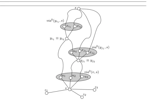
Case 2. d0(v, s) < dk(v, s). A possible scenario for the shortest paths from
v to s in G0 is represented in Figure 7. In this figure, we consider only
weight increase operations that occur on edges (xi1, yi1), (xi2, yi2), (xj1, yj1)
and (xj2, yj2). Note that, via
0(y
i1, s) ≡ {xi1, xi2} and via
0(y
j1, s) ≡ {u4, xj1, xj2}.
Since d0(v, s) < dk(v, s), each shortest path from v to s in G0 contains
an edge that has been increased by a weight increase operation. Moreover, there exist nodes yisuch that, for each xi∈ via0(yj1, s), edge (xi, yi) has been
increased. We call the set of such nodes Ys. For example, in the scenario of
Figure 7, Ys≡ {yi1} ≡ {yi2}.
In order to update its estimated distance and via to s, node v has to perform Procedure Increase. In particular, v has to perform reduce-via phase to remove from VIA[v, s] nodes that no longer belong to via(v, s). Moreover, if VIA[v, s] becomes empty, v has to perform rebuild-table phase to update its routing table and propagate the increase messages. In what follows we describe
yj1≡ yj2 xj2 u4 xj1 via0(y j1, s) u1 v z1 z3 z2 u2 u3 via0(v, s) s xi1 xi2 via0(y i1, s) yi1 ≡ yi2
Fig. 7. Scenario for Case 2: only shortest paths from v to s in G0are represented.
how nodes that increase their distance to s at time tk perform Procedure
Increase. First, (I) we show that nodes in Ys starts the updating phase by performing rebuild-table phase; then, (II) we show that node v is reached by the algorithm and it also performs rebuild-table phase; finally, (III) we show how v updates its routing table.
(I) For each i ∈ {1, 2, . . . , k}, such that yi∈ Ys, xi∈ via0(yi, s) and ci is a
weight increase operation, at time ti, nodes xiand yisend an increase message
to each other1. Each time that yi receives an increase message m, it removes
from VIA[yi, s] the node of via0(yi, s) that sent m (see phase reduce-via).
Hence, if t∅(yi, s) is the time when yi has received all the increase messages
coming from all the nodes in via0(y
i, s), then VIAt∅(yi,s)[yi, s] ≡ ∅. At time
t∅(yi, s), yi performs test at Line 4 of Procedure Increase, and the test
re-turns true. Hence, yiperforms rebuild-table phase which updates the
rout-ing table of yi and propagates the increase messages. More details on this
procedure are discussed later when we analyze the behavior of a generic node v. For example, in Figure 7, node yi1 sends an increase message to each node
in N (yi1) and hence, to neighbors of yi1 in the shortest paths from v to s in
G0that contain y i1.
(II) It can been shown by induction that each node in the shortest paths from yi1 to v and from yj1 to v has the same behavior of yi1, that is it
per-forms rebuild-table phase and sends increase messages to its neighbors. It 1 If the operation on edge (x
i, yi) is a delete operation, then yi(xi, respectively) cannot
receive any message by xi(yi). In this case, yi(xi) simulates the reception of the increase
follows that node v is eventually reached by increase messages sent by nodes in via0(v, s).
(III) Now we can analyze in detail the execution of rebuild-table phase by a generic node v at a certain time t. In order to update D[v, s] and VIA[v, s], v needs to know the estimated distances to s of each node in N (v), that is, Dt[vi, s], for each vi∈ N (v). In Figure 7, node v needs the estimated distance of each ziand uj, i, j ∈ {1, 2, 3}. To this aim, v sends the message get-dist(v, s)
to vi, for each vi ∈ N (v) (Line 8 of Procedure Increase). When, at a time tvi,
vi receives get-dist(v, s), it performs Procedure Send-Dist. Note that, in our
model, multiple increase and decrease messages on a single node are processed one by one, while get-dist messages are processed immediately. To analyze the behavior of nodes in N (v) when they receive get-dist messages, let us assume that, in the scenario of Figure 7, the following conditions hold:
– Node z1 satisfies crt1, that is at time tz1, VIAtz1[z1, s] ≡ {v};
– Node z2satisfies crt2, that is at time tz2, z2is performing rebuild-table
phase or improve-table phase wrt destination s.
Under these hypothesis, the answer to get-dist(v, s) messages of nodes z1 and
z2 is ∞, due to the execution of crh1, while we can assume that nodes u1,
u2, u3 and z3 answer with their current estimated distances to s. By using
the collected information, v updates D[v, s] and VIA[v, s] at Lines 9 and 10, re-spectively. Since z1and z2sent ∞ as their estimated distance to s, v does not
consider such nodes as possible elements of VIA[v, s]. Node z2 will eventually
send its current estimated distance to v as a decrease message by performing crh2. Moreover, at a certain time ¯t, node z1 will receive an increase message sent by v at the end of rebuild-table phase. If z1does not send further
mes-sages to nodes in N (z1), then VIA¯t[z1, s] ≡ VIAtz1[z1, s] ≡ {v}, and hence z1
will perform rebuild-table phase and then it will send a decrease message to v containing the current estimated distance from z1 to s, by performing
crh2. At this point, node v has received all the information needed to cor-rectly compute its current distance and via to s, and to propagate them to its neighbors.
Case 3. d0(v, s) = dk(v, s). Two cases may occur:
1. if di−1(v, s) = di(v, s), for each i ∈ {1, 2, . . . , k}, then the shortest paths
from v to s in Gk are the same of G0, that is v never updates RT v[s].
2. If there exists i ∈ {1, 2, . . . , k} such that di−1(v, s) 6= di(v, s), then there
ex-ists j ∈ {1, 2, . . . , k} such that if di−1(v, s) < di(v, s) (di−1(v, s) > di(v, s),
respectively), then dj−1(v, s) > dj(v, s) (dj−1(v, s) < dj(v, s),
respec-tively). In these cases, the algorithm propagates messages decrease and increase as in Cases 1 and 2.
In any case, v has correctly stored its current distance and via to s, and, possibly, it has propagated this information to its neighbors.
3.3 Comparison to existing algorithms
In what follows, we compare DUST with DBF, DUAL, INC and DEC in terms of number of messages sent and space occupancy per node.
Like many other distance vector algorithms, both DBF and DUST suffer of the count-to-infinity problem and hence the number of messages sent cannot be asymptotically bounded by a function of the size of the graph. However, DUST has been designed to heuristically reduce the number of cases where it counts to infinity. In fact, let us consider again the example of Figure 1 where DBF counts to infinity. In Figure 8 we show the few steps required by algorithm DUST to update both the distance and the via to s for each node in the graph G of Figure 1. When s and v detect the weight change on
v s b a 2 1 2 v s b a 2 100 2 v s b a 101 100 101
Fig. 8. The sequence of recomputations of D[u, s] and VIA[u, s], u ∈ G, performed by DUST.
edge (s, v), they perform Procedure Increase with respect to source s. In particular, s does not perform rebuild-table phase as VIA[s, s] = ∅, while v does. When v gets the estimated distances to s from its neighbors (Line 8 of Procedure Increase), it receives ∞ from both a and b. This is due to the fact that since test crt1 returns true, a and b apply heuristic crh1. At the end
of these execution, v correctly updates its routing table and sends messages increase and decrease to each neighbor. It is easy to verify that, when s receives the decrease and increase messages from v, it does not perform any local data modification. In contrast, both a and b perform Procedure Increase when they receive the increase message from v. In this case, a and b send ∞ (as their estimated distance to s) to each other in response to the get-dist message. This is due to the fact that the algorithm applies again crh1but, in this case,
crh1 is due to test crt2, which returns true. Hence, both a and b correctly update their routing tables by using messages sent by v. Subsequent messages sent by a and b do not produce further local data modification.
In the previous example, there are nodes that apply action crh2. However,
this action is never effective since the conditions of Lines 1 and 9 of Decrease are always false. In what follows, we describe how to modify the graph G in Figure 1 in order to fully appreciate our strategy to reduce the count-to-infinity phenomenon. Consider a graph G′ obtained from G by adding the edge (s, a)
with w(s, a) = 98. In this case, when a and b receive the increase message from v, they update their routing tables as follows: D[a, s] = 98 and D[b, s] = 101. At this point node a performs crh2 by sending a decrease message to b and to
v. When b and v perform Procedure Decrease, they set D[b, s] = D[v, s] = 99 and VIA[b, s] = VIA[v, s] = {a}. Notice that, DBF still counts to infinity on G′,
but, in this case, the counting stops after a number of updating that depends on the weight of the edge (s, a).
To conclude our comparison of DUST and DBF, we give an example where they both DBF and DUST count to infinity. Let us consider the graph of Figure 1 where the weight of edge (a, v) is set to 2. At time t0, D[a, s] = 3
and VIA[a, s] = {v, b}. Now, the weight of edge (s, v) increases to 100. When v executes rebuild-table phase, it receives ∞ by b but it receives 3 from a and sets D[v, s] = 5 and VIA[v, s] = {a}. Then v sends increase messages to a and b. Let us assume that the message sent to a is received before that sent to b. Then, when a receives such message, it performs reduce-via and sets VIA[a, s] = {v, b} \ {v} = {b}. When b receives the increase message by v it performs rebuild-table and sets VIA[b, s] = {v}. In the resulting configuration VIA[·, s] forms a loop, the count-to-infinity phenomenon occurs and the number of messages sent depends on the new weight on the edge (s, v). Regarding the comparison with DUAL, as already observed, DUAL and DUST asymptotically requires the same space per node in the worst case, that is O(n · maxdeg). However, in what follows we observe that in practice the memory requirement of DUST is smaller than that of DUAL. DUAL requires a node v to store, for each destination s, the estimated distance D[u, s] from each of its neighbors u, hence the space requirement of dual is exactly O(n · deg(v)). DUST only needs the estimated distance of v to s and the set VIA[v, s]. In the worst case, VIA[v, s] can have deg(v) elements, but in practice this happens rarely (indeed, as we will experimentally show, it is not common to have more than one node in such set). It hence follows that the practical space requirements of DUST do not depend on the node degree.
In contrast to the space occupancy, the node degree affects the perfor-mances of DUST in terms of the number of messages sent. In fact, as DUST does not store the estimated distances of its neighbors, it needs to ask for them by sending get-dist message when they are needed. Hence, the number of get-dist messages sent by a node is proportional to the node degree. For this reason, in general DUAL sends a number of messages which is smaller than that of DUST. However, in real-world graphs the average node degree is small and then the number of get-dist messages sent is also small. In fact, we will experimentally show that in real-world graphs DUST sends less messages than DUAL.
Regarding the comparison with DEC and INC, we stress that such so-lutions are only incremental and decremental, respectively, and hence cannot cope with fully dynamic sequences of updates as the two algorithms use dif-ferent data structure. In particular, INC has an optimal space occupancy per node as it stores only the routing table and it has a message complexity that is a factor maxdeg far from the optimal one. Such good theoretical bound of INC are due to the hypothesis that only weight decrease operations are as-sumed to occur in the network. In fact, INC is able to discard many messages thanks to a filtering condition which cannot be used in case of weight increase
operations. DEC uses the same data structure of DUST and counts to in-finity. However, DUST, in addition to being fully dynamic, is able to reduce the cases where the count-to-infinity occurs in sequences of weight increase operations, thanks to heuristic crh2which is not used in DEC.
4 Correctness
In this section, we prove the correctness of DUST. Let G be a graph and C = (c1, c2, ..., ck) a sequence of weight increase and weight decrease operations
occurring on G at times t1≤ t2≤ ... ≤ tkand generating graphs G1, G2, . . . Gk,
respectively. We show that, for any pair of nodes v and s, there exists a time tF such that for each time t ≥ tF the routing table of v with respect to s is
that of Gk, formally:
Dt[v, s] = dk(v, s) and VIAt[v, s] ≡ viak(v, s).
Such statement is proven in Theorem 1, the following lemmata are needed for the proof.
Lemma 1 Given v, s in G such that d0(v, s) < dk(v, s), there exists a node y
such that, for each x ∈ via0(y, s), w(x, y) has been increased by an operation in C, and d0(y, s) < dk(y, s).
Proof. By contradiction, let us suppose that, for each y ∈ {y1, y2, . . . , yk},
either there exists z ∈ via0(y, s) such that w(z, y) has not been increased by any weight increase operation, or d0(y, s) ≥ dk(y, s). This implies that nodes
of G can only decrease the distance to s as a consequence of the weight changes c1, c2, ..., ck. Hence, d0(v, s) ≥ dk(v, s), which is a contradiction. 2
Let Ysbe the set of nodes y satisfying Lemma 1 with respect to destination s.
Lemma 2 Given v, s in G such that d0(v, s) < dk(v, s), there exists y ∈ Y s
and a time t∅(y, s) such that VIAt∅(y,s)[y, s] ≡ ∅.
Proof. By contradiction, let us suppose that, for each node y in Ysand for each
time t, VIAt[y, s] 6≡ ∅. Let y be a node in Ys. Each node x in via0(y, s) sends
an increase message to y as a consequence of the weight increase operation on edge (x, y). When y receives this message, it performs the reduce-via phase of Procedure Increase and deletes x from VIA[y, s]. Hence, there exists a time when VIA[y, s] contains only nodes that have been added as a consequence of other increase or decrease messages received by y.
Furthermore, since VIA[y, s] is never empty, the condition in line 4 of pro-cedure Increase is always false and y never performs rebuild-table phase. This implies that for each pair of times t′, t′′ such that t′ < t′′, D
t′[y, s] ≥
Dt′′[y, s] (that is, D[y, s] decreases over time) and that each node u in VIA[y, s]
have been added to such set as a consequence of a decrease message m = decrease(u, s, Dtu[u, s]) sent by u to y. If ¯ti0 > tu is the time when y receives
m, we have Dt¯i0[y, s] ≥ w(y, u) + Dtu[u, s]. Let P be the path from y to s
con-taining u whose estimated weight is w(y, u) + Dtu[u, s]. Since y received m, P
must contain an edge whose weight has been changed by an operation c ∈ C. If c is a weight decrease operation, then P must contain also an edge whose weight has been increased by another operation in C. In fact, since D[y, s] decreases over time, we have that d0(y, s) ≥ D
¯
ti0[y, s] ≥ w(y, u) + Dtu[u, s],
that is the estimated weight of P is smaller or equal to d0(y, s). But, since
by hypothesis d0(y, s) < dk(y, s), the actual weight of P in Gk is such that
weightk(P ) > d0(y, s). Hence, in any case, P contains an edge whose weight
has been increased by another operation in C, that is P has the following structure
P = y → u ; ¯y → ¯x ; s
where edge (¯x, ¯y) is the edge whose weight has been increased. Since d0(y, s) <
dk(y, s), then all paths having the following structure
P′= y ; ¯y ; s
where y ; ¯y is the subpath of P from y to ¯y, satisfy weightk(P′) > d0(y, s).
It follows that, d0(¯y, s) < dk(¯y, s). The set via0(¯y, s) consists of two disjoint
subsets, ¯X(¯y, s) ≡ {x | w(x, ¯y) has been increased by an operation in C} and ¯
U (¯y, s) ≡ via0(¯y, s) \ ¯X(¯y, s), where ¯X(¯y, s) 6≡ ∅, since ¯x ∈ ¯X. If ¯U (¯y, s) ≡ ∅, then ¯y ∈ Ys. If ¯U (¯y, s) 6≡ ∅, then, for each node ¯u ∈ ¯U (¯y, s), there exists a path
from ¯u to s that contains a node in Ys. In any case, there exists a path from
y to s having the following structure
P0= y → u ; yi1 → xi1 ; s
where edge (xi1, yi1) is an edge whose weight has been increased. Furthermore
yi1 ∈ Ys, hence the same arguments can be used to show that there exists a
path:
P1= yi1→ ui1 ; yi2→ xi2 ; s
where the edge (xi2, yi2) is involved in a weight increase operation, yi2 ∈ Ys
and D¯ti1[yi1, s] ≥ w(yi1, ui1) + Dtui1[ui1, s], tui1 < tyi1. In general, for each
yj ∈ Ysthere exists a path:
Pj= yj → uj ; yj+1→ xj+1; s
where the edge (xj+1, yj+1) is involved in a weight increase operation, yj+1∈
Ys and Dtj[yj, s] ≥ w(yj, uj) + Dtuj[uj, s], tuj < tj. That is, since |Ys| < ∞,
there exists a cycle:
y → u ; yi1→ ui1 ; yi2→ ui2 ; ... ; yih → uih ; y
such that:
D¯
ti0[y, s] ≥ w(y, u) + Dtu[u, s] > Dtu[u, s] ≥
D¯t
... D¯t ih[yih, s] ≥ w(yih, uih) + Dtuih[uih, s] > Dtuih[uih, s] ≥ D¯ t′ i0[y, s], where ¯ti0 > tu > ¯ti1 > tui1... > ¯tih > tuih > ¯t ′
i0, that is D¯ti0[y, s] > Dt¯′i0[y, s]
with ¯ti0 > ¯t
′
i0 that is a contradiction. Hence there exists y ∈ Ys and a time
t∅(y, s) such that VIAt∅(y,s)[y, s] ≡ ∅. 2
Let us denote as Y′
s⊆ Ysthe set of nodes satisfying Lemma 2 with respect
to destination s. The next Lemma states that condition in Line 13 of Procedure Increaseis true for each y in Y′
s, and hence that y sends increase messages
to nodes in N (y).
Lemma 3 Given v, s in G such that d0(v, s) < dk(v, s), for each y ∈ Y′ s, y
sends an increase message to each node in N (y). Proof. Each node y in Y′
s performs rebuild-table phase at least once at time
t∅(y, s). By contradiction, let us suppose that each execution of rebuild-table
phase does not send any increase message, that is the condition in line 13 of procedure Increase is always false, for each y ∈ Y′
s. Hence, for each y ∈ Y ′ s
and for each t∅(y, s), if we denote as t′y the time when y performs line 9 of
procedure Increase, there exists a node u in N (y) and a time tu < t′y such
that:
Dt′
y[y, s] = w(y, u) + Dtu[u, s] ≤ Dt∅(y,s)[y, s].
Let Pube the path from y to s containing u whose estimated weight is w(y, u)+
Dt
u[u, s]. The same arguments used in the proof of Lemma 2 can be used
to prove that Pu contains an edge whose weight has been increased by an
operation in C and to derive a contradiction. 2
The next Lemma states that each node v such that d0(v, s) < dk(v, s) has
the same behavior of nodes in Y′
s that is, v performs rebuild-table phase
and sends increase message to each node in N (v).
Lemma 4 Given v, s in G such that d0(v, s) < dk(v, s), v performs rebuild-table
phase wrt source s and it sends an increase message to each node in N (v). Proof. We denote as:
Ps(v) = {P = v ; y | y ∈ Ys′∧ ∃ P′= v ; s : P ⊆ P′}
Ls(v) = max{ℓ(P ) | P ∈ Ps(v)}
the proof is by induction on Ls(v).
Inductive basis (Ls(v) = 0): a node v is such that Ls(v) = 0 and d0(v, s) <
dk(v, s) if and only if v ∈ Y′
s. By Lemma 2, v performs rebuild-table phase
and by Lemma 3, it sends an increase message to each node in N (v).
Inductive step: the inductive hypothesis is: each node v such that Ls(v) ≤ l−1
and d0(v, s) < dk(v, s) performs rebuild-table phase and sends and increase
Let v be a node such that Ls(v) = l and d0(v, s) < dk(v, s) and u be a
node in N (v) such that: Dt
v[v, s] = w(v, u) + Dtu[u, s]
u ∈ VIAtv[v, s]
at certain times tv and tu such that tu< tv.
Two cases may occur:
– d0(u, s) < dk(u, s): by inductive hypothesis, u sends an increase message
to v.
– d0(u, s) ≥ dk(u, s): let P
s(v, u, tv) be the set of estimated shortest paths
from v to s via u at time tv. Since d0(v, s) < dk(v, s), each path P in
Ps(v, u, tv) contains a node yP ∈ Ys. For each P ∈ Ps(v, u, tv), yP is such
that Ls(yP) ≤ l − 1, then yP sends an increase message to each node in
N (yP). Thus the message is propagated in each path in Ps(v, u, tv). Hence
u sends an increase message to v.
In any case, each node in VIAtv[v, s] sends an increase message to v and then
there exists a time t when VIAt[v, s] ≡ ∅ and v performs rebuild-table phase.
The same arguments can be used to show that v sends an increase message
to each node in N (v). 2
In the remainder we will use the following further notation for each pair of nodes v and s:
– Exel(v, s) denotes the last local execution by v of phases rebuild-table
or improve-table with respect to s;
– tl(v, s) is equal to t1if v never performs neither rebuild-table phase nor
improve-tablephase, otherwise, tl(v, s) is the time when Exel(v, s) per-forms Lines 9 and 10 of Procedure Increase or Lines 3 and 4 of procedure Decrease.
– t′
l(v, s) is the time when v modify D[v, s] for the last time, tl(v, s) ≥ t′l(v, s).
Lemma 5 For each pair of nodes v and s and for any time t ≥ t′ l(v, s),
Dt[v, s] ≥ dk(v, s).
Proof. Two cases may occur:
1. v never updates D[v, s]. For any time t, we have: Dt[v, s] = d0(v, s).
As v never updates D[v, s], it never performs rebuild-table and it never sends increase messages, hence, by Lemma 4, d0(v, s) ≥ dk(v, s). Then, for
each time t:
2. v updates D[v, s] at least once. By contradiction, let us suppose that v is the first node failing to update its routing table and let tv≥ t′l(v, s) be the
smallest time such that Dt
v[v, s] < d
k(v, s). (1)
For each z ∈ VIAtv[v, s], Dtv[v, s] = w(v, z) + Dtz[z, s], tz< tv.
If there exists a node z ∈ VIAtv[v, s] such that tz ≥ t
′
l(z, s), since v is
the first node to fail, then Dtz[z, s] ≥ d
k(z, s). Thus D
tv[v, s] = w(v, z) +
Dt
z[z, s] ≥ w(v, z) + d
k(z, s) ≥ dk(v, s), a contradiction with respect to
Equation 1. Hence, in what follows, we assume that tz < t′l(z, s) for each
z ∈ VIAtv[v, s].
If there exists a node z ∈ VIAtv[v, s] that never updates D[z, s], then, by
Case 1, we have that Dtz[z, s] ≥ d
k(z, s) and then D
tv[v, s] ≥ d
k(v, s),
a contradiction with respect to Equation 1. Hence, in what follows, we assume that z ∈ VIAtv[v, s] updates D[z, s] at least once.
When a node z ∈ VIAtv[v, s] updates D[z, s] at time t
′
l(z, s) > tz, it sends
a decrease message m. When v receives m at time tm(z, v), it performs
Procedure Decrease. If, at time t′
l(z, s), z decreases the value of D[z, s],
then, v performs improve-table as a consequence of m and modifies D[v, s] after the time t′
l(v, s), a contradiction with respect to the definition of
t′l(v, s). In fact, since tv≥ t′l(v, s), after tv, Dt[v, s] does not change and then
Dt[v, s] = w(v, z)+Dt
z[z, s] for each t ≥ tv. Hence, since D[z, s] as decreased,
at time tm(z, v), the condition at Line 1 of Procedure Decrease is true
and v performs improve-table as a consequence of m and modifies D[v, s] after the time t′
l(v, s). Hence, let us assume that each node z ∈ VIAtv[v, s],
at time t′
l(z, s), increases the value of D[z, s].
Under this hypothesis, each node z ∈ VIAtv[v, s] also sends an increase
message m′ that is received by v at time t
m′(z, v). In fact, the value of
D[z, s] can increase only during rebuild-table and, if D[z, s] increases, the condition at Line 13 of Procedure Increase is true.
Since tv ≥ t′l(v, s), after tv, v can only perform phases rebuild-table,
reduce-via and extend-via. Let Ext(v, s) be the set of nodes added to VIA[v, s] after tv as a consequence of an rebuild-table or a extend-via phase performed by v. We can assume that each node z in Ext(v, s) fulfills the same properties of nodes in VIAtv[v, s], that is:
(a) tz< t′l(z, s),
(b) z updates D[z, s] at least once, (c) at time t′
l(z, s), z increases the value of D[z, s] and then it sends an
increase message m′ that is received by v at time t
m′(z, v).
Let tmax= max{tm′(z, v) | z ∈ VIAt
v[v, s] ∪ Ext(v, s)}. Informally, tmax is
the time when v receives the last increase message from nodes in VIAtv[v, s]∪
Ext(v, s). It follows that, at time tmax, v performs Procedure Increase and
tests at Lines 1 and 4 return true. Then, v performs phase rebuild-table at time tmax > tv ≥ tl(v, s). Furthermore, since each z ∈ VIAtv[v, s] ∪
Ext(v, s) increases the value of D[z, s], v increases D[v, s] after the time t′
l(v, s), a contradiction with respect to the definition of t ′ l(v, s).
2 Corollary 1 For each pair of nodes v and s and for any time t ≥ tl(v, s),
Dt[v, s] ≥ dk(v, s).
Proof. Since tl(v, s) ≥ t′l(v, s), the statement follows directly by Lemma 5 2
Remark 1 Let v be a node in V and z be a node in N (v). If there exists a pair of times t′, t′′ such that:
– t′≤ t′′;
– for each tz, t′≤ tz≤ t′′, Dtz[z, s] = ¯d where ¯d is a certain real value;
– at time tv, t′≤ tv ≤ t′′, Dtv[v, s] ≤ w(v, z) + ¯d.
Then, for each time t, tv≤ t ≤ t′′, Dt[v, s] ≤ w(v, z) + ¯d.
Theorem 1 There exists tF such that, for each pair of nodes v, s ∈ V , and
for each time t ≥ tF,
Dt[v, s] = dk(v, s) and VIAt[v, s] ≡ viak(v, s).
Proof. The correctness of the algorithm is shown with respect to a fixed source s. The correctness for all pairs of nodes is a straightforward consequence. In fact, since procedures Decrease, Increase and Send-Dist always refer to the record of the routing table related to a single source, then two executions of the algorithm related to two different sources cannot access the same record of the routing table.
If the statement is true for nodes v and s, then we denote as tF(v, s) the
time when the statement occurs for v and s. If there exists tF(v, s) for each
v, s ∈ V , then tF = max
v∈V(tF(v, s)). Now we show that tF(v, s) exists for a
generic pair (v, s). We need the following definitions:
Ps(v) = {P = v ; s | P is a shortest path in Gk}
Ls(v) = max{ℓ(P ) | P ∈ Ps(v)}
the proof is by induction on Ls(v).
Inductive basis (Ls(v) = 0): the unique node such that Ls(v) = 0 is s. For any
time t ≤ t1, we have:
Dt[s, s] = d0(s, s) = 0 VIAt[s, s] ≡ via0(s, s) ≡ ∅.
If s never changes RTs[s], then tF(s, s) = t1. Hence we have to show that s
does not perform any of the following phases: improve-table, extend-via, reduce-viaand rebuild-table. Node s can perform:
– improve-tableor extend-via as a consequence of a decrease message; – reduce-viaand rebuild-table as a consequence of an increase message. Let tm be the time when s receives the first decrease or increase message m.
– if m = decrease(z, s, Dtz[z, s]), where z ∈ N (s) and tz < tm, then, since
Dt
m[s, s] = 0 and w(s, z) > 0, the condition in lines 1 and 9 of procedure
Decreaseare false. Thus v does not perform neither improve-table nor extend-viaphase.
– if m = increase(z, s), where z ∈ N (s), then, since VIAtm[s, s] ≡ ∅, the
condition in line 1 of procedure Increase is false. Thus v does not perform neither reduce-via nor rebuild-table phase.
In any case, s does not change RTs[s] then, if s receives further messages, the
same arguments can be used to prove the statement. Hence tF(s, s) = t1.
Inductive step: the inductive hypothesis is: each node v such that Ls(v) ≤ l−1
correctly assigns DtF(v,s)[v, s] and VIAtF(v,s)[v, s]. Let v be a node such that
Ls(v) = l. Each node u in viak(v, s) satisfy the inductive hypothesis.
Now we show that there exists a time tD(v, s) such that, for each t ≥ tD(v, s), Dt[v, s] = dk(v, s). We analyze different cases according to the behavior
of nodes in viak(v, s).
– If each node u in viak(v, s) does not send any message to v, then, it does
not perform rebuild-table and improve-table phases and then it never changes D[u, s]. Hence, by inductive hypothesis, for each time t, Dt[u, s] =
d0(u, s) = dk(u, s). Furthermore, since u does not change its distance to s,
we have d0(v, s) ≤ dk(v, s). Hence, at time t 1:
Dt
1[v, s] = d
0(v, s) ≤ dk(v, s) = w(v, u) + dk(u, s)
and, since, for each time t ≥ t1, Dt[u, s] does not change, by Remark 1, we
have:
Dt[v, s] ≤ w(v, u) + dk(u, s) = dk(v, s). Furthermore, by Corollary 1, for each t ≥ tl(v, s):
Dt[v, s] ≥ dk(v, s). Thus tD(v, s) = max{t1, tl(v, s)}.
– If at least a node in viak(v, s) sends a message to v, then, let u
1, u2, ..., uh
be the nodes in viak(v, s) that send a message to v. By inductive
hy-pothesis, each ui sends to v at least one of the messages: increase(ui, s)
or decrease(ui, s, dk(ui, s)). Let mui be the last of such messages sent by
ui and let m = increase(u, s) or m = decrease(u, s, dk(u, s)) be the first
message among mui, 1 ≤ i ≤ h, received by v.
When v receives m, it performs the procedure Increase or Decrease and, as a consequence, at time tmstores:
Dt
m[v, s] ≤ w(v, u) + d
k(u, s).
Since m is the last message sent by u, for each time t ≥ tm, Dt[u, s] does
not change and then, by Remark 1, we have:
Furthermore, by Corollary 1, for each t ≥ tl(v, s):
Dt[v, s] ≥ dk(v, s). Thus: tD(v, s) = max{tm, tl(v, s)}.
Now we show that there exists a time tVIA(v, s) such that, for each t ≥ tVIA(v, s), VIAt[v, s] ≡ viak(v, s).
Let u be a node in viak(v, s) and t
mu be the time when v receives the last
message mugiving a correct estimated distance from u to s or a time before t1
if u never updates D[u, s]. Now we analyze different cases according to tmu. For
each of such cases we show that u is added to VIA[v, s] and is never removed anymore.
– tmu > tl(v, s). We now show that mu = decrease(u, s, d
k(u, s)). By
con-tradiction, let us suppose that mu = increase(u, s). Then, since u sends
an increase message only if test at Line 13 of procedure Decrease is true, there exists a time ˜t such that, for each t, t1 ≤ ˜t ≤ t < tl(v, s),
Dt[u, s] < dk(u, s) and ˜t is the smallest time that fulfill this condition. For each of the following cases we obtain a contradiction:
– if ˜t < tl(v, s), then by Remark 1:
Dt
l(v,s)[v, s] ≤ w(v, u) + D˜t[u, s] < w(v, u) + dk(u, s) = dk(v, s)
that is a contradiction with respect to Corollary 1.
– If ˜t ≥ tl(v, s), then at time ˜t, u sends the message decrease(u, s, D˜t[u, s])
that is received by v at time ¯t > ˜t. At time ¯t, we have: D¯
t[v, s] = dk(v, s) = w(v, u) + dk(u, s) < w(v, u) + D˜t[u, s].
Hence the condition in line 1 of procedure Decrease is true and v performs improve-table phase at a time greater then tl(v, s) that is
a contradiction with respect to the definition of tl(v, s).
Hence, mu= decrease(u, s, dk(u, s)).
Since tmu > tl(v, s), then Dtmu[v, s] = d
k(v, s) = w(v, u) + dk(u, s). Hence,
when v receives mu, the condition in line 9 of procedure Decrease is true
and then v adds u to VIA[v, s] at time tu.
Since mu is the last message sent by u to v and, at time t > tu, v has
performed Exel(v, s), u will not be removed from VIA[v, s].
– tmu < tl(v, s). We now show that Exel(v, s) performs phase rebuild-table.
By Remark 1, we have that, for each t ≥ tmu,
Dt[v, s] ≤ w(v, u) + dk(u, s) = dk(v, s).
By contradiction, let us suppose that Exel(v, s) performs improve-table
as a consequence of a decrease message received at time ˜t ≥ tmu. Then the
condition at Line 1 of procedure Decrease is true and, at time tl(v, s), v
assigns a value of D[v, s] such that: Dt
l(v,s)[v, s] < D˜t[v, s] ≤ d
that is a contradiction with respect to Corollary 1. Hence Exel(v, s)
per-forms phase rebuild-table. Since tmu < tl(v, s), Dt¯[u, s] = d
k(u, s), where ¯t is the time when, during
Exel(v, s), v receives D[u, s] as an answer to the message get-dist(v, s) sent
to u. Hence v adds u to VIA[v, s] at time tu= tl(v, s).
Since mu is the last message sent by u to v and, at time t > tu, v has
performed Exel(v, s), u will not be removed from VIA[v, s].
– tmu = tl(v, s). Since two events cannot occur to the same processor at the
same time, we have tmu = tl(v, s) < t1 that is, neither u nor v changes
its distance estimate to s and u does not sends any message to v. Thus u ∈ via0(v, s) and v never removes u from VIA[v, s]. In this case we denote
tu= t1.
Thus for each time t ≥ max{tu| u ∈ viak(v, s)}, each node in viak(u, s) belongs
to VIAt[u, s].
There may exist a node z in N (v) \ viak(v, s) that belongs to VIA
t[u, s] for
a certain time t. Since z /∈ viak(v, s), then dk(v, s) < w(v, s) + dk(z, s). Hence
v added z to VIAt[v, s] as a consequence of an underestimated value of D[z, s].
By Corollary 1, at time tl(z, s), z will increase its estimated distance and send
to v an increase message mz= increase(z, s). As a consequence, v will perform
phase reduce-via at time tz. Thus:
tVIA(v, s) = max{{tu | u ∈ viak(v, s)} ∪ {tz | z ∈ N (v) \ viak(v, s)}}.
Hence for a generic node v we have: tF(v, s) = max{tD(v, s), tVIA(v, s)}. 2
5 Experimental analysis
In this section, we report the results of our experimental study on the per-formance of DUST against DBF, DUAL, INC and DEC. In detail, we first describe the implementation platform and the executed tests, and then we analyze the results of our study.
Experimental environment. The experiments have been carried out on a workstation equipped with a 2.66 GHz processor (Intel Core2 Duo E6700 Box) and 8Gb RAM. The experiments consist of simulations within the OMNeT++ environment, version 4.0p1 [1]. OMNeT++ is an object-oriented modular dis-crete event network simulator, useful to model protocols, communication net-works, multiprocessors and other distributed systems. An OMNeT++ model consists of hierarchically nested modules, that communicate through message passing. In our model, we defined a basic module node to represent a node in the network. A node v has a communication gate with each node in N (v). Each node can send messages to a destination node through a channel which is a module that connects gates of different nodes (both gate and channel are OMNeT++ predefined modules). A channel connects exactly two gates and represents an edge between two nodes. We associate two parameters per chan-nel: a weight and a delay. The former represents the weight of the edge in the graph, and the latter simulates a finite but not null transmission time.

![Fig. 2. The sequence of recomputations of D[u, s] and VIA[u, s], u ∈ G, performed by DBF](https://thumb-eu.123doks.com/thumbv2/123doknet/13577574.421730/8.918.111.613.371.482/fig-sequence-recomputations-d-u-g-performed-dbf.webp)

![Fig. 8. The sequence of recomputations of D[u, s] and VIA[u, s], u ∈ G, performed by DUST .](https://thumb-eu.123doks.com/thumbv2/123doknet/13577574.421730/16.918.106.616.378.492/fig-sequence-recomputations-d-u-g-performed-dust.webp)