HAL Id: hal-01296759
https://hal.archives-ouvertes.fr/hal-01296759
Submitted on 1 Apr 2016HAL is a multi-disciplinary open access
archive for the deposit and dissemination of sci-entific research documents, whether they are pub-lished or not. The documents may come from teaching and research institutions in France or abroad, or from public or private research centers.
L’archive ouverte pluridisciplinaire HAL, est destinée au dépôt et à la diffusion de documents scientifiques de niveau recherche, publiés ou non, émanant des établissements d’enseignement et de recherche français ou étrangers, des laboratoires publics ou privés.
Sparse convolution-based digital derivatives, fast
estimation for noisy signals and approximation results
Henri-Alex Esbelin, Rémy Malgouyres
To cite this version:
Henri-Alex Esbelin, Rémy Malgouyres. Sparse convolution-based digital derivatives, fast estima-tion for noisy signals and approximaestima-tion results. Theoretical Computer Science, Elsevier, 2016, �10.1016/j.tcs.2015.12.018�. �hal-01296759�
Sparse Convolution-based Digital Derivatives,
Fast Estimation For Noisy Signals
and Approximation Results
Henri-Alex Esbelin, Rémy Malgouyres
{[email protected], [email protected]} LIMOS UMR 6158 CNRS, Clermont-Université1
Abstract
We provide a general notion of a Digital Derivative in 1−dimensional grids, which has real or integer-only versions. From any such masks, a family of masks called skipping masks are defined. We prove general results of multigrid convergence for skipping masks. We propose a few examples of digital derivative masks, including the now well-known binomial mask. The corresponding skipping masks automatically have multigrid conver-gence properties. We study the cases of parametric curves tangents and curvature. We propose a novel interpretation of digital convolutions as computing points on a smooth curve, the regularity of which depends on the mask. We establish, in the case of binomial and B−spline masks, a close relationship between the derivatives of the smooth curve, and the digital derivatives provided by the mask.
Key Words. Digital Analysis, Convolution, Digital Derivative, Derivative Estima-tion, Curvature Estimation
1
Introduction
1.1
Aim of the work
The goal of this work is to put in place a foundation stone for a new paradigm for numerical calculations. The motivation for this is that the objects of current methods of numerical anal-ysis, which deal mathematically primarily with real numbers, cannot effectively be computed, or even stored in memory with state of the art computers, even taking account the possibilities of more powerful machines implementing Turing computation in a foreseeable future. This problem has been tackled in several ways.
The most obvious, most widely used way is floating point computations. The numbers are encoded by approximations which lie in a (non translation invariant) set of, so called, repre-sentable numbers. When any operator is applied, be it an arithmetical operation or a function (say an analytical function) of a number, the result, which is most often not representable, is approximated, in a way which is not always well specified in norms and may be implementation-dependent. During the execution of a complex numerical method, accumulated rounding-off errors can create convergence and unstability problems for the method, even if the mathemat-ical method is proved convergent, and stable with respect to initial values. But most of all, it is generally very difficult to prove that the result is correct with such methods.
Interval Analysis (see [AM00] for instance) consists in performing numerical computation
by applying operators to interval, rather than to (encoding of) numbers. Each operation on an interval consists of operations, or possibly bounds calculation which are representable and
1This work is supported by Agence Nationale pour la Recherche (A.N.R.), KIDICO (ANR 2010 BLANC
calculable, for the boundaries of the interval. In this way, the technique allows to obtain bounds for solutions of equations or numerical problems. In many cases, however, the estimations are too loose to be really useful.
Exact Real arithmetic (see an introduction in [Vui87]) rests on the notion of a computable number, which consists in restricting constructions of real numbers by completion of the setQ of
rational numbers (by Cauchy Sequences, or by decreasing sequences of intervals), narrowing the construction to calculable (through some Turing Complete language) sequences. We can define an arithmetic on the sets of numbers which, under some restrictions related to computability, implement exactly numerical computation on calculable real numbers.
Symbolic Calculus consists in formal manipulations algebraic expressions, by rewriting
for-mally the expressions according to the rules of the algebraic structures involved. This approach to exact real computation is generally considered a natural complement to exact real arith-metic, which can fill in gaps leaved by non-computable operations. This approach, however, is quite remote from numerical calculus as we purpose to do.
In our approach, we would define (hopefully) any numerical problem in a discrete form and in a continuous form. The discrete form of the problems would involve only integers (with some constant denominator or scale factor). Each of the considered operator would possibly change the rational scale factor (which can be stored), but otherwise be computable using only integers. Then, a multigrid convergence result would allow us to show that the integer-only computable solution of the discrete problem converges to the real valued solution of the continuous (and original) version of the problem. This avoids the accumulation of rounding-off errors typical of floating point computations.
To make such an approach succesfull, we would need to redefine so called digital, or discrete versions of all the objects involved in real analysis. Having made a short wish list (quadratic optimisation, gradient method, PDE integration, and so on), we found that the notion of a derivative is at the root of all these notions. In this paper, we propose a general definition of a digital derivative, and prove some multigrid convergence results.
In the framework of image and signal processing, as well as shape analysis, a common problem is to estimate derivatives of functions, or tangents and curvatures of curves and sur-faces, when only some (possibly noisy) sampling of the function or curve is available from aquisition. This problem has been investigated through finite difference methods, scale-space ([KSW05], [Lin90]), and digital geometry ([CLL14], [CLL13], [KL09], [LVdV05], [LVdV07], [LCL14], [MB14], [PG11], [dVL09]).
In our previous work ([EMC11], [EM14], [MBF08], [FM09], [GMES13]) an approach to derivative estimation from digitized data was introduced. As in scale-space approaches, this approach is based on simple computations of convolutions. However, unlike scale-space meth-ods, this approach is oriented towards integer-only models and algorithms, and is based on a discrete approach to analysis on Z. Implementation of the convolution-based approach is straightforward. As far as the speed of convergence is concerned, the method for tangents of [MBF08] was proved in [EMC11] uniform worst-case O(h2/3) for C3 functions, where h is
the size of the pixel. Moreover, our estimator allowed some (uniformly bounded or stochas-tic) noise. Furthermore, the method allowed to have a convergent estimation of higher order derivatives, and in particular a uniform O(h4/9) estimation for the curvature of a generic curve.
The weakness of these results was the high complexity of computation. In this paper, we prove that the same convergence rates are allowed with a very low complexity by using sparse masks. This idea was previously used in connection with Taylor optimal masks ([EM14]). It
turns out that it is more efficient with sparse Binomial masks.
1.2
Outline
The paper is organized as follows. In Section 2, we present the notion of a digitization of a real-valued function, in which a discrete sequence of sample values approximates a real function. We also present a few noise models, including basic quantization, uniform noise or bias (depending on the scale), and stochastic noise.
In Section 3, we define digital derivatives. This notion is based on digital convolutions with masks which satisfy some identities involving sums (so-called moments). We also define some important characteristics, such as the convergence order of the mask. We also show some good properties, notably related to composition of digital derivatives by convolving the corresponding masks.
In Section 4, we begin to investigate errors for the purpose of proving multigrid convergence results. We distinguish the sampling error, which is due to the fact that we know only the values of the functions at a (locally) finite set of samples, from the values error, which is due to inaccurate input values (due to quantization, noise or bias). We also give upper bounds for both types of errors, for all the considered types of noise models.
In Section 5, we study some smoothing masks, i.e. some 0− derivative masks. These masks are important because, basically, any 1−derivative mask can be seen as a smoothing mask composed with a usual simple finite difference mask. The intuitive idea is that if we use the simple finite difference mask on noisy data, the importance of noise will be very detrimental to the results. By smoothing, which is nothing but a weighed average of values of the function, some of the noise cancels out (at least for a stochastic noise with expected value 0). We present three families of masks which we consider important, among the many masks on which we worked until now ([EMC11], [EM14], [MBF08], and [GMES13] in which we began to seek low computational complexity for convolutions). These three families of masks are the Binomial, Taylor-Optimal, and B−spline masks.
In Section 6, we establish multigrid convergence results of the digital derivatives toward the corresponding continuous derivatives of the original function, providing in addition a worst case rate of convergence. That section contains the main convergence results of this paper, namely uniform convergence results in the uniform noise or bias model, and convergence results of the standard deviation of our estimation in the stochastic model. Both convergence results, which hold for derivatives of any order ω, have a rate O(hα−ωα/k0), where 0 < α ≤ 1 depends on the
noise and k0 ≥ 2 depends on the digital derivative operator. Furthermore, these convergence
results apply to a general family of masks called skipping masks, which are basically obtained from any ω−derivative mask, by using a small mask with few values (for better computational complexity), but using a sparse set of sample values at points of a regular sub-grid.
In Section 7, we define three families (also called the Binomial, Taylor-Optimal, and
B−spline masks) of skipping 1−derivative masks, with as corollary (from the results of
Sec-tion 6) some multigrid convergence results obtained directly simply by checking the definiSec-tion of a digital 1−derivative.
In Section 8.2, we apply these operators and results to some additional particular cases, such as second derivative, or the estimation of tangents and curvatures of parametrized curves. In Section 9, we present a novel interpretation of digital convolutions as the computation of some points on a smooth curve, the differentiability of which depends on the kernel. We study in details the relationship between binomial kernels for derivatives of any order and the
corresponding derivatives of Bézier curves. We do the same for so-called B−spline kernels and B−spline curves. Since the B−spline case is somewhat simpler, we present it first. The
B−spline kernels, which we introduce in this paper for the first time, seem a bit ad-hoc. We
believe, however, that the B−spline case, just as the Bézier case, will be of great theoretical interest in the future.
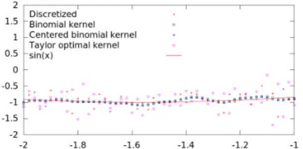
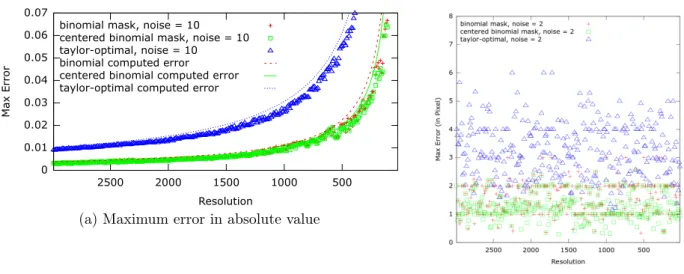
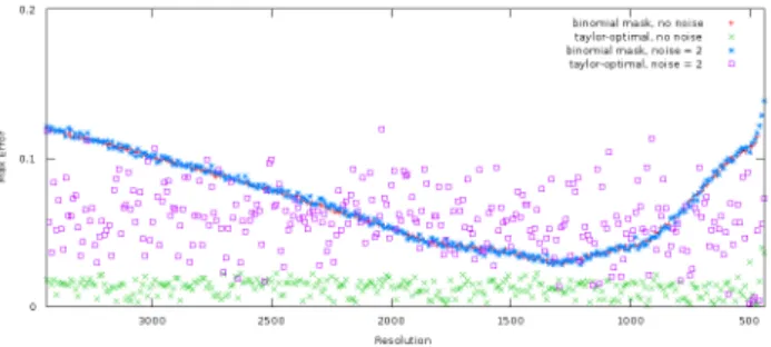
The last section is devoted to experiments, the main purpose of which are manly to illustrate the difference between masks, but also that only a few (typically a small constant such as 10 to 20 points) values are needed to obtain a good estimation. An appendix also proposes different criteria for choosing a mask, depending on the considered application.
Contents
1 Introduction 1
1.1 Aim of the work . . . 1
1.2 Outline . . . 3
2 Digitization, Quantization, Noise Models 5 3 Digital Derivatives for Functions 6 4 Basic Error Decomposition and Upper Bounds 8 4.1 Errors Related to Sampling and to Input Values . . . 8
4.2 Upper Bound for the Sampling Error . . . 8
4.3 Upper Bound for the Values Error . . . 9
5 Smoothing masks 10 5.1 Binomial Smoothing Masks . . . 10
5.2 Taylor-Optimal Smoothing Masks . . . 11
5.3 B−splines Smoothing Masks . . . 12
6 Skipping Masks: Cheap Multigrid Convergence 13 6.1 Uniform Multigrid Convergence with Uniform Noise or Bias . . . 13
6.2 Stochastic Multigrid Convergence with Stochastic Noise . . . 14
7 Examples of 1−derivative masks 14 7.1 Binomial 1−Derivative Mask . . . 14
7.2 Taylor-Optimal 1−Derivative Mask . . . 15
7.3 B−spline 1−Derivative Mask . . . 15
8 The cases of 2−Derivatives and Parametric Curves 16 8.1 Exemples of 2−derivative masks . . . 16
8.2 Parametrized Curves . . . 17 8.2.1 Binomial smoothing . . . 17 8.2.2 Discrete tangent . . . 17 8.2.3 Tangent Estimation . . . 17 8.2.4 Discrete curvature . . . 18 8.2.5 Curvature Estimation . . . 18
9 Piecewise Polynomial Functions and Convolutions 19
9.1 Continuous B−Splines Revisited . . . 19
9.1.1 Scaled B−Splines Curves Associated to a Sequence . . . 19
9.1.2 Derivative of the B−splines Curves with Skipped Control Points . . . 20
9.1.3 Relationship between scaled B−spline and convolutions . . . 21
9.2 Bézier Curves with Skipped Control Points . . . 21
9.2.1 Bézier Curves and Bernstein polynomials Basics . . . 21
9.2.2 Scaled Bézier Function Associated to a Sequence . . . 22
9.2.3 Derivative of the Scaled Bézier Function . . . 23
9.2.4 Binomial Convolutions and Scaled Piecewise Bézier . . . 24
10 Experiments 25 10.1 Smoothing . . . 25 10.2 Derivatives . . . 26 10.3 Curvature . . . 27 11 Conclusion 28 A Choosing a Mask 28 A.1 Criteria for Choosing a Mask . . . 28
A.2 Moments of The Main Considered Masks . . . 29
A.3 Smoothing Masks . . . 29
A.4 First Order Derivative Masks . . . 30
A.5 Second Order Derivatives . . . 31
2
Digitization, Quantization, Noise Models
Functions for which domain and range are sub-ring ofR, without any assumption on the nature of these sets, are called real functions. We call digital function a function fromZ to Z.
First we fix a model for the relationship between a continuous function and its digitization. Let f : R −→ R be a real function and let Γ : Z −→ Z be a digital function. Let h be the digitization step (i.e. the size of a pixel). We introduce a (possibly noisy) digitization of f .
Definition 2.1 The function Γ is a digitization of f with error ϵh with digitization step h on
the interval I if for any integer i such that ih∈ I we have:
hΓ(i) = f (ih) + ϵh(i) (1)
In order to apply this theory to signal analysis, we could distinguish two digitization steps for the domain and for the range, using the following definition: h2Γ(i) = f (ih1) + ϵh1,h2(i).
The results concerning the estimation errors bounds may be easily generalized to this frame-work. However generalized convergence results may hardly be efficient because of the many parameters involved.
We consider the following particular models for the errors ϵh on the values:
• Exact Values In this model, the values are known exactly: ϵh = 0
Note that, although this model has been the most widely used in approximation theory (e.g. [Flo05], [Flo08]), this value error model is not very realistic from an Information Sciences point of view.
• Uniform Noise (or Uniform Bias) on Values: In this model, the error ϵh on the values
is uniformly bounded by some constant which depends on the sampling step h. In our model, however, this bound can be asymptotically greater that h. Namely we assume here that
0≤ |ϵh(i)| ≤ Khα
where 0 < α≤ 1 and K is a positive constant. Note that this error can also have some bias, in the sense that the average noise value (or expected value) could be non-zero. This model has been considered by authors working on digital estimators based on thick digital lines.
• Quantization of Values: In this model, the errors ϵh on the values is uniformly bounded
by 12h. This is a particular case of uniform noise with α = 1, and corresponds to the
case when some basic quantization has been obtained by rounding-off the exactly known values of the function, for example for digital storage. This case is equivalent to Γ(i) = [
f (ih) h
]
. A variant is when quantization has been obtained by an integer part (floor case): 0 ≤ ϵh(i) < h , which is equivalent to Γ(i) = ⌊f (ih)h ⌋. This model is the most usual for
digital estimators based on digital lines.
• Stochastic Noise on Values: In this model, the errors ϵh(i) on the different values are
independent random variables with expected value 0 and standard deviation σ(h), con-verging to 0 along with h. For convergence results, we shall suppose σ(h)≤ Khα. This
model, and generally some estimators using measure theory, have been used recently ([CLMT15]), but, to the best of our knowledge, without any multigrid convergence re-sults.
3
Digital Derivatives for Functions
We introduce now a notion of digital derivatives.
Definition 3.1 (Digital Derivative) A digital ω-derivative mask is a sequence u = (u(i))i∈Z ∈ RZ of finite support such that
∑
i∈Z
iku(i) = 0 for 0≤ k < ω and ∑
i∈Z
iωu(i) = (−1)ωω!
Its associated digital ω-derivative operator is the function ∆u with domain RZ and co-domain
RZ defined by
∆u(v)(n) = (u ⋆ v)(n) =
∑
i∈Z
u(i)v(n− i).
Its convergence order is the greatest integer ρ such that for all integers k such that 1 + ω≤ k≤ ρ, we have ∑i∈Ziku(i) = 0.
Remark 3.1 Note that if there is no integer k such that 1 + ω≤ k and ∑i∈Ziku(i) = 0, then
the convergence order ρ is equal to ω.
Remark 3.2 In the case when the values u(i) are rational numbers and the sequence v has
integer values, then the values ∆u(v)(n) have rational values with denominator less than or
equal to the GCD of the denominators of the u(i).
Remark 3.3 Note that this definition of a derivative operator easily extends to some families
of sequences with infinite support, under some convergence hypothesis (e.g. rapidly decreasing masks like a sampling of the Gaussian). So, this definition can be extended to include scale-space notions ([Lin90]).
For the sake of clarity, we shall denote by ∆ωu the associated digital derivation operator of u when u is a digital ω-derivative mask. Intuitively, and as appears in the proofs below, the order ρ of an ω−derivative operator is the number of coefficients of the Taylor development of the function hω−11 ∆ωu(f )−f(ω)which vanish, minus one. As shown below, the convergence order
ρ will determine the speed of convergence of hω1−1∆ωu(f ) to f(ω), which is to distinguish from
the derivative order ω. Notice that the complexity of the computation is mainly dependent on the non zero coefficients of the mask, hence on the cardinality of its support (as long as it is computable). In [EMC11], this cardinal was an increasing function of h. One novelty of this work is considering masks with supports of constant cardinality, which is in practice so small as 10 or 12. Hence the computation needs no more than that number of products of integers. We shall use the following generalization of the classical finite difference operator with order 1 and skipping step l:
Definition 3.2 The following operator ∆+l is a digital 1−derivative operator:
∆+l (v)(n) = 1
l (v(n + l)− v(n)) the mask of which is defined by ∆+l (−l) = 1
l, and ∆ + l (0) =− 1 l and ∆ +
l (i) = 0 for others values
of i.
Similarly, we denote by ∆−l the following derivative operator:
∆−l (v)(n) = 1
l (v(n)− v(n − l))
As we could expect, the composition of two digital derivatives is also a digital derivative: Proposition 3.1 Let u = (u(i))i∈Z be an ω-derivative mask and v = (v(i))i∈Z be an ω′
-derivative mask. Then u ⋆ v is a ω + ω′-derivative mask. Proof. Let k ≤ ω + ω′. Then
∑ n∈Z nk(u ⋆ v)(n) = ∑n∈Z(i + (n− i))k∑ i∈Zu(i)v(n− i) = ∑n∈Z∑i∈Z∑kp=0(kp)ip(n− i)k−pu(i)v(n− i) = ∑kp=0(kp) (∑n∈Z∑i∈Zipu(i)(n− i)k−pv(n− i)) = ∑kp=0(kp) ∑j∈Z∑i∈Zipu(i)jk−pv(j) = ∑kp=0(kp) (∑j∈Zjk−pv(j)) (∑ i∈Zipu(i) )
This is zero except if k = ω + ω′ and in this case all the terms are zero except if p = ω and in this case the sum is (ω+ωω′ ′
)
(−1)ωω!(−1)ω′ω′! = (−1)ω+ω′(ω + ω′)!2
The following remark can be easily checked by induction on the degree of a polynom:
Remark 3.4 Our definition of a digital ω−derivative corresponds partially to the usual
deriva-tive when applied to polynomial sequences: let u be a digital ω-derivaderiva-tive mask with convergence order ρ and let v(i) be defined by ik for a given non negative integer k; then for k ≤ ρ, we have
(
∆ωu((ik)i∈Z)
)
(n) = k(k− 1)...(k − ω + 1)ik−ω.
4
Basic Error Decomposition and Upper Bounds
4.1
Errors Related to Sampling and to Input Values
In order to show that the digital ω-derivative of a digitization Γ of a real function f provides an estimate for the continuous derivative f(ω) of f , we would like to evaluate, at each sample
point, the difference between the digital derivative 1
hω−1(∆ ω
u⋆ Γ)(n) of the digitized signal and
the value of the usual ω−derivative f(ω)(nh) of f . This difference may easily be decomposed from Equation (1) and Definition 3.1 as the sum
1 hω−1(∆ ω u⋆ Γ)(n)− f (ω)(nh) = ES ω(f, h, Γ, u, n) + EVω(f, h, Γ, u, n) (2) where ESω(f, h, Γ, u, n) = ( 1 hω ∑ i∈Z u(i)f ((n− i)h) ) − f(ω)(nh) (3)
is called the sampling error, and
EVω(f, h, Γ, u, n) = 1 hω ∑ i∈Z u(i)ϵh(n− i) (4)
is called the values error. As their names imply, the sampling error is due to the fact that we only know about the values of f at some grid points, and the values error is due to the fact that we do not know the exact values of f at sample points.
The sampling error is a real values sequence. Under the uniform bias hypothesis, the values error is also a real valued sequence, but under the stochastic hypothesis, the values error is a sequence of random variable.
4.2
Upper Bound for the Sampling Error
In the following lemma, we show that the sampling error can be bounded independently from the error on input values, using the mask values, the norm of the k0-derivative of f , and a power
of the digitization step (namely hk0−ω), where k
0 is (at least in the case when f is sufficiently
regular) the convergence order of the mask u. The consequence is some convergence results in the case when exact values of the function at sample points are known.
Lemma 4.1 Let f be Ck on R, with k ≥ 1 + ω. Let u be a digital ω-derivative mask with
convergence order ρ. Let k0 = inf{k, 1 + ρ}. Let Γ be a digitization of f with step h on R.
Suppose that f(k0) is bounded on R. Then for all n,
|ESω(f, h, Γ, u, n)| ≤ hk0−ω ∥f(k0)∥ ∞ k0! ( ∑ i∈Z |ik0u(i)| ) Proof.
From Taylor formula, we first give an upper bound for the sampling error:
ES
ω(f, h, Γ, u, n) =
1
h
ω∑
i∈Zu(i)
(
i=k 0−1∑
j=0(
−ih)
jj!
f
(j)(nh) +
(
−ih)
k0k
0!f
(k0)(ζ(i))
)
− f
(ω)(nh)
where ζ(i) lies between nh and (n− i)h. From the definition of the order, we get:
ESω(f, h, Γ, u, n) = hk0−ω (−1)k0 k0! ( ∑ i∈Z ik0u(i)f(k0)(ζ(i)) ) |ESω(f, h, Γ, u, n)| ≤ hk0−ω ∥f(k0)∥ ∞ k0! ( ∑ i∈Z |ik0u(i)| ) 2
Example 4.1 From Definition 3.1, if f is C2 and a 1−derivative mask u has convergence
order 1, then the sampling error is O(h).
This is the case for the usual finite difference (∆(f )) (n) = f (n + 1)− f(n).
Example 4.2 Suppose that f is C3 and that a 1−derivative mask u has convergence order 2,
then the sampling error is O(h2).
This is the case for the usual symmetric finite difference (∆(f )) (n) = 12(f (n + 1)− f(n − 1)).
For a 2−derivative mask v with convergence order 2, the sampling error for the second derivative is O(h).
4.3
Upper Bound for the Values Error
The following lemma gives an upper bound for the error related to uniform noise or uniform bias on the values at sample points (see Section 2).
Lemma 4.2 Let f be a real function. Let u be a digital ω-derivative mask with convergence
order ρ. Let Γ be a digitization of f with step h on R and uniform bias ϵh such that ∥ϵh∥∞≤
Khα with 0 < α≤ 1. Then for all n,
|EVω(f, h, Γ, u, n)| ≤ K hω−α ( ∑ i∈Z |u(i)| ) Proof.
We straightforwardly give an upper bound for the values error:
|EVω(f, h, Γ, u, n)| ≤ ∥ϵh∥∞ hω ∑ i∈Z |u(i)| ≤ K hω−α ( ∑ i∈Z |u(i)| ) . 2
The following lemma gives an upper bound for the error related to statistic noise with expected values 0 on the values at sample points.
Lemma 4.3 Let f be derivable on R. Let u be a digital ω-derivative mask. Let Γ be a
digitization of f with step h on R and stochastic noise on values ϵh with expected value 0 and
standard deviation σ(h). Then for all n, the random variable 1 hω−1(∆
ω
u⋆ Γ)(n)− f
(ω)(nh) has
expected value ESω(f, h, Γ, u, n) and standard deviation σ(h)
hω
√∑
i∈Z(u(i))2. In other words,
and roughly speaking, the global error is in this case statistically close to the sampling error.
Proof. 1
hω−1(∆ ω
u⋆ Γ)(n)− f
(ω)
(nh) is equal to the sum of the constant value ESω(f, h, Γ, u, n)
and the random variable defined by EVω(f, h, Γ, u, n) = h1ω
∑
i∈Zuiϵh(n− i).
From linearity, its expected value is zero.
Since the random variables ϵh(n− i) are supposed to be independent and the support of u is
supposed to be finite, the square of the standard deviation of EVω(f, h, Γ, u, n) is equal to the
sum of the squares of the standard deviations of ui
hωϵh(n− i) which are
|ui|
hωσ(h). 2
Note that for a fixed mask, the values error (or its standard deviation) generally does not converge to zero when h converges to 0. We shall propose below a way to make it tend to zero by adapting the mask to the digitization step (see Theorem 6.1 and Theorem 6.2 below).
5
Smoothing masks
A smoothing mask is a 0−derivative mask. In this case, the values (∆0u⋆Γ)(n) may be considered
as partially de-noised values of f (nh). More precisely, under the uniform hypothesis, according to our upper bounds from Lemmas 4.2 and 4.1, the difference between h.(∆0
u⋆ Γ)(n) and f (nh)
cannot be considered not better (in order of magnitude) than the difference between h.Γ(n) and f (nh). Moreover, Lemma 4.3 with ω = 0 shows that, in the case of a stochastic noise on values, h.(∆0
u⋆ Γ)(n)− f(nh) is a random variable, the expected value of which converges to
0 along with h, and its standard deviation is less or equal than the one of h.Γ(n)− f(nh). Various choices for the smoothing masks may be considered. Here we focus on three families of masks.
5.1
Binomial Smoothing Masks
Definition 5.1 (Binomial Smoothing Masks) Let m be a positive integer and i be an
in-teger. The binomial smoothing mask with diameter (2m− 1) and cardinality 2m is the finite sequence of dyadic rational numbers B(0)2m−1 defined by B(0)2m−1(i) = 22m1−1
(2m−1
m−i
)
if −(m − 1) ≤ i≤ m, and by B(0)2m−1(i) = 0 in any other cases.
The binomial smoothing mask with diameter 2m and cardinality 2m+1 is the finite sequence of dyadic rational numbers B(0)2m defined by B(0)2m(i) = 22m1
(2m
m−i
)
if −m ≤ i ≤ m, and by
B(0)2m(i) = 0 in any other cases.
A unified definition may be B(0)r (i) = 21r
( r
⌈r
2⌉−i
)
if −⌊r2⌋ ≤ i ≤ ⌊r2⌋, and by B(0)r (i) = 0 in all
other cases.
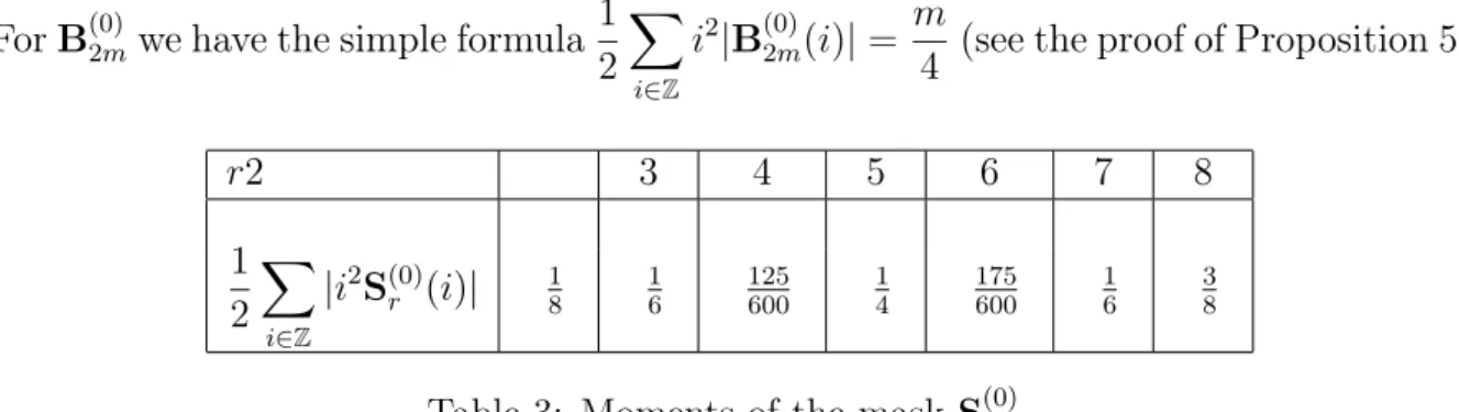
Proposition 5.1 The masks B(0)r for r ≥ 0, are discrete smoothing masks with convergence
Proof. We shall use the two following classical identities: i=n ∑ i=0 i ( n i ) = n2n−1 and i=n ∑ i=0 i2 ( n i ) = n(n + 1)2n−2. ∑ i∈Z B(0)2m−1(i) =∑ i∈Z
B(0)2m(i) = 1 are well known. ∑
i∈Z
iB(0)2m(i) = 0 come from parity. ∑ i∈Z iB(0)2m−1(i) = 1 22m−1 m ∑ i=−m+1 i ( 2m− 1 m− i ) = 1 22m−1 m ∑ j=0 (m− j) ( 2m− 1 j ) ∑ i∈Z iB(0)2m−1(i) = m− 1 2(2m− 1) = 1 2 ∑ i∈Z i2B(0)2m(i) = 1 22m m ∑ i=−m i2 ( 2m m− i ) = 1 22m m ∑ j=0 (m− j)2 ( 2m j ) ∑ i∈Z i2B(0)2m(i) = m2− 2m2+2m(2m + 1) 4 = m 2 2
5.2
Taylor-Optimal Smoothing Masks
The following so called Taylor-optimal smoothing mask is chosen having the best order as possible for a given diameter:
Definition 5.2 (Taylor-Optimal Smoothing Masks) Let m be a positive integer and i be
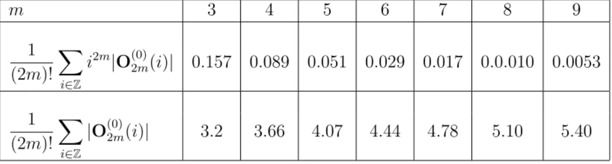
an integer. The Taylor-optimal smoothing mask with diameter 2m and cardinality 2m is the finite sequence of rational numbers O(0)2m defined by O(0)2m(i) = (−1)i+1 (
m |i|) (m+|i|m ) = (−1)i+1( 2m m+|i|) (2m m) if −m ≤ i ≤ m , and by O(0)
2m(i) = 0 in any other cases.
Proposition 5.2 The mask O(0)2m is a digital smoothing mask with convergence order 2m− 1. Proof. Let k ≥ 0. Let f be a polynomial and define the classical finite difference operator δ+
by δ+(f ) (x) = f (x + 1)− f (x). Iterating this operator leads to
δ2m+ (f ) (x) = 2m ∑ i=0 ( 2m i ) (−1)2m−if (x + i)
Applying this equality to the polynomials defined by (x− n)k for 0≤ k ≤ 2m − 1, we get
2m ∑ i=0 ( 2m i ) (−1)i(i + x− m)k = 0 Let now x = 0, then for all 0≤ k ≤ 2m − 1 we have
0 = 2m ∑ i=0 ( 2m i ) (−1)i(i− m)k = (−1)m j=m ∑ j=−m ( 2m m + j ) (−1)jjk
Hence for k = 1, we have ∑j=mj=−m,j̸=0(−1)j(2m
m+j
)
=−(2mm)and for 2≤ k ≤ 2m − 1, we have ∑j=m j=−m,j̸=0(−1) jjk(2m m+j ) = 0.
The same computation for the polynomial defined by (x− m)2m leads to
∑j=m j=−m,j̸=0(−1) jj2m(2m m+j ) = (−1)m ̸= 0. 2
5.3
B
−splines Smoothing Masks
Now, we define the B−spline Smoothing Kernels.
Definition 5.3 Let s ∈ Z. The Cox-De-Boor functions Ns,r (with knots ts = s), for r ∈ N,
are defined inductively as follows. Ns,0(t) =
{
1 if s≤ t < s + 1 0 otherwise.
For r≥ 1, we use the induction formula (called the Cox-de Boor formula): Ns,r(t) =
t− s
r Ns,r−1(t) +
s + r + 1− t
r Ns+1,r−1(t)
Lemma 5.1 We have Ni,r(t) = 0 for t ̸∈]i, i + r + 1[. Besides, for all t ∈ R and r ∈ N, we
have the following properties:
Partition of Unity Property: ∑
i∈Z Ni,r(t) = 1 Shift Property Ns,r(t + 1) = Ns−1,r(t) Symmetry Property Ns,r ( s + r+12 + t)= N0,r ( s + r+12 − t)
Proof. These properties are well known and follow immediately by induction from the Cox-de
Boor formula. 2
Definition 5.4 (B−spline Smoothing Masks) Let us consider a positive integer r ≥ 0.
We introduce a convolution mask (S(0)r (i))i∈Z with support included in {−⌊r+12 ⌋, . . . , ⌊r+12 ⌋},
based on the Cox-de Boor functions with degree r onR, with (bi-infinite) nodal vector τ = (i)i∈Z.
The mask values are defined by S(0)r (i) = N0,r(r+12 + i) = N−i,r(r+12 ) if −⌊r+12 ⌋ ≤ i ≤ ⌊r+12 ⌋ and
S(0)r (i) = 0 otherwise. This mask is called the uniform B−spline smoothing mask with degree
r.
Since N0,r(r+12 ) = 0, the cardinality of the mask S (0)
r is 2⌊r+12 ⌋. The mask is always
sym-metric.
Proposition 5.3 The mask S(0)r is a 0−derivative mask (i.e. a smoothing mask) with
conver-gence order 1.
Proof. The fact that S(0)r is a 0−derivative mask follows immediately from the partition of
Unity property in Lemma 5.1 and Definition 3.1. The convergence order (same definition) equal to 1 follows from:
∑ i∈Z i.S(0)r (i) =∑ i∈Z i.N0,r ( r + 1 2 + i )
The last sum is equal to zero from the symmetry property in Lemma 5.1. 2
The reader can find in Appendix A.3 some practical estimation for the constant involves in the asymptotic order sampling error for the three families of smoothing masks presented above.
6
Skipping Masks: Cheap Multigrid Convergence
The idea is adapting the mask to the step of digitization, in order to get 1
hω−α
(∑
i∈Z|u(i)|
) converging to zero along with h. For limiting the complexity of computation, we set the number of non zero coefficients of the mask fixed. This idea was independently used in [MB14] for length estimation. Other attempts have been considered in [GMES13].
Definition 6.1 (Skipping Masks) Let u be an ω-derivative mask with convergence order ρ,
and l ∈ N∗ be a skipping step. The corresponding ω-derivative l−skipping mask ul is defined
by ul(i) = l1ωu(il) if l divides i and 0 in any other cases. l is the length of the skips.
As ∑i∈Ziku
l(i) = lk−ω
∑
j∈Zjku(j), the mask ul is an ω-derivative mask with same
con-vergence order than u. But as ∑i∈Z|ul(i)| = l1ω
∑
j∈Z|u(j)|, it allows a convenient choice of l
depending on h in order to get a zero converging values error.
6.1
Uniform Multigrid Convergence with Uniform Noise or Bias
Theorem 6.1 Let u be an ω-derivative mask with order ρ and ulthe corresponding ω-derivative
l−skipping mask with skips of length l. Suppose that f : R −→ R is a Ck function and
f(k) is bounded, α ∈]0, 1], K ∈ R∗
+ and h ∈ R∗+. Suppose Γ : Z −→ Z is such that
|hΓ(i) − f(hi)| ≤ Khα for all i. Let k
0 = M in{k, 1 + ρ}. Then for k ≥ 1 + ω and
l(h) =⌊h−1+α/k0⌋, we have ( 1 hω−1∆ul(h)⋆ Γ ) (n)− f(ω)(nh) ∈ O(hα−ωα/k0),
and, for k = ω and l such that lim
h→0h.l(h) = 0 and limh→0 hα ((h.l(h))ω = 0, we have ( 1 hω−1∆ul(h)⋆ Γ ) (n)− f(ω)(nh) ∈ o(1).
Proof. First, we give an upper bound for the values error. From Lemma 4.2 and definitions,
we have EV (f, h, Γ, ul(h), n) ≤ l(h)ωKhω−α ∑ j∈Z|u(j)|. If l(h) = ⌊ h−1+α/k0⌋, it is easy to verify that 1 l(h)ωhω−α ≤ hα−ωα/k0 1− hω−ωα/k0 which is O(h α−ωα/k0).
We now turn to the sampling error:
• Let k ≥ 1 + ω. From Lemma 4.1 and definitions, the sampling error is less than
(l(h)h)k0−ω ∥f(k0)∥∞
k0!
∑
j∈Z|j
k0u(j)|. If l(h) =⌊h−1+α/k0⌋, it is easy to verify that|ES(f, h, Γ, u
l(h), n)| ≤ hα−ωα/k0∥f(k0)∥∞ k0! ∑ j∈Z|j k0u(j)|.
• Let f be Cω on R. From Taylor formula, ES(f, h, Γ, u
l(h), n) turn to be equal to
∑
j∈Zj
ωu(j)ϵ((n− jp(h))h), where ϵ is a function such that lim
x→0ϵ(x) = 0. 2
The multiplicative constants in the first part of Theorem 6.1 depends on various parameters. Some depend on informations about the data: a bound hmaxof the digitization step, or∥f(k0)∥∞
or K depending on the model of the noise. Some others depend on the mask: ∑i∈Z|iku i| is
named the k-moment of the mask. In the case when k≥ 1 + ω, the error is bounded by ( K 1− hα−ωα/k0 max ∑ i∈Z |uj| + ∥f(k0)∥ ∞ k0! ∑ i∈Z |jk0u j| ) hα−ωα/k0
For practical purposes, it could be useful to choose the mask in order to minimize this constant. In Appendix A.2, we provide formulas for some of our masks, and table of values for others.
6.2
Stochastic Multigrid Convergence with Stochastic Noise
Theorem 6.2 Let u be a ω-derivative mask with convergence order ρ and ul the corresponding
ω-derivative l−skipping mask. Suppose that f : R −→ R is a Ck function, with k ≥ 1 + ω,
and f(k) is bounded, α ∈]0, 1], K ∈ R∗+ and h ∈ R∗+. Let Γ be a digitization of f with step h and a stochastic noise ϵh with expected value 0 and standard deviation σ(h) ≤ Khα. Then for
k0 = M in{k, 1+ρ} and l(h) =
⌊
h1−α/k0⌋, the random variable
( 1
l(h)ω∆ul(h)⋆ Γ
)
(n)−f(ω)(nh)
has an expected value and a standard deviation which are O(hα−ωα/k0).
The proof is similar to that of Theorem 6.1.
7
Examples of 1
−derivative masks
It should be noted that all the masks defined in this section, which are digital 1−derivative (ω = 1) skipping masks, can be proven to have a multigrid convergence property either from Theorem 6.1 or from Theorem 6.2 (depending on the model of errors on values). We remind the reader that a more precise idea of the speed of convergence for the different masks can be found in Appendix A.2.
7.1
Binomial 1
−Derivative Mask
Definition 7.1 (Binomial skipping masks) Let m and l be positive integers and i be an
integer. The binomial 1−derivative l−skipping mask with diameter 2ml and cardinality 2m+1 for discrete first order derivation is the finite sequence of rational numbers B(1)l,2m−1 defined by
B(1)l,2m−1(i) = l22m1−1 (( 2m−1 m−1−il ) −(2m−1 m−il ))
if l divides i and−ml ≤ i ≤ ml, and by B(1)l,2m−1(i) = 0
in any other cases.
Remark 7.1 Note that B(1)l,2m−1 is the convolution product ∆+l ⋆B(0)l,2m−1. From Proposition 3.1, this is a general method for building a derivative mask from a smoothing mask.
Proposition 7.1 The masks B(1)l,2m−1 are discrete 1−derivative masks of convergence orders 2. Proof. We prove here the following equalities:∑
i∈ZB (1) l,2m−1(i) = 0 ∑ i∈ZiB(1)l,2m−1(i) =−1 ∑ i∈Zi 2B(1) l,2m−1(i) = 0 ∑ i∈Zi3B (1) l,2m−1(i) = 1−3m 2 l 2
Let us notice that for all k, we have: ∑ i∈Zi kB(1) l,2m−1 = lk−1 22m−1 ∑j=m j=−mj k((2m−1 m−1−j ) −(2m−1 m−j )) and ∑j=−1 j=−mj k((2m−1 m−1−j ) −(2m−1 m−j )) =∑j=mj=1 (−j)k((m2m−1+j−1)−(2mm+j−1)) ∑j=−1 j=−mj k((2m−1 m−1−j ) −(2m−1 m−j )) =∑j=mj=1 jk((2m−1 m−j ) −(2m−1 m−1−j )) Hence, for the even values of k, we have ∑i∈ZikBl,2m−1(i) = 0.
For the odd values of k, we have: ∑ i∈Zi kB(1) l,2m−1 = pk−1 22m−1 (∑j=m−1 j=−m j k(2m−1 m−1−j ) −∑j=m j=−m+1j k(2m−1 m−j )) ∑ i∈Zi kB(1) l,2m−1 = pk−1 22m−1 (∑j=m j=−m+1(j− 1) k(2m−1 m−j ) −∑j=m−1 j=−m j k(2m−1 m−j )) ∑ i∈ZikB (1) l,2m−1 = pk−1 22m−1 ∑j=m j=−m ( (j− 1)k− jk) (2m−1 m−j ) For k = 1, we get∑i∈ZiB(1)l,2m−1 =−1.
For k = 3, we use previous results: ∑ i∈ZikB (1) l,2m−1 = pk−1 22m−1 ∑j=m j=−m(−3j2+ 3j− 1) (2m−1 m−j ) ∑ i∈Zi kB(1) l,2m−1 = pk−1 22m−1(−3m.22m−2+ 3.22m−2− 22m−2) 2
Proposition 7.2 The masks B(1)l,2m are discrete 1−derivative masks of convergence orders 1.
The proof could be derived from Remark 7.1 and Proposition 3.1, or we could follow the first steps of the proof of Proposition 7.1.
7.2
Taylor-Optimal 1
−Derivative Mask
Definition 7.2 (Taylor-Optimal l−skipping masks) Let m and l be positive integers and
i be an integer. The Taylor-optimal 1−derivative l−skipping mask with diameter 2ml and cardinality 2m + 1 for discrete first order derivation is the finite sequence of rational numbers
O(1)l,m defined by O(1)l,m(i) = (−1) i l i (m | il |) (m+| il | m ) = (−1) i l i ( 2m m+| il |) (2m m)
if l divides i and −ml ≤ i ≤ ml, and by
O(1)l,m(i) = 0 in any other cases.
Let us note that the complexity of the computation depends mainly on the parameter m and a few on the parameter l.
Proposition 7.3 O(1)l,m are discrete 1−derivative mask with convergence order 2m .
The proof follows easily from Proposition 5.2.
7.3
B
−spline 1−Derivative Mask
Definition 7.3 (B−spline Derivative Kernel) Let us consider two integers r ≥ 0 and l > 0. We introduce a convolution mask S(1)l,r, with support in {−⌊lr2 + 1⌋, . . . , ⌊lr2 + 1⌋}, based on
the uniform Cox-de Boor functions with degree r− 1 on R. The mask values are defined by
S(1)l,r(i) = 1l (N0,r−1 (r 2 + i l ) − N0,r−1 (r 2 + i l − 1 ))
if l divides i and −⌊lr2 + 1⌋ ≤ i ≤ ⌊lr2 + 1⌋ and S(1)l,r(i) = 0 otherwise.
This mask is called the B−spline uniform l−skipping 1−derivative mask with degree r − 1.
Remark 7.2 Note that S(1)l,r = ∆−l ∗S(0)l,r−1, where S(0)l,r−1 denotes the l−skipping smoothing mask associated to the uniform B−spline smoothing mask S(0)r−1 with degree r− 1.
The proof could be derived from Remark 7.2 and Proposition 3.1, but we present a hand made proof.
Proof. The definition of a 1−derivative mask with convergence order 1 consists of two sum equalities. Hence the proof consists of two steps:
First Step. l∑i∈ZS(1)l,r(i) = ∑i∈lZN0,r−1 (r 2 + i l + 1 ) − N0,r−1 (r 2 + i l− 1 )
= 0. The last equality follows from change of index i↔ (i − l) in one of the sums.
Second Step. l∑i∈Zi.S(1)l,r(i) = ∑i∈lZi.[N0,r−1 (r 2 + i l ) − N0,r−1 (r 2 + i l − 1 )] = ∑i∈lZi.N0,r−1 (r−1 2 + i l ) −∑i∈lZ(i + l).N0,r−1 (r−1 2 + i l ) = −l∑i∈lZN0,r−1 (r−1 2 + i l ) =−l 2
The following methods for building derivative masks from a smoothing mask u of order ρ are worth noting:
1. Let v be the sequence defined by v(0) = ∑ 1
j∈Z,j̸=0u(j)
∑
j∈Z,j̸=0
1
ju(j) and v(i) =
−u(i) i∑j∈Z,j̸=0u(j)
for i̸= 0. Then, v is a 1−derivative mask with order 1 + ρ if and only if u(0) = 0. 2. From Proposition 3.1 and Definition 3.2, we can easily define and (ω + 1)−derivative
mask from any ω−derivative mask by covolution with ∆+l .. Evaluating the errors needs to evaluate ∑i∈Z|ikB(1)
l,2m−1(i)| and
∑
i∈Z|i kO(1)
l,m(i)| (see the
proof of Theorem 6.1). See Appendix A.4 for the most useful such estimations.
8
The cases of 2
−Derivatives and Parametric Curves
8.1
Exemples of 2
−derivative masks
Concerning second order derivatives, we can consider similar l−skipping masks. It is worth noting the following general method: Let u and v be two 1−derivative masks, then u ⋆ v is a 2−derivative mask (see Proposition 3.1).
Definition 8.1 Let m and l be positive integers and i an integer. The Taylor-optimal l−skipping
mask with diameter 2ml and cardinality 2m + 1 for discrete second order derivation is the finite sequence of rational numbers O(2)l,m defined by O(2)l,m(i) = −2li O(1)l,m(i) if l divides i and
−ml ≤ i ≤ ml and i ̸= 0 and O(2)
l,m(0) is such that ml
∑
i=−ml
O(2)l,m(i) = 0, and 0 for all other values
of i.
Lemma 8.1 O(2)l,m is a l−skipping 2−derivative mask with convergence order 1 + 2m.
The proof follows easily from Proposition 5.2.
Definition 8.2 Let m be a positive integers and i be an integer.
The binomial smoothing mask with diameter (2m+2)l and cardinality 2m+3 is the finite se-quence of rational numbers
( B(2)l,2m−1 ) defined by B(2)l,2m−1(i) = l222m1 −1 ((2m−1 m+1−i l ) − 2(2m−1 m−i l ) +(m2m−1−−1i l ))
if −(m + 1)l ≤ i ≤ (m + 1)l and l divides i, and by B(2)l,2m−1(i)) = 0 in any other cases. See Appendix A.5 for estimations of constants in the convergence order.
8.2
Parametrized Curves
Let k≥ 1. We assume that a planar closed Ck-parametrized curve C (i.e. the parametrization
is periodic) is given together with a family of parametrized digital curves (Σh) with Σhcontained
in a tube with radius H(h) around C. A parametrization of C is denoted by g = (g1, g2) :
R 7→ R2, where g
1 and g2 are C1 and periodic with a common period. The parametrization of
Σh is denoted by Γh = (Γ1, Γ2) :Z 7→ Z2.
8.2.1 Binomial smoothing
Let P = (P0, . . . , Pn) be a (n + 1)−tuple of control points. Let us denote a Bézier curve
BP(t) = ∑n i=0 (n i ) ti(1− t)n−i.P
i, where t∈ [0, 1] (See the Section 9.2). Thus we have
B(Γ(i0−m+ζ),...Γ(i0+m))( 1 2) = (( ∆0 B(0)2m−ζ(Γ1) ) (i0), ( ∆0 B(0)2m−ζ(Γ2) ) (i0) ) where ζ = 0 or 1. 8.2.2 Discrete tangent
Here we estimate the tangent at a point of C by a digital tangent at a not too far point of Σh.
To this purpose, we define the digital derivative in a natural way with the digital derivative of the coordinates. Note that this definition needs no hypothesis concerning the parametrized curve. Moreover, we could theoretically use different masks for the two coordinates. For sake of simplicity, we shall use the same for both.
Definition 8.3 Let u be a 1−derivative mask. Let Γ = (Γ1, Γ2) : Z 7→ Z × Z be a digital
parametrization of a digital curve Σ.
The digital derivative of Γ at point Γ(n) is
(( ∆1u(Γ1) ) (n),(∆1u(Γ2) ) (n)) It is denoted by (∆1
u(Γ)) (n). When this vector is nonzero, the corresponding discrete tangent
at Γ(n) is the real line going through Γ(n) directed by (∆1
u(Γ)) (n).
Let us notice that the asymmetric l−skipping binomial case corresponds to the derivative of the Bézier curve with control points (Γ(i0− (m − 1)l), ..., Γ(i0+ ml)) computed at the
medial-point of parameter 12.
8.2.3 Tangent Estimation
Theorem 8.1 Let u be a smoothing mask with convergence order ρ. Let g = (g1, g2) be a Ck
parametrization of a closed curve Σ. Let k0 = inf{k, 1 + ρ}, α ∈]0, 1], K ∈ R∗+ and h ∈ R∗+
with h≤ 1
2. Let Γh = (Γh,1, Γh,2) :Z 7→ Z × Z be a digital parametrization of Σ. Suppose that
for all i we have ∥g(ih) − h.Γh(i)∥∞ ≤ Khα. Suppose that g
(k0) c is bounded for c = 1, 2. Then ∥∆1 u(Γh)(n)− g′(nh)∥∞ is less than hk0−1 M ax { ∥g(k0) 1 ∥∞,∥g (k0) 2 ∥∞ } k0! ( ∑ i∈Z |ik0u(i)| ) + K h1−α ( ∑ i∈Z |u(i)| )
The proof follows directly from Lemma 4.2 and Lemma 4.1.
Theorem 8.2 Let u be a 1−derivative mask with convergence order ρ and ul the
corre-sponding 1−derivative l−skipping mask. Under the hypothesis of Theorem 8.1, for k ≥ 1 and l(h) = ⌊h−1+α/k0⌋we have ∆1
ul(h)(Γh)(n)− g
′(nh)
∞ ∈ O(h
α−α/k0), and for k = 1 and
l(h) =⌊h−1+α/2⌋, we have ∆1
ul(h)(Γh)(n)− g
′(nh)
∞ ∈ o(1)
The proof is straightforward.
The hypothesis of Theorem 8.1 is stronger than the digitization being simply contained in a tube, because not only the discrete curve must be close to the continuous curve, but the parametrization of the digitization must be close to the parametrization of the continuous curve. This was the reason for introducing Pixel-Length parametrizations in [EMC11].
8.2.4 Discrete curvature
We estimate the curvature at a point of C by a digital curvature at a not too far point of Σh. The definition of the digital curvature coincides with the classical formula for continuous
curves.
Definition 8.4 Let u and v be respectively a 1−derivative mask and 2−derivative mask. Let Σ be a digital parametrized curve of parametrization Γ = (Γ1, Γ2). The corresponding discrete
curvature at Γ(n) is (∆2 v(Γ1)) (n) (∆1u(Γ2)) (n)− (∆1u(Γ1)) (n) (∆2v(Γ2)) (n) ( ((∆1 u(Γ1)) (n)) 2 + ((∆1 u(Γ2)) (n)) 2)3/2
when the vector ∆1u(Γ)(n) is non-zero. It will be denoted by Cu,v(Γ)(n).
Notice that this definition needs no more hypothesis concerning the parametrized curve.
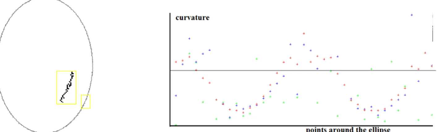
8.2.5 Curvature Estimation
We shall denote γg(t) the curvature of a curve parametrized by g at the point of parameter
t. The following convergence theorem required some additional hypothesis concerning the
regularity of the considered point.
Theorem 8.3 Let u be a 1−derivative mask with convergence order ρ(u) and ul the
corre-sponding 1−derivative l−skipping mask.
Let v be a 2−derivative mask with convergence order ρ(v) and vlthe corresponding 2−derivative
l−skipping mask.
Let g = (g1, g2) be a Ck parametrization of a simple closed curve, with k ≥ 2.
Let Γ = (Γ1, Γ2) :Z 7→ Z × Z be a digital parametrization of a digital curve Σ.
Let k0 = inf{k, 1+ρ(u), 1+ρ(v)}, α ∈]0, 1], K ∈ R∗+ and h∈ R∗+ and h ≤ 12. Suppose that for
all i we have ∥g(nh) − h.Γ(n)∥∞ ≤ Khα. Suppose that g(k0)
c is bounded for c = 1, 2. Suppose
that for t∈ [t1, t2], the vector g′(t)̸= 0.
Then, there is some h0 > 0 and two functions n1, n2 : (0; +∞) 7→ Z such that for l(h) =
⌊ h−1+α/k0⌋, for h≥ h 0 and n∈ [n1(h), n2(h)]∩ Z, we have Cul(h),vl(h)(Γ)(n)− γg(nh) ∈ O(hα−2α/k0)
Proof. Let us introduce the function defined onR2− {(0, 0)} × R2 by F (X, Y, Z, T ) = ZY − XT (X2+ Y2)32 Hence Cul(h),vl(h)(Γ)(n) = F (∆ 1 ul(h)(Γ)(n), ∆ 2 vl(h)(Γ)(n)) and γg(nh) = F (g ′(nh), g”(nh)).
The differential of F is easily seen to be bounded on any compact K in R2− {(0, 0)} × R2. Let MK be one of its upper bounds on K. Then for a and b in K, we have∥F (a) − F (b)∥∞≤
MK∥a − b∥∞.
We claim that, under the hypothesis of the theorem, we know that there is a compact K1
inR2− {(0, 0)} such that for t ∈ [t
1, t2]⊂ R, the derivative g′(t) lies in K1. Indeed K1 ={x ∈
R2; α ≤ ∥x∥ ≤ β}, where α = Inf{∥g′(t)∥; t ∈ [t
1; t2]} and β = Max{∥g′(t)∥; t ∈ [t1; t2]} is
convenient.
Then from Theorem 8.2, we can find a compact K2 in R2− {(0, 0)} and a fixed h1 such
that for h≥ h1 and n∈ [⌈th1⌉, ⌊th1⌋] ∩ Z the derivatives g′(nh) and (∆1ul(h)(Γ)(n) ly in K2.
Moreover, under previous conditions, the second order derivatives g”(nh) and (∆2
vl(h)(Γ)(n)
lie in a compact K3 of R2.
From Theorem 6.1, there is a constant χ and a fixed h2 such h≥ h2, we have
(∆1 ul(h)(Γ)(n), ∆ 2 vl(h)(Γ)(n))− (g ′(nh), g”(nh)) ∞ ≤ χ.h α−2α/k0
Hence for h≥ max{h1, h2} and n ∈ [n1(h), n2(h)]∩ Z, we have
Cul(h),vl(h)(Γ)(n)− γg(nh) ∞ ≤ χ.MK2×K3.h α−2α/k0 2
9
Piecewise Polynomial Functions and Convolutions
9.1
Continuous B
−Splines Revisited
9.1.1 Scaled B−Splines Curves Associated to a Sequence
Let E be an R−module and let (Γ(s))s∈Z be a sequence with values in E. Let r ∈ N. The
uniform B−spline function with degree r and control points (Γ(s))s∈Z is defined by:
( S(0) 1,r(Γ) ) (t) =∑ s∈Z Γ(s)Ns,r(t)
where the Ns,r function is the Cox De-Boor function (see Definition 5.3).
Definition 9.1 Let l ∈ N∗+ and r ∈ N. First, for s ∈ Z we define the l−scaled B−spline
function Ns,r,l by:
Ns,r,l(t) = Ns,r(
t
Definition 9.2 The uniform l−scaled B−spline function with degree r associated to Γ is defined by: ( S(0) l,r(Γ) ) (t) =∑ s∈Z Γ(ls)Ns,r,l(t)
Note that this last function can be interpreted a regular uniform B−spline functions control points (Γ(ls))s∈Z with difference between successive nodal points equal to l.
Definition 9.3 Let Φ :Z −→ E be a sequence, or Φ : R −→ E be a function.
We denote by τ (Φ) the right shift of Φ which to s associates (τ (Φ)) (s) = Φ(s + 1).
The following property follows immediately from the shift property in Lemma 5.1.
Property 9.1 ( S(0) l,r(τ l (Γ)) ) (t) = ( τl(Sl,r(0)(Γ)) ) (t)
9.1.2 Derivative of the B−splines Curves with Skipped Control Points
As far as the Cox de-Boor functions are concerned, we have the classical expression for the derivative:
Ns,r′ (t) = (Ns,r−1− Ns+1,r−1)
From the definition of Ns,r,l(t) we get
Ns,r,l′ (t) = 1 lN ′ s,r( t l) = 1 l (Ns,r−1,l(t)− Ns+1,r−1,l(t)) (6)
Proposition 9.1 For r∈ N∗ we have: d dt ( S(0) l,r(Γ) ) (t) = 1 l ( S(0) l,r−1(Γ)− S (0) l,r−1(τ−l(Γ)) ) Proof. d dt ( S(0) l,r(Γ) ) (t) = ∑s∈ZΓ(ls)Ns,r,l′ (t) = ∑s∈ZΓ(ls)1l (Ns,r−1,l(t)− Ns+1,r−1,l(t)) = ∑s∈ZΓ(ls)1l (Ns,r−1,l(t))−∑s∈ZΓ(l(s− 1))1l (Ns,r−1,l(t)) = 1 l ∑ s∈Z ( Γ(ls)− τ−lΓ(ls))(Ns,r−1,l(t)) 2
Definition 9.4 Let Φ :Z −→ E be a sequence, or Φ : R −→ E be a function. We denote (
∆−l (Φ))(s) = 1
l(Φ(s)− Φ(s − l)).
Notation 9.1 For ω ≤ r − 1, we denote by Sl,r(ω)(Γ) the function defined on R by: ( S(ω) l,r (Γ) ) (t) = d ω dtω ( S(0) l,r (Γ) ) (t)
With these notations, Proposition 9.1 can be reformulated as S(1) l,r(Γ) = ( ∆−l ( S(0) l,r−1(Γ) )) Hence by induction, we get:
Proposition 9.2 For ω ≤ r − 1, we have
S(ω) l,r (Γ) = (( ∆−l )ω ( S(0) l,r−ω(Γ) ))
9.1.3 Relationship between scaled B−spline and convolutions Proposition 9.3 For n∈ Z, we have
( S(0) l,r(Γ) ) ( l ( n + r + 1 2 )) = ( S(0)l,r ∗ Γ ) (n) Proof. ( S(0) l,r (Γ) ) ( l(n + r+12 )) = ∑s∈ZΓ(ls)Ns,r,l(l(n + r+12 )) = ∑s∈ZΓ(ls)Ns,r(n + r+12 ) = ∑s∈ZΓ(ls)N0,r(r+12 + n− s) = ∑s∈ZΓ(ls)S(0)l,r(n− s) = ( S(0)l,r ∗ Γ ) (n) 2
Notation 9.2 For ω ∈ {0, . . . , r − 1}, we denote S(ω)l,r =(∆−l )ω
( S(0)l,r−ω
)
Note that, from Proposition 3.1, the mask S(ω)l,r is an ω−derivative mask. Theorem 9.1 For n∈ Z and ω ∈ {0, . . . , r − 1}, we have
( S(ω) l,r (Γ) ) ( l ( n + r + 1 2 )) = ( S(ω)l,r ∗ Γ ) (n)
9.2
Bézier Curves with Skipped Control Points
9.2.1 Bézier Curves and Bernstein polynomials Basics
Definition 9.5 Let r∈ N∗. For i∈ 0, . . . , r, we consider the R−valued polynomial with degree r defined by Bi,r(t) = ( r i ) ti(1− t)r−i
In the sequel, unless otherwise specified, we shall say Bernstein polynomials or Bernstein functions as a shorthand for Bernstein polynomials. The Bernstein polynomials with degree r constitute a basis of the vector space of polynomials with degree less than or equal to r.
From the Pascal formula for binomial coefficients, we derive a similar formula about Bern-stein polynomials:
Bi,r(t) = (1− t)Bi,r−1(t) + tBi−1,r−1(t) (7)
Definition 9.6 Let E be an R−module and let P = (P0, . . . , Pr−1) be a sequence of point in
E. Let BP : 1−→ E be the Bézier Curve with control points P. Then we have:
BP(t) = r−1
∑
i=0
PiBi,r−1(t)
We can compute the derivative of a Bézier Curve as follows. Let BP : [0, 1]−→ E be the
Bézier Curve with control points P0, . . . , Pr−1. Then we have:
BP′ (t) = (r− 1)
r−2
∑
i=0
(Pi+1− Pi)Bi,r−2(t)
which is the Bézier curve with control points P1′, . . . , Pn′−1, where Pi′ = (r− 1)(Pi+1− Pi).
9.2.2 Scaled Bézier Function Associated to a Sequence
Definition 9.7 Let l∈ N∗+. We introduce the s−shifted l−scaled Bernstein polynomials by: Bi,s,r,l(t) = { Bi,r (t l − s ) if tl ∈ [s, s + 1[ 0 otherwise.
In other words, the value Bi,s,r,l(t) can be non-zero only for s = ⌊tl⌋. In the remainder of
this section, E denotes anR−module and (Γ(s))s∈Z is a sequence with values in E.
Definition 9.8 Let l∈ N∗+. The l−scaled (piecewise) Bézier curve with degree r−1 associated
to Γ is defined over R by: ( B(0) l,r(Γ) ) (t) =∑ s∈Z r ∑ i=0 Γ (l(s + i− r)) Bi,s,r,l(t)
Note that in the previous definition, due to the definition of Bi,s,r,l, for a given value of i, only
one value of s (namely s = ⌊tl⌋ + r − i) contributes to the double sum (
B(0)
l,r(Γ)
)
(t), so that, in fact, at most r + 1 terms are non-zero.
Proposition 9.4 (De Casteljau Property) ( B(0) l,r(Γ) ) (t) = ( ⌊t l⌋ + 1 − t l) ) ( B(0) l,r−1(τ−l(Γ)) ) (t) + ( t l − ⌊ t l⌋ ) ( B(0) l,r−1(Γ) ) (t)