2PAC: Two Point Attractors for Center of Mass Trajectories in Multi Contact Scenarios

HAL Id: hal-01609055

https://hal.archives-ouvertes.fr/hal-01609055v2

Submitted on 17 Jul 2018

HAL is a multi-disciplinary open access

archive for the deposit and dissemination of

sci-entific research documents, whether they are

pub-lished or not. The documents may come from

teaching and research institutions in France or

abroad, or from public or private research centers.

L’archive ouverte pluridisciplinaire HAL, est

destinée au dépôt et à la diffusion de documents

scientifiques de niveau recherche, publiés ou non,

émanant des établissements d’enseignement et de

recherche français ou étrangers, des laboratoires

publics ou privés.

Trajectories in Multi Contact Scenarios

Steve Tonneau, Pierre Fernbach, Andrea del Prete, Julien Pettré, Nicolas

Mansard

To cite this version:

Steve Tonneau, Pierre Fernbach, Andrea del Prete, Julien Pettré, Nicolas Mansard. 2PAC: Two Point

Attractors for Center of Mass Trajectories in Multi Contact Scenarios. ACM Transactions on Graphics,

Association for Computing Machinery, 2018, 37 (5), pp.176. �10.1145/3213773�. �hal-01609055v2�

Trajectories in Multi Contact Scenarios

STEVE TONNEAU,

PIERRE FERNBACH,

ANDREA DEL PRETE,

JULIEN PETTRÉ,

NICOLAS MANSARD,

Synthesizing motions for legged characters in arbitrary environments is a long-standing problem that has recently received a lot of attention from the computer graphics community. We tackle this problem with a procedural approach that is generic, fully automatic and independent from motion capture data. The main contribution of this paper is a point-mass-model-based method to synthesize Center Of Mass trajectories. These trajectories are then used to generate the whole-body motion of the character.

The use of a point mass model results in physically inconsistent motions and joint limit violations when mapped back to a full- body motion. We mitigate these issues through the use of a novel formulation of the kine-matic constraints which allows us to generate a quasi-static Center Of Mass trajectory, in a way that is both user-friendly and computationally efficient. We also show that the quasi-static constraint can be relaxed to generate motions usable for computer animation, at the cost of a moderate violation of the dynamic constraints.

Our method was integrated in our open-source contact planner and tested with different scenarios - some never addressed before- featuring legged characters performing non-gaited motions in cluttered environments. The computational efficiency of our trajectory generation algorithm (under one ms to compute one second of trajectory) enables us to synthesize motions in a few seconds, one order of magnitude faster than state-of-the-art methods. Although our method is empirically able to synthesize collision-free motions, the formal handling of environmental constraints is not part of the proposed method, and left for future work.

CCS Concepts: • Computing methodologies → Procedural animation; Physical simulation;

Additional Key Words and Phrases: Character animation, multi contact locomotion, motion planning, center of mass

ACM Reference format:

Steve Tonneau, Pierre Fernbach, Andrea Del Prete, Julien Pettré, and Nicolas Mansard. 2018. 2PAC: Two Point Attractors for Center of Mass Trajectories in Multi Contact Scenarios. ACM Trans. Graph. 1, 1, Article 1 (July 2018), 14 pages.

https://doi.org/0000001.0000001_2

1 INTRODUCTION

The automatic synthesis of complex motions for legged characters is an open problem, actively researched by both the computer graphics and the robotics communities. One challenge is to provide charac-ters with enough autonomy of motion so as to facilitate character animation tasks, or to animate non-player characters in games. Ide-ally, a method to synthesize believable motions would only require © 2018 Association for Computing Machinery.

This is the author’s version of the work. It is posted here for your personal use. Not for redistribution. The definitive Version of Record was published in ACM Transactions on Graphics, https://doi.org/0000001.0000001_2.

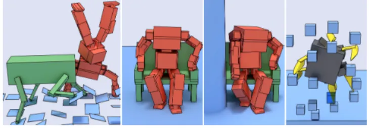
Fig. 1. Multi contact motions synthesized by our method.

simple high level inputs (e.g., initial and final positions), and not tedious manual editing from an animator. It would also generalize well to large sets of legged characters (with any number of legs), and would not require the gathering of large motion capture datasets for each character. It would not be restricted to flat ground or annotated environments. Finally, it would be computationally efficient, close to real time. This would allow for online motion generation appli-cations, and not let animators wait for too long before obtaining a result. In this paper, we consider the problem of computing a physi-cally plausible motion between two positions for a legged character in an arbitrary environment. We demonstrate significant progress with respect to all the objectives listed above: generalization over various characters, physical accuracy and plausibility, environment variety and complexity, computational performance.

This problem has received significant attention over the past decade. As a result, the synthesis of walking or running motions in open environments (flat ground, few obstacles) is now commonly and efficiently addressed by existing methods [Kajita et al. 2003; Yin et al. 2007]. In this context, where the contact phases are cyclic, the kinematic constraints of the avatar can be easily expressed [Perrin et al. 2012]. Furthermore the dynamics of the avatar can be accu-rately approximated by assuming that the ground is always flat. Multi contact locomotion is the general case that we consider, where all these simplifying assumptions no longer hold. Examples of multi contact motions include climbing, walking on highly uneven terrain or climbing stairs using a handrail. The issue of finding when, where and with which effector to create a contact leads to a high dimen-sional combinatorial problem. Additionally, the dynamics of the system is more complex, and the kinematic constraints are harder to express. Finally, motions occur in the proximity of obstacles which makes the collision avoidance non trivial. As a result, motion synthe-sis is hard to generalize because small changes in the environment affect significantly the solution space.

A common approach is to reduce the dimension of the problem by considering a point mass model (3 degrees of freedom) rather than the complete avatar (60 degrees of freedom), and then focus on planning a trajectory for the center of mass (COM), with sig-nificant success. However, this approximation often leads to joint limit violations once the whole-body motion is computed. More-over, the angular momentum generated by the character bodies is unknown when computing the COM trajectory, so there is no guarantee that the resulting motion will be dynamically consistent. Furthermore, finding a trajectory is usually formulated as a non-convex optimization problem, computationally expensive, with no guarantee of convergence.

In this paper we propose a different approach to provide gua-rantees of kinematic and dynamic feasibility. Rather than relying on a simplified model, we first consider a conservative but exact formulation of the dynamics, later relaxed while preserving the kinematic constraints of the motion. Our approach is agnostic to the character morphology, allowing us to consider a large range of complex environments.

Our method is described by two steps. In a first step we restrict ourselves to quasi-static locomotion, where the robot moves at low velocity. In this context the point mass model dynamics is accurate because the angular momentum is negligible. The linear momentum is not, because it is required to verify that it is possible to generate the forces compensating the gravity interaction. By considering a new approximate formulation of the kinematic constraints, we show that finding a trajectory connecting two contact phases boils down to finding a single point that uniquely defines such a solution, and which can be computed efficiently. In a second step we show that we can relax the quasi-static constraint to generate smoother trajectories while preserving the kinematic constraints, in a flexible way that can be parametrized by the user. Thanks to this property, our method is robust to failures and always proposes a solution, assuming one exists.

Our main contribution is thus a fully automatic and procedural method to compute a kinematically feasible, quasi-static COM tra-jectory in multi contact situations, for arbitrary creatures, envi-ronments and scenarios. This is achieved thanks to two technical contributions:

(1) a new formulation of the kinematic constraints for the point mass model;

(2) a one-step algorithm to compute a feasible trajectory, the fastest to our knowledge.

Additionally, we demonstrate that our method can be integrated with an open-source contact planner to generate whole-body mo-tions in a large variety of scenarios.

1.1 Situation of the contribution with respect to the authors’ previous work

In this work, to present our results we use a previously published contact planner [Tonneau et al. 2015, 2018]. This contact planner generates a sequence of discrete key postures in contact. The method proposed in this paper is concerned with the interpolation of the sequence into a continuous motion. The combinatorial aspect in the choice of contacts is handled by the planner, and thus not discussed

in this paper. The planner is considered as a black box that generates the contact sequence, and the paper focuses on the generation of a trajectory for the Center Of Mass of the robot. Section 7 presents the global architecture of the framework (including the planner), and includes the planning timings in our performance reports. However the reader is referred to [Tonneau et al. 2018] for details on the planner, which is not mandatory to implement the method. Typically, the contact sequence could be provided by a user or another contact planning technique. In all other sections, the contributions described are thus novel.

2 STATE OF THE ART

The synthesis of multi contact locomotion is a subject of rising inter-est for both the robotics and computer graphics communities, which follows many years of research on gaited locomotion. It remains largely open due to the difficulty of handling arbitrary environ-mental constraints in a high-dimensional space. Both procedural and data-driven approaches currently converge towards simplified models for handling the complex dynamics of legged characters. We believe that improving these models is the key to synthesizing more realistic motions.

To account for the variety of approaches and the complexity of the topic, this state of the art considers the problem in its entirety, before focusing on the particular topic of our concern, the fast generation of dynamically consistent centroidal trajectories.

2.1 Procedural approaches to multi contact locomotion

After years of research, efficient simplifying models have been pro-posed to synthesize walking or running motions on the fly, such as the linear inverted pendulum model [Kajita et al. 2003] which led to the introduction of the capture point [Pratt et al. 2006]. Some of them are able to handle terrain deformations [Englsberger et al. 2015]. A large part of the state of the art has investigated the generation of more varied gaited motions. To achieve such results, they progres-sively introduced machine learning methods within physics-based controllers, to extend their range of applications while obtaining more robust controllers [Coros et al. 2009; de Lasa et al. 2010; Peng et al. 2016, 2017]. Our approach differs because we do not assume a gait, or a determined behavior that must be followed at best, but rather try to achieve motion generation in cases where the “correct” behavior to follow is unknown (for instance in constrained envi-ronments). As a consequence, our results are more generic but less impressive than these methods.

Whole-body dynamic solvers have also been proposed to syn-thesize non-gaited, highly dynamic motions [Al Borno et al. 2012]. Similarly, reactive multi contact controllers follow local control policies using a small planning horizon that results in myopic be-haviors [Hämäläinen et al. 2015; Jain et al. 2009]. Recent work try to generalize these controllers by using them within new sampling based algorithms [Al Borno et al. 2017]. Recently [Naderi et al. 2017] also proposed to combine these approaches with a global planner, thus reintroducing a combinatorial issue, which may be difficult to scale beyond climbing scenarios with discrete sets of grasping locations. These works, in the continuity of seminal ones from [Bretl et al. 2004] and [Escande et al. 2013], illustrate the main issue of

Method Kinematic model contact model Dynamic model computation

times (≈ 10 contacts) avatars application [Tonneau et al. 2015] (planning) +Ours(trajectory) Approximated 6D Quasi-static point mass seconds (planning)

ms (COM trajectory) Any

Any, including highly constrained

partial collision handling

[Carpentier et al. 2016]

[Herzog et al. 2015] Approximated 6D

Dynamic

point mass

seconds

(COM trajectory) Any

Any

no collision handling

[Mordatch et al. 2012] No joint limits 6D Quasi-static

point mass Minutes (planning + COM trajectory) Any Any no collision handling

[Kang and Lee 2017] Approximated

(Learned)

effector slipping

Quasi-static point mass, only valid

on flat terrain Several seconds to Minutes (planning + Whole-body motion) Humanoid Climbing partial collision handling

[Naderi et al. 2017] Exact 3D Exact

Minutes (planning + Whole-body motion) Any Climbing, discretized contact locations

full collision handling Table 1. Comparison of the main methods in the literature for the complete issue of both planning and generating a multi contact whole-body motion.

multi-contact locomotion, which consists in finding the acceptable trade-off between a complete approach subject to combinatorial explosion on one hand, and an efficient method subject to local min-ima on the other hand. Our choice is the decomposition between the contact planning and the trajectory generation problems, with a contact planning approach that remains linear with respect to the complexity of the environment. While the cost for this efficiency is the introduction of approximations which can lead to failures, its empirical interest is demonstrated and discusssed in [Tonneau et al. 2018].

In this paper, we focus on an integration of the presented method within our contact planner, but our contribution is compatible with other approaches, such as [Naderi et al. 2017]. In such a case, the global planner would call our method rather than the proposed local policy, to obtain faster yet approximated results. In any case, the inputs of the method remain the same: a discretized sequence of contacts, used to solve a local trajectory optimization problem.

[Mordatch et al. 2012] and [Deits and Tedrake 2014] also compute simultaneously the trajectory of the avatar and the contact locations, through the formulation of a nonconvex optimization problem. In-terestingly, they obtained better computation times thanks to the use of a simplifying point mass model to reduce the dimension of the problem. Some approaches that decouple contact planning and trajectory optimization also rely on simplified models, during both the contact planning sequence [Grey et al. 2017; Tonneau et al. 2015] and the trajectory generation [Carpentier et al. 2016; Herzog et al. 2015]. However, the trajectory generation methods use non-linear resolution methods that are not guaranteed to converge. More im-portantly, although they demonstrate interactive computation times (a few hundred milliseconds to compute), they are not fast enough

to consider real time applications. Our objective is to go below the millisecond of computation.

2.2 Data driven approaches and the arrival of learning methods

In parallel to procedural approaches, data driven methods are able to synthesize complex movements by connecting motion clips within a graph structure [Kovar et al. 2002; Lau and Kuffner 2006], before performing motion deformation to adapt the motion to a new en-vironment [Choi et al. 2003; Ho et al. 2010; Witkin and Popovic 1995], even for large deformations [Han et al. 2016; Tonneau et al. 2016]. However, these methods only apply to motions that present the same contact pattern as those used in the provided data, and thus similar environments. As for physics based approaches [Peng et al. 2017], the introduction of deep learning techniques holds the promise of a breakthrough towards the generality of data driven approaches [Holden et al. 2017]. The first learning paper to directly address multi contact locomotion was by [Kang and Lee 2017], but remains limited to a single type of morphology (a human).

2.3 Simplified models for efficient motion generation

The recent successes in multi contact locomotion share the common idea of simplifying the dynamics of the character, which results in a faster solution of the problem. [Kang and Lee 2017] check whether the COM of the robot lies above the convex hull of the contact points to determine whether the robot is in equilibrium. However, this condition is neither necessary nor sufficient in the multi contact case, and is only valid to verify static equilibrium (i.e. when the acceleration of the COM is null) for coplanar contact points [Del Prete et al. 2016; Guo et al. 2015]. But, even with an

accurate formulation of the dynamics [Qiu et al. 2011], using the point mass model results in a loss of information on the angular momentum generated by the limbs, which can make the character lose equilibrium.

The other important piece of information that is lost with the point mass model is the expression of the kinematic limits: since these methods do not consider the joint positions, it is impossible to guarantee that the resulting motion be collision free or even kinematically feasible. [Kang and Lee 2017] tackle this issue by using learning techniques to approximate the set of kinematically feasible configurations when selecting the contact location. Then they use motion deformation to generate the whole-body trajectory. However, the resulting motion can still result in collisions with the environments.

2.4 Situation of our contribution

As of today the point mass model appears as the pragmatic approach to solve multi contact planning problems with reasonable compu-tation times, but it cannot handle kinematic constraints. Moreover, the dynamics of the system remains nonconvex, and the most ef-ficient methods proposed by [Carpentier et al. 2016; Herzog et al. 2015] require several hundreds of milliseconds to generate a feasible trajectory, with no guarantee of convergence or collision avoidance. Our work proposes contributions regarding both issues by in-troducing kinematic constraints to the point mass model, and by proposing a fast solution to compute a valid COM trajectory. We choose to integrate our method in an open-source multi contact planning framework to demonstrate its interest. Table 1 situates our approach with respect to the main existing ones. With our approach contact slipping and end effector penetration is prevented through the use of a 6D constraint for the contacts. The use of the point mass model combined with our planner presented in [Tonneau et al. 2015] results in a faster and more versatile solver, although restricted to the quasi-static case.

3 OVERVIEW: TRANSITION POINTS IN MULTI CONTACT LOCOMOTION

In this Section we describe the key idea of our approach, and the different steps of our method. We advise the reader to watch the se-cond video attached to this paper, which provides a complementary overview of the approach.

3.1 Locomotion as the discrete issue of computing transition points

While locomotion is a continuous phenomenon, any legged motion can be described by a discrete set of contact phases, for which a constant number of contacts are active. Each contact is described by its 6D location, and the contact surface friction coefficient. Each contact phase differs from the previous one by exactly one contact addition or removal. Key instants of the motion are transitions, where the motion discretely switches from one phase to the other. The transition is subject to specific constraints allowing to safely remove a contact without falling, or add a new one without violating joint limits.

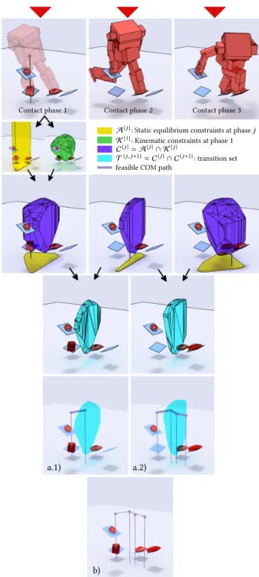
Contact phase1 Contact phase2 Contact phase3 A{j }: Static equilibrium constraints at phasej K{1}_{: Kinematic constraints at phase1}

C{j }_{= A}{j }_{∩ K}{j }

T{j, j+1}= C{j }_{∩ C}{j+1}_{: transition set}

feasible COM path

a.1) a.2)

b)

Fig. 2. Method overview. Each colored polytope corresponds to a set con-straint on the COM of the character at a specific phase of the motion.

The key idea of this paper is that in order to synthesize a plausible motion, we only need to compute a position for the

COM of the character at each transition instant. This allows us to compute a trajectory for the COM of the character extremely rapidly. Our problem is thus the following: given a set of contact phases as inputs, how should we generate a COM trajectory that will result in a plausible whole-body motion?

We illustrate our approach using Figure 2. In the first row, we can see an example of input to our method. A sequence of three contact phases is considered. This sequence describes a motion where the character moves forward using its right foot. In phase one both feet and the right arm of the character are in contact; in phase two the right foot is lifted; in phase 3 the right foot is in contact at a new location. Our method takes as inputs the contact locations at each phase, and the COM position of the character at the beginning (purple sphere), and possibly the end. Given these inputs, our method outputs a trajectory for the COM of the character, later used to generate a whole-body motion.

3.2 Transition constraints for contact phases

To define what a transition point is, we determine how the contact locations uniquely constrain the position of the COM at each phase. These constraints are formulated as 3D objects (polytopes) shown in the second row of Figure 2. Each color refers to a different kind of constraint, yellow for equilibrium (Section 4.1), green for kinematic (Section 4.2) constraints: any COM position included in a polytope respects the constraints associated to it. Since the constraints are independent, the set of COM positions that respects all these con-straints is simply the intersection of the green and yellow polytopes, shown in purple in the third row of Figure 2.

The transition instant between two contact phases is further constrained, because at this precise moment the constraints of both contact phases must be respected. The feasible transition set for the COM is thus obtained by intersecting the purple polytopes of both contact phases. This results in the blue polytopes in the fourth row of Figure 2. Any COM position included in the blue polytope is thus a candidate transition point (Section 5).

3.3 Computing a feasible COM trajectory from transition points

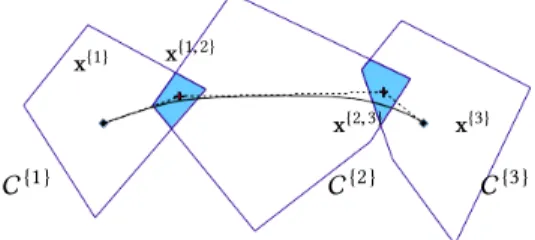
From a given COM position in contact phase 1, to reach contact phase 2 we simply need to select a transition point in the associated blue polytope (thus belonging to both phases 1 and 2), and consider the straight line between these points (Figure 2 - a.1)). We choose to deal only with convex objects, therefore in Section 5.2 we show that the straight line corresponds to a feasible trajectory (under the right time parametrization). We can then apply the same procedure to reach phase 3 from the new position, and from there a desired final position (Figure 2 - a.2)).

The resulting trajectory, while feasible, is subject to restrictive equilibrium constraints, which constrain the character to move slowly, while the Center Of Mass follows an unnatural and sharp polyline. To obtain a more dynamic trajectory, we approximate the exact polyline with a smooth Bezier curve. The design of the curve exploits the convexity properties of a Bezier curves, in such a way that the kinematic constraints are preserved. However, the price

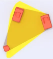
Fig. 3. Orthographic view of effector positions in contact at different heights (in red: 2 feet and one hand). In general, the convex hull (transparent grey) of the contact points is not equivalent to the admissible region for COM positions allowing for static equilibrium (yellow).

to pay for the smoothness is a small violation of the dynamic con-straints. We subjectively believe that this tradeoff is advantageous regarding the quality of the results we obtain. In Section 6, we dis-cuss the relaxation of such constraints and the generation of the Bezier curve to generate more dynamic motions (Figure 2 - b)).

4 FORMULATION OF THE TRANSITION PROBLEM

In this Section, we formulate a set of dynamic (Section 4.1) and kinematic (Section 4.2) linear constraints that define the transition problem in the quasi-static case. We use them in the following Sections to define our contributions.

4.1 Equilibrium constraints

We use a standard approach to formulate the equilibrium constraints. In the remainder of this paper, we say that a COM position or tra-jectory is equilibrium feasible if it respects the laws of centroidal dynamics given the active contact constraints. Several approaches verify equilibrium feasibility by simply verifying that the COM lies above the convex hull of the contact points projected on the ground (z = 0, where z is the height with respect to the ground). This model is valid for coplanar, almost flat contacts, and only in the quasi-static case. It does not hold in the general case [Del Prete et al. 2016]. For instance when the contacts are non-coplanar, Figure 3 illustrates that the set of admissible 2D COM positions such that the robot can be in static equilibrium has a different shape. The general formula-tion, for a given configuration withnc+ 1 contacts, is derived from the Newton-Euler equations [Qiu et al. 2011]:

H(µ0. . . µn_c, p0. . . pn_c)w ≤ h(µ0. . . µn_c, p0. . . pn_c) w = " m(¨c − g) mc × (¨c − g) + ˙L # (1) where :

• _{c, ˙c, ¨c ∈ R}3are the COM position, velocity and acceleration; •m ∈ R is the mass of the avatar;

• µi _{∈ R, 0 ≤ i ≤ nc}is the friction coefficient at the i-th contact point (we use linearized friction cones with 4 generating rays in our experiments);

• g=f0 0 −9.81gT is the gravity vector;

• ˙_{L ∈ R}3is the rate of change of angular momentum (at c). • pi ∈ R3, 0 ≤ i ≤ ncis the position of the i-th contact point.

• H and h are respectively a matrix and a vector uniquely de-fined by the piandµi [Del Prete et al. 2016].

All terms are expressed in the world reference frame.

For the moment, we will focus on the quasi-static case, where the acceleration and angular momentum are negligible. Thus w is simplified to: w= " −mg mg × c # This allows us to rewrite (1) as a function of c:

mH[:, 3:6]ˆg | {z } A c ≤ h+ mH[:, 0:3]g | {z } a (2)

where ˆg is the skew symmetric matrix of g. For each phasej, there exists a convex quasi-static polytope A{j }: {c, A{j }c ≤ a{j }}, inde-pendent ofz, illustrated by the yellow projections in Figure 2.

4.2 Kinematic constraints approximation

Given a set of 6D contact constraints, as well as the collision volumes and joint limits of the avatar, we want to express the space of feasible 3D COM positions kinematically feasible. We approximate this space with a polytope formulation, computed offline as follows. For a given effector frame ri, we sample offline an arbitrary large number of whole-body configurations (e.g. 106). For those that are collision free, we store the resulting COM position expressed in the frame ri. We then compute the convex hull Kiencompassing all these points. This convex hull is a polytope, expressed as a set of linear inequalities:

ri_{c ∈ Ki⇔}ri_Kiri_{c ≤}ri_{ki (3)}

with all variables expressed in the effector frame.

Finally, the constraints applying to a set ofncactive contacts are computed under the hypothesis of variable independence. This allows us to write

W_{c feasible ⇔ ∀i = 0 . . . nc,}W_KiW_{c ≤}W_ki

with all variables being expressed in the world frameW . This is equivalent to stacking all the constraints that define a polytope K= Tnc

i=0Ki:

W_{c feasible ⇔}W_KW_{c ≤}W_{k (4)} In the remainder of this paper we omit theW superscript and assume all variables are expressed in world coordinates. For each phasej, we can thus define a convex kinematic feasibility polytope K{j }: {c, K{j }c ≤ k{j }}, illustrated by the green polytope for phase 1 in Figure 2.

The key to the efficiency of our method is to maintain the straints applying to the COM convex. While the quasi-static con-straints are exact, Eq. (4) is subject to two approximations. They are discussed in details in Section 8.2, but are described here so that the reader bears them in mind in the remainder of the paper. First, the convex hull of Eq. (3) does not guarantee that all the points belonging to the hull are actually feasible, because of the joint limit constraints.

Then, the second approximation comes from the variable in-dependence hypothesis. Let us assume that there exists a whole

x{1}

x{1, 2}

x{2}

C{2} C{1}

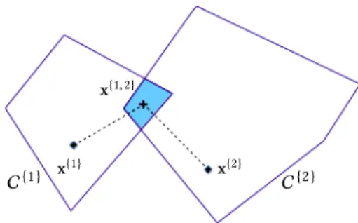
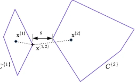
Fig. 4. 2D illustration of the transition feasibility problem. Given x{1}_and

x{2}_{, find a transition point x}{1, 2}_{in the blue polytope (if it exists). The purple}

polygons are the admissible COM positions for contact phases 1 and 2.

body-configuration such that a contact constraint for the left foot is satisfied, of COM position c. Similarly, let us assume that there exists a whole body-configuration such that a contact constraint for the right foot is satisfied, of COM position c as well. The hy-pothesis of variable independence states that there exists a whole body-configuration of COM position c, which satisfies both contact constraints. This is false in general, and problematic in practice.

While these approximations can be handled in practice, the the-oretical limitations of our work lie here. In the remainder of the paper, each time we will mention kinematically feasibility, we will refer to the Eq. (4), rather than the original problem.

4.3 Definition of the transition problem

We consider two consecutive contact phases in a motion, which differ either by a contact creation or a contact removal (Figure 2 - first row). We develop the latter case (Figure 2 - phases 1 and 2), while the first one can be straightforwardly mirrored from the following reasoning. A state x= (c, ˙c, ¨c) describes a COM position, velocity and acceleration for an avatar. For notation efficiency, we denote x{j }= (c{j }, ˙c{j }, ¨c{j })a state x that satisfies the constraints of contact phasej. We consider the issue of finding a kinematically and equilibrium feasible COM trajectory allowing to go from a state compatible with the first phase to a state compatible with the second phase, named x{1}and x{2}.

5 CONTRIBUTION 1: SOLVING THE TRANSITION PROBLEM IN THE QUASI-STATIC CASE

5.1 Finding a transition point

For the moment, because we are in the quasi-static case, we assume ˙c= ¨c = 0 for all states. In this case, the problem is schematically illustrated in Figure 4.

For a quasi-static solution to exist, a necessary condition is the existence of a transition state x{1, 2}such that the constraints of both phases are respected at c{1, 2}. In Figure 2 (fourth row) as in Figure 4, this is equivalent to proving that the blue polytope T{j, j+1}is not empty.

We observe that the kinematic constraints of phase 1 are included in the kinematic constraints of phase 2, while the equilibrium con-straints of phase 2 are included in those of phase 1. Thus, we only need c{1, 2}to be kinematically feasible regarding the constraints of

x{1} s x{2} x{1, 2}

C{2} C{1}

Fig. 5. There is no solution to this transition problem. However we can select the transition point so as to minimize the violation of the quasi-static constraint, while the kinematic constraint is always satisfied.

the first phase, and equilibrium feasible regarding the constraints of the second phase.

Finding a valid c{1, 2}can thus be computed by solving the fol-lowing Linear Program (LP):

find c{1, 2}∈ R3 s. t. A{2}c{1, 2}≤a{2}

K{1}c{1, 2} ≤k{1}

(5)

Solving (5) is enough to prove whether a solution exists. However, in our experiments we prefer the following Quadratic Program (QP) formulation: find "c {1, 2} s # ∈ R4 minimize ∥c{1, 2}−c{1}∥+ w∥s∥ s. t. A{2}c{1, 2}−1s ≤ a{2} K{1}c{1, 2}≤k{1} (6)

wherew ∈ R+ is a user defined weighting variable, and 1 is a vector of size a{2}filled with ones. The introduction of the slack variables guarantees that the method will always return a solution, guaranteed to be kinematically feasible, even if no static solution exists (in which cases ≥ 0, see Figure 5). This is interesting for computer graphics applications, because it makes it possible to always present a result (with a minimal violation of the constraints if required), rather than simply failing. Using a largew (we set it to 1000) guarantees a static solution will be chosen if it exists.

The introduction of a quadratic cost function allows us to select a transition point as close as possible to c{1}, resulting in shorter COM trajectories, which we subjectively found more plausible. In Sec-tion 7.3 we discuss how we can obtain varied results by modifying this cost function.

5.2 Generating a COM trajectory

Considering two states x{1} = (c{1}, 0, 0) and x{2} = (c{2}, 0, 0), as well as a feasible transition state x{1, 2}= (c{1, 2}, 0, 0), we now make the critical observation that the polyline c{1}c{1, 2}c{2}is both kinematically and equilibrium feasible (Figure 2 - a and 4). The proof is straightforward.

Both c{1}and c{1, 2}respect the constraints of phase 1. The set of constraints of phase 1 is a convex polytope. By convexity, any point in the segment c{1}c{1, 2}respects the constraints of phase 1. Therefore, c{1}c{1, 2}is kinematically and equilibrium feasible. □ The same reasoning applies to c{1, 2}and c{2}, thus the polyline c{1}c{1, 2}c{2}is both kinematically and equilibrium feasible. This means that, in the quasi-static case, with a simple call to a low dimensional QP, we are able to compute a feasible trajectory.

We stress the fact that this trajectory does not provide a time parametrization, because of its quasi-static nature: as long as the acceleration remains negligible, the motion is feasible. Formally, if s(t ), t ∈ [0, 1] is a constant-velocity time parametrization of the polyline, ∃ϵ (t ) such that the trajectory c(t ) = s(ϵ(t)) is equilibrium (and kinematically) feasible. For c(t ) to be feasible, ϵ (t ) must be such that each transition point of the polyline is reached with a velocity of 0. We say that s(t ) is ϵ feasible.

6 CONTRIBUTION 2: RELAXING THE QUASI-STATIC CASE (2PAC)

The quasi-static solution computes COM trajectories that are poly-lines, alternating between straight lines and sharp turns at the tran-sition points. This results in unnatural looking motions, although physically accurate. Our objective is now to slightly relax the quasi-static constraint to obtain more subjectively appealing trajectories. We propose to use Bezier curves, because they can approximate arbitrarily well any smooth trajectory, and present a relevant prop-erty: any point in a Bezier curve belongs to the convex hull of its control points. The transition points will be used as control points for the curve.

6.1 A remainder on Bezier curves for trajectory generation

We define a COM trajectory connecting two states x{1}and x{l }, (wherel > 1) as a Bezier curve c(t ) of degree n ≥ 5:

c(t ) = n X k=0 Bn k(t )Pk (7) where theBn_kare the Bernstein polynomials and the Pkare control points. All the curves that we use comprise at least 6 control points to ensure that the following constraints are verified:

• P0= c{1}and Pn = c{l }guarantee that the trajectory starts and ends at the desired locations;

• P1= ˙c{1}/n + P0and Pn−1= Pn−˙c{l }/n guarantee that the trajectory initial and final velocities are respected;

• P2= ¨c{1}/(n(n − 1)) + 2P1−P0and

Pn−2= ¨c{l }/(n(n − 1)) + 2Pn−1−Pnguarantee that the tra-jectory initial and final accelerations are respected.

We could simplify these equations since the velocities and ac-celeration are 0, but we use this general formulation because this constraint will be removed in Section 6.4.1.

6.2 Using one or two transition points as control points.

In this first case, we relax the quasi-static constraint to generate smooth trajectories, while we guarantee to preserve kinematic feasi-bility. We consider an additional control point to our nominal Bezier curve:

x{1} x{1, 2}

x{2, 3} _x{3}

C{3} C{2}

C{1}

Fig. 6. A polyline COM trajectory is approximated with a smooth Bezier curve, where the transition points become attractors points, used as control points of the Bezier curve. The curve lies in the convex hull of the control points. c(t ) = X k ∈ {0, 1, 2, 4, 5, 6} B6 k(t )Pk+ B 6 3(t )c{1, 2} (8) This curve uses a transition point as a control point that “at-tracts” the trajectory towards it, and as such, is an approximation of the polyline c{1}c{1, 2}c{2}. In the remainder, we make a semantic distinction between a transition point and an attractor point: a transition point is a point reached by a polyline COM trajectory (Figure 4). An attractor point is a transition point used as a control point of a Bezier curve describing a COM trajectory. It is thus never reached by definition (Figure 6).

The advantage of using Bezier curves is that we can guarantee that the curve (8) is kinematically feasible everywhere.

The demonstration is straightforward: Let us assume that a con-tact is removed from phase 1 to phase 2, as in Figure 2 (a mirror reasoning applies for the contact added between phases 2 and 3). In this case, all the control points of c(t ) belong to the kinematic polytope K2. By definition of a Bezier curve, c(t ) is entirely in-cluded in K2, and thus respects the kinematic constraints of phase 2. Moreover, a portion of c(t ) is kinematically feasible for phase 1 (because at least c{1}respects this constraint). Therefore, there ex-ists a contact transition time that makes c(t ) kinematically feasible, under the assumption that our approximated kinematic constraints are exact.□

With the same reasoning, it is possible to generate a smoother Bezier curve with the same guarantees for three consecutive phases, if and only if a contact is removed in phase 1, and another is added in phase 3: c(t ) = X k ∈ {0, 1, 2, 5, 6, 7} B7 k(t )Pi + B 7 3(t )c{1, 2}+ B74(t )c{2, 3} (9)

6.3 Using m transition points as control points.

To generate even smoother trajectories, we can consider using at-tractor points form + 1 consecutive phases:

c(t ) = Bm 0 (t )c{1}+ m−1 X i=1 Bm i (t )c{i,i+1}+ Bmm(t )c{m } (10) In this general case we lose all theoretical guarantees of feasibil-ity. However, we can iteratively construct a curve that ultimately converges to a feasible trajectory.

Let s(t ), t ∈ [0, 1] be a ϵ feasible parametrization of the polyline c{1}c{1, 2}. . . c{m−1,m }c{m }. The curve c(t ) = n X k=0 s k n ! Bn k(t ) (11) converges towards s(t ) as n increases, according to the Weierstrass Approximation Theorem [Weierstrass 1885].

It is thus possible to generate a curve of arbitrary degreen, and increasen until the required constraints are satisfied, with the guar-antee to converge towards the original feasible solution. The attrac-tor points thus drive the COM trajecattrac-tory towards the quasi-static solution, without exactly reaching it.

6.4 The 2 Points Attractors for COM trajectories method (2PAC)

After presenting the theory behind our method, we propose a con-crete implementation, which is the one we used to generate our results. In summary, we use a maximum number of 2 attractor points for generating Bezier curves to ensure kinematic feasibility, and we use a sliding window to connect consecutive curves, so as to avoid stopping along the motion.

Generating a COM trajectory over a window of 2 (respectively 3) contact phases results in a Bezier curve comprising 1 (respectively 2) attractor point(s), with the guarantee that the computed trajectory is always kinematically feasible. Considering simultaneously more than 3 contact phases requires to introduce an iterative approach to progressively introduce new attractor points until a feasible trajec-tory is obtained. However, as more contact phases are considered, the resulting trajectory becomes smoother. Because we ultimately target real time applications, we choose a maximum window size of 3 contact phases for trajectory generation.

6.4.1 Using a sliding window to generate a smooth trajectory over many contact phases. Each trajectory c(t ) is created such that the terminal velocity ˙c(1) is null. This results in the character stopping completely after each contact creation, a limitation shared with other methods such as [Naderi et al. 2017].

However in our case, we can easily remove this constraint thanks to the connectivity property of Bezier curves, using a sliding window. Let us consider again the example from Figure 2, extended with a fourth contact phase where the hand contact is removed. We thus look for a COM trajectory connecting a state x{1}to a state x{4}, given {x{j }, j = 1 . . . 4}. In this case we use the following scheme:

• Compute a trajectory c1(t ) for phases 1 to 3 that connects x{1}to x{3};

• Chooseu ∈ [0, 1] such that c1(u) ∈ K{3}and ˙c1(u) , 0, and define x∗{3}= (c1(u), ˙c1(u), ¨c1(u));

• Compute a trajectory c2(t ) for phases 3 to 4 that connects x∗{3}to x{4};

• The concatenation of the curves is a kinematically feasible Bezier curve, by construction of the state x∗{3}.

We can iteratively repeat this process for arbitrary long contact sequences: generate a kinematically feasible trajectory for the first 2 or 3 contact phases; select a point in the trajectory that respects the kinematic constraints of the last contact phase reached; generate

x{1}

x{2} _C{2} C{1}

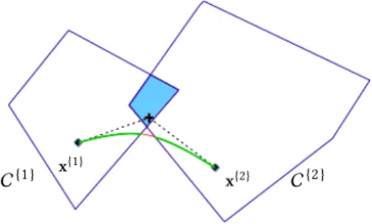
Fig. 7. With 2PAC, the quasi-static constraints can be violated on a small portion of the COM trajectory (red part of the curve). The kinematic con-straints are always respected.

from this point a kinematically feasible trajectory for the 2 or 3 next contact phases, and concatenate it with the previous one; repeat until the last contact phase is reached.

6.4.2 Dynamic validation and time parametrization of the tra-jectory. The trajectory obtained with 2-PAC is guaranteed to be kinematically feasible. But what about the quasi-static constraints ? Because the transition points are never reached, there is no guaran-tee that the COM trajectory intersects the transition set. In Figure 7, the red part of the trajectory violates the quasi-static constraint. This happens because the kinematic constraints impose to break a contact too soon, or to create the contact too late. We empirically quantify this violation in Section 8.2.

Finally, the Bezier curves are defined on a normalized interval [0, 1]. It is thus necessary to find a time parametrization of the tra-jectory. To respect the quasi-static constraint, we should compute an accurate parametrizations(t ) (or just choose an arbitrary large total duration). Here again, we prefer a trade-off between dynamic accuracy and subjective quality of the resulting motion. We empir-ically computes(t ) by scaling the time t by a weighted distance between the start and goal whole-body configurations. In Section 8.2, we comment on the validity of this approach and show that the dynamics is respected along most of the generated trajectories.

7 APPLICATION: GENERATION OF MULTI CONTACT MOTIONS

To be able to compute the COM trajectories, our method requires as input a list of states x{j }. Thus, to demonstrate our method, we integrate it within a framework for multi contact locomotion.

Figure 8 illustrates the work flow.

7.1 Work flow description

To generate the states, we use an open source procedural contact-planner [Tonneau et al. 2015]. Given a desired start and goal COM positions, the contact planner is able to compute a discrete sequence of whole-body contact configurations that describe the motion, such that at most one contact is broken and another contact is added between two consecutive configurations.

We consider two uses cases for the planner:

desired start / goal COM positions Contact Planner Sequence of whole-body contact configurations Our method (2PAC) COM trajectory Whole body motion generator Final motion

Fig. 8. Workflow of our overall system. The rounded rectangles are the inputs and outputs of the framework. The unbounded text refer to internal inputs / outputs used by the three main blocks (sharp rectangles). The whole body motion generator considers as inputs the COM trajectory, but also the initial and goal whole body configurations of the character.

• case 1: one contact planning. In this interactive context we are only interested in computing the next step. The goal con-figuration is unknown. A random process (or a user) selects a direction of locomotion, and a target contact phase reachable from the current phase in that direction. The planner then generates a collision free, whole-body configuration in static equilibrium that meets the constraints;

• case 2: contact sequence planning. The planner computes a sequence of contact phases and configurations allowing to reach a user defined goal configuration.

In the first case, the environment (or another character) geometry can be discretely updated between each step, while in the second case the contact sequence is planned on a static environment. In both cases, our method then generates a COM trajectory, used by a dedicated motion generator to synthesize the final motion.

7.2 Whole body motion generation

To generate a whole-body motion given a user defined time parame-trization of the COM trajectory and contact constraints, we use a generalized inverse kinematics solver. The method first computes a whole-body motion that follows the given COM trajectory and satisfies the contact constraints [Baerlocher and Boulic 2004].

However, because our formulation does not take into account these environmental constraints, it is possible that a computed COM trajectory defines an unfeasible problem (ie there does not exist a whole-body motion which is both collision free and satisfies the

COM constraints). Our planner provides empirical guarantees that a solution exists, and thus we use a local adaptation scheme to try to compensate for these collisions. However we stress the fact that this local adaptation is not guaranteed to converge. The accurate handling of collision constraints with centroidal approaches remains an open problem that we do not claim to solve in this paper.

We consider two types of collisions. If a limb is in collision, a constraint-based RRT planner is used on the joints of the limb to look for a collision free motion for the limb, while preserving the contact and COM constraints. This solver is a feature of our motion planner, and its details can be found in [Mirabel et al. 2016].

Otherwise, if the root is in collision at an instantt, with a pen-etration greater than a user defined value (we use 5cm in our ex-periments), we assume that the computed COM trajectory is not feasible (If the penetration is lesser than the threshold, we assume that moving the free limbs is sufficient to avoid the collision). In such cases, we replace the transition point ccl osethat is the closest to the first collision point in the trajectory. To do so we consider the first obstacle in collision with the root, and its surface normal ns. ns gives a repulsion direction. A new transition point cnew is com-puted as cnew = ccl ose+ αns, whereα is given by the penetration distance between the root and the obstacle. The transition points locations are updated iteratively until either a collision free solution for the root is found, or a computed cnew no longer respects its phase constraints.

In both cases, we use a user-defined time out value after which the best motion found is returned. It thus appears that when the root is in collision with the environment, our collision avoidance algorithm is not complete, because the approach is local. However, in our experiments this rarely occurred, because the contact planner guarantees that the segment connecting the root poses of two suc-cessive key postures is collision free. However, we cannot guarantee that a collision free solution be found if it exists. This is a limitation shared with all existing multi contact approaches, although our experiments demonstrate that our method is able to handle severely cluttered cases.

7.3 Scenarios

The companion video 1 shows the versatility of our method, in the variety of situations it addresses. We use four characters: two humanoids (including the HRP-2 robot), a quadruped, and a six-limbed creature (Figure 1).

Our main scenario is interactive and matches the first use case. The humanoid and the quadruped play a variant of a game of Twister (http://cpc.cx/k5j): at each turn, an effector is selected to either create a contact or break it (Figure 1 - Left). The contact planner computes a state that satisfies the new constraint, and our method computes the motion to reach the state, by taking into account the bodies of the other character. If no such solution is found, a new effector is randomly selected. This scenario illustrates the ability of our method to compute motions in close interaction while avoiding collisions. Another scenario shows a humanoid avatar sitting or standing on a chair, in two cluttered environments (Figure 1 - Middle). The scenario demonstrates the strong advantage of combining a contact planner with our method: variations of the same motion can be obtained automatically and almost instantly to adapt to new scenes,

in a way different from classical motion editing approaches, because the contact phases differ between the different iterations.

In a third scenario a creature with six limbs, or a humanoid, climbs along a set of cubic obstacles (Figure 1 - Right). The same scenario is addressed for both creatures without requiring specific heuristics, tuning, or discretization of the environment.

We also demonstrate more dynamic motions in simpler environ-ments, with the humanoid character crossing a set of uneven stairs, or the quadruped climbing a steep hill. These scenarios demonstrate the ability of our planner to handle such cases, although less generic physics-based methods are able to generate more appealing results in those specific cases.

User parametrization of the motion. Our approach leaves room for artistic authoring of the motions, as demonstrated in our remaining scenarios.

To achieve this, one option is to manually select relevant tran-sition / attractor points. This is demonstrated in a scenario where 3 different motions are obtained between the same two contacts phases. The variation is obtained through the manual displacement of the transition points by a user along the z axis. Since they attract the COM trajectory towards them, the transition points are an in-tuitive tool to control the trajectory. The 3D representation of the admissible positions for a transition point allows the user to easily determine where to put such points.

Another option is to set up user-defined cost functions that will be used to automatically compute the trajectories. To illustrate the versatility of our method, we designed simple cost functions that resulted in the “silly walks” (http://cpc.cx/lYM) we present with the humanoid robot HRP-2 in two different setups. We obtain a “tired” motion by minimizing the distance traveled at each step, or a “groovy” motion by maximizing the lateral variation during the motion. We also constrain the COM to be as far to the right side of the robot as possible, or as close as possible to the ground, to generate more “cartoonesque” motions. The advantage of such cost functions is that they do not require to manually define new control points on new environments, as illustrated in the first companion video.

8 EVALUATION OF THE METHOD

In this section we provide and analyze some numbers, first regard-ing the computational performance of the method, then regardregard-ing the errors introduced in our formulation by the linearization (ap-proximation) of the kinematic constraints, and finally, regarding the physics violations that may occur upon using 2PAC.

8.1 Time performance

We present the times measured upon computation of a COM trajec-tory for an avatar, which is the main contribution of the paper. For convenience, we also provide the indicative times used to generate the results demonstrated in the companion video, but we refer the reader to [Tonneau et al. 2018] for an extensive analysis of the plan-ner (times and success rates). The performance is measured with an Intel Xeon CPU E5-1630 v3 at 3.70GHz, with a single threaded python implementation.

number of active contacts Constraint computation time (ms) 1 0.157 2 2.11 3 5.14 4 14.0 5 33.7 6 68.19

Table 2. Average computation time for the dynamic constraints of a contact phase, where each contact is described by four contact points.

8.1.1 Computation time of the COM trajectory. The only signif-icant component of the time spent in the trajectory generation is the computation of the transition points (in the case of 2PAC, the generation of a Bezier curve is neglectable). This time is decomposed between the time required to compute the dynamic constraints of a given problem (the kinematic constraints are computed offline), and the time to solve QP (6). Table 2 presents the average compu-tation time for the constraints, depending on the number of active contacts.

The time to solve the QP, thus finding a transition point between two phases, averages to 0.2 ms, independently from the number of active contacts at each phase. Therefore, in a nominal use of 2PAC for a quadruped, at most 150 ms are required to compute a COM trajectory having 10 contact phases. This time is at least one order of magnitude faster than any existing method (Table 1).

A more computationally efficient yet equivalent problem. The com-putation time required to compute the dynamic inequality con-straints of Equation (2) increases cubicly according to Table 2. To further alleviate the computational burden, it is possible to use an equivalent and straightforward formulation of the dynamic con-straints of Eq. (2). This formulation does not express the concon-straints with linear inequalities, but rather as the following equality con-straint, given by [Del Prete et al. 2016]:

" I3 . . . I3 ˆp0 . . . ˆpnc # V | {z } G β, ="03×3 mˆg # | {z } D c+"−mg 0 # | {z } d (12) where:

• _{ˆx ∈ R}3×3is the cross-product matrix associated to x; • _{V ∈ R}3nc ×4ncis the matrix containing the diagonally stacked

generating rays of the friction cone of each contact point; • β ∈ R4ncis a positive vector variable.

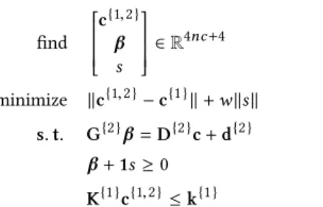
Eq. (12) and Eq.(2) are strictly equivalent as they define the same static equilibrium constraints. So far we used the latter because the linear constraints are more intuitive to handle in our framework, but if the 3D visualization of the constraints is not required, using (12) is faster. We can thus define a QP strictly equivalent to (6):

find        c{1, 2} β s        ∈ R4nc+4 minimize ∥c{1, 2}−c{1}∥+ w ∥s∥ s. t. G{2}β = D{2}c+ d{2} β + 1s ≥ 0 K{1}c{1, 2}≤k{1} (13)

Under this new formulation, the only relevant time is now the resolution of the QP itself, because the constraints are computed straightforwardly. Solving this QP requires less than 1 ms in the worst case (6 contacts in our tests), which reduces the computational time to less than 10 ms for a sequence of 10 contacts phases. We can thus conclude that the method is compatible with real time applications.

Computation time for the complete framework. Regarding Figure 8, the other time consuming operations are the computation of an input contact sequence, and the generation of the whole-body mo-tion from the COM trajectory. In all the scenarios presented, the planning time for the contact sequence is less than a second in the worst case. We refer the reader to [Tonneau et al. 2018] for a detailed analysis on the impact of the complexity of the scene with respect to the planning time.

The actual generation of the whole-body motion is strongly de-pendent on the complexity of the environment, from the standing up / sitting down scenarios (100ms for one second of animation on average, including planning) to the twister scenario (2s for one sec-ond on average). The total time to generate a motion comprising 10 contact creations thus never exceeds a few seconds, with an average time of about one second.

8.1.2 Comparison with the state of the art.

Computation time of the COM trajectory. Regarding the time to compute the COM trajectory, our method compares favorably to the fastest existing approaches [Carpentier et al. 2016; Herzog et al. 2015], which take on average several hundreds of milliseconds with-out guarantee of convergence, making them unsuited for a robust real time graphical application, contrary to our approach.

Computation time for the complete framework. Comparing our results with other approaches is not trivial, because the inputs and outputs differ between each method. For instance [Mordatch et al. 2012] compute a COM trajectory simultaneously with the contact locations, but the inverse kinematics is generated afterwards and does not consider collisions and joint limits; [Naderi et al. 2017] address the complete problem, but consider an unordered set of contact points as inputs; our planner computes a discretized set of contacts postures used as inputs. For these reasons and because detailed computation times are not always available, we cannot pro-vide an extensive comparison of the performance of the methods. Still, we can compare the order of magnitudes of the computation times obtained with respect to the literature. Table 1 suggests that our framework performs better, or at least not worse, with respect to the literature, while we address severely cluttered scenarios that

scenario Success rate chairs 100 % silly walks 100 % stairs 97 % steep slope 85 % twister 82 % climbing (no quasi-static) 56 %

Table 3. Validation of the dynamics for COM trajectories generated with 2PAC

have not been demonstrated by the other methods. This comparison shows that 2PAC can be integrated with existing animation frame-works to obtain a complete solution faster than existing approaches.

8.2 Accuracy of the method

Dynamic accuracy. Our equilibrium constraint is exact in the quasi-static case, and a feasible solution will always be found if it exists. In this nominal case, the generated trajectories are thus always physically accurate.

With 2PAC, this is not the case anymore, since the dynamic con-straints are relaxed. In the first companion video, we included some examples where such violation occurs. To evaluate the accuracy of the trajectories, we used the following protocol. For each scenario we consider, we discretize the obtained COM trajectories, and at each discretization point, we use equation (1) to verify the dynamic validity. This allows us to compute the ratio of dynamically consis-tent trajectories, summarized in Table 3. As we can see, the more dynamic the motion becomes, the less accurate 2PAC is. However, the ratio of validated points is high, except for the climbing scenario. In this scenario, there is no quasi-static solution that would allow the character to climb the wall. As excepted in such case, 2PAC finds a solution where the parameters of QP (6) is not zero, which indi-cates a violation. This is also the case for the steep slope scenario, as well as for the some transitions in the twister scenario.

Kinematic accuracy. A limitation of our approach lies in the hy-pothesis of independence, used to compute the kinematic feasibility polytope as the intersection of the kinematic constraints associated with each active contact. As a result the kinematic constraint is not exact, but only approximated. In this paragraph we show that the hypothesis is strongly invalidated in the general case when the number of contacts increase, but that it remains efficient in realistic scenarios.

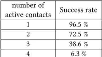
To test the validity of the hypothesis in the general case, we con-sidered the humanoid, which is the most kinematically constrained character. We then counted over a large set of scenarios, the number of false positives resulting from the hypothesis of independence. In other words, we determined the percentage of times where no whole-body configuration existed that allowed to satisfy the contact constraints while positioning the COM at a given location. We used the following protocol.

We randomly sampled 1000 contact configurations from the test environments used in our experiments, equally distributed between 1, 2, 3 and 4 active contacts. For each set of contacts, we randomly

number of

active contacts Success rate 1 96.5 % 2 72.5 % 3 38.6 % 4 6.3 %

Table 4. Validation of the kinematic constraint for the humanoid character, depending on the number of contacts active, with an uniform sampling.

sampled 1000 COM positions included in the kinematic constraints polytope. We then tried to generate as many whole-body postures satisfying the contact constraints while reaching the sampled COM, and evaluated the success rate of this operation (by accounting for internal collisions and joint limits violations). Table 4 summarizes the results.

As expected, the number of false positives increases significantly with the number of contacts, and rather dramatically after 3 con-tacts, highlighting the fact that the independence hypothesis is false. However, these numbers are not representative of the kinematic accuracy of our method. Indeed, as opposed to this protocol, with 2PAC the kinematic constraints polytope is not uniformly spanned: the computed COM trajectories follow a path connecting two kine-matically valid and relatively close configurations, which satisfy a quasi-static constraint that constrains the COM to lie above the contacts.

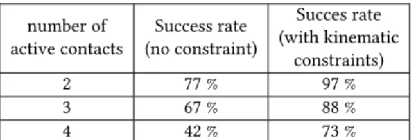
To verify the validity of the hypothesis in our scenarios, we mea-sured the kinematic feasibility validation as follows. We randomly generated 1000 feasible transition problems, over the scenes used in our scenarios. For each problem, we computed a transition point, and verified whether we were able to generate a whole-body mo-tion along the complete COM trajectory. If anywhere along the trajectory, the inverse kinematics failed, we counted the scenario as a failure. Conversely, if the whole trajectory was successfully extended as a whole body motion, we counted the scenario as a suc-cess. We performed the analysis in two different contexts: one when the kinematic constraints were active, and the other one where no kinematic constraints were used. Table 5 summarizes the results. We observe that in our scenarios the kinematic constraints increase significantly the success rate, despite being less and less accurate as the number of active contacts grow. If we consider the same protocol for all creatures used in our demonstrations, the success rate averages to 93 %. This higher number is explained by the fact that the humanoid is the most constrained kinematically. In our method, when a false positive is encountered, we treat the issue as if there was a collision between the root of the character and the environment, that is we translate the position of the transition point, in the direction towards the center of the polytope.

8.3 Failure cases

There are cases where our approach will not be able to find a solution within a reasonable time limit. The method will fail because it won’t be able to provide a collision free whole-body motion, or because it won’t be able to provide a motion that satisfies the kinematic constraints of the character. Whether the given problem is feasible

number of active contacts Success rate (no constraint) Succes rate (with kinematic constraints) 2 77 % 97 % 3 67 % 88 % 4 42 % 73 %

Table 5. Validation of the kinematic constraint for the humanoid character on the scenarios we consider. First column indicates the success rate without the constraint, second column indicates the success rate with the kinematic constraints taken into account.

or not in such cases is impossible to know. In our experiments, the main problem comes from the collisions with the environment, which impose non-convex constraints that are only locally handled by our method.

From a practical point of view, one option is to relax these con-straints to allow small penetrations or joint limit violations [Kang and Lee 2017; Mordatch et al. 2012].

9 DISCUSSION AND FUTURE WORK

In this paper we presented 2PAC, a method for computing COM trajectories for legged characters in multi contact situations, com-bined with an existing contact planning approach. This method provides a fully automated framework for synthesizing multi con-tact movements for arbitrary legged characters and environments, as demonstrated by our results. In this Section we discuss the im-mediate implications of our method, as well as the perspectives it opens in terms of physics-based computer animation.

A procedural approach allowing for artistic control

As of today, few physics-based methods are used for character ani-mation in the industry, for two main reasons (in our opinion). Firstly, these methods are often complex and hard to integrate within ex-isting frameworks, and sometimes computationally expensive. Sec-ondly, they do not provide flexibility to the artist, who often loses control of the animation. 2PAC is fast and simple to integrate within existing animation systems. Indeed, although we demonstrate a fully automatic approach, it could straightforwardly be used in co-ordination with motion capture based or artist edited animation systems. In such a case the whole-body generator would solve a constrained optimization problem to limit the deformation of the reference motion, for instance as in [Tonneau et al. 2016].

More importantly, 2PAC also provides flexibility. Firstly because editing the results is easy through the manipulation of the transition points. The 3D representation of the constraints offers an easy way for the artist to select the transition points and time parametrization, to obtain a subjectively better motion. Secondly, because we control the COM rather than the whole-body pose, the user can easily specify additional pose constraints on the motion. In such cases where trial and error is required, the rapidity of our method is a strong asset. The efficiency of our method thus makes it interesting for both online and offline motion synthesis applications.

A step towards accurate centroidal approaches

As all existing methods using the point mass model, our method approximates the constraints that govern the whole-body motion of a character. Compared to these approaches our results demonstrate that 2PAC better approximates these constraints, while obtaining better computation times. Regarding the equilibrium of the charac-ter, we have shown that first restricting the motion to a quasi-static case before relaxing it already allows us to address a large vari-ety of problems. One exciting direction of improvement is to use the computed trajectories to warm start existing optimal control solvers [Carpentier et al. 2016; Herzog et al. 2015], with the hope that they would converge much faster to a dynamically accurate solution.

Regarding the improvement of our kinematic constraints, using learning approaches such as [Carpentier et al. 2017; Kang and Lee 2017] is a promising direction for future work, although it would require to learn the dependencies between the different limbs of the character. Another interesting option to improve the quality of the results would be to account for the torque limits of the characters at the centroidal level, using recent contributions from the robotics field [Orsolino et al. 2018].

A new approach for computing COM trajectories

The computation of a COM (or a whole-body) trajectory is usu-ally treated as a nonconvex optimization problem by procedural approaches. Handling the discontinuities induced by the contact phases in this continuous formulation in particular is one of the bot-tlenecks of the problem. Our take is completely different from this classic approach, in the sense that our formulation of the problem is discrete, since we only focus on transitions. Our work suggests that a quasi-static legged motion can be entirely defined by characterizing these discrete transition instants. Currently, our approach suffers from the quasi-static constraint, which prevents the synthesis of subjectively appealing, truly dynamic motions. We are currently focusing on removing this limitation, with encouraging preliminary results to appear in [Fernbach et al. 2018]. Additionaly, we believe that the convexity properties of Bezier curves may provide a way to address the trajectory generation problem in a continuous fashion, which could benefit to any approach, including those using non linear solvers. In particular we are excited about testing such for-mulation within the recent framework proposed by [Winkler et al. 2018]. Still, our objective remains to get rid of the non-linearity of the centroidal dynamics in the general case, and we believe that better characterizing the constraints active at the transition phases could result in a generalization of our approach to arbitrary legged locomotion. We hope to inspire more research in this direction.

10 SOURCE CODE OF OUR METHOD

The source code of 2-PAC is to be released as part of a C++ library with python bindings, under a BSD-2 license, available at