Computational studies of cation and anion ordering in cubic yttria stabilized zirconia

Computational Studies of Cat ion and

Anion

Ordering in Cubic Yttria Stabilized Zirconia

Ashley

P.

Predith

Submitted t o the Department

of Materials Science and Engineering

in partial fulfillment of the requirements for the degree of

Doctor of Philosophy

at the

MASSACHUSETTS INSTITUTE

OF

TECHNOLOGY

June 2006

@

Massachusetts Institute of Technology 2006. All rights resewed.

Author

...

w

-.7-

....-...

...

Department of Materials Science and Engineering

April

28,

2006

Certified by.

...

... .--.

-

.

;.

...

~/3/.*6'

Gerbrand Ceder

R.P.

Simmons Professor of Materials Science and Engineering

Thesis Supervisor

n

A

i.

/

...

Accepted

by

...

~~.Y.V.W.Y.-.-.~.

.

: .-. .&

. . .

.,.

Samuel Mi Allen

POSCO Professor of Physical Metallurgy

Chairperson, Department Committee on Graduate Students

' MASSACHUSElTS INSTITUTE ,' OF TECHNOLOGY

LIBRARIES

Computational Studies of Cation and Anion Ordering in

Cubic Yttria Stabilized Zirconia

by

Ashley P. Predith

Submitted t o the Department of Materials Science and Engineering on April 28, 2006, in partial fulfillment of the

requirements for the degree of Doctor of Philosophy

Abstract

The investigation of ordering and phase stability in the Zr02-Y203 system involves two sets of calculations. The first set of calculations uses the cluster expansion method. A guide t o the practical implementation of the cluster expansion outlines methods for defining a goal and choosing structures and clusters that best model the system of interest. The cluster expansion of the yttria stabilized zirconia system considers 447 configurations across the Zr02-Y203 composition range. The effec- tive cluster interact ion for pair clusters show electrostatic repulsion between anions and little interaction between cations. Triplet anion terms largely modify the en- ergy contributions of the pair terms. Separate cluster expansions using structures a t single compositions show that cation clusters become more important at high yttria composition.

The cluster expansion led t o the discovery of three previously unidentified ordered ground state structures at 25, 29, and 33

%

Y on the cubic fluorite lattice. The ground state with 33

%

Y is stable with respect to the calculated energies of monoclinic Zr02 and the Y4Zr3OI2 ground state. The ground states have the common ordering feature of yttrium and vacancies in [I 1 21 chains, and Monte Carlo simulations show that vacancy ordering upon cooling is contingent on cation ordering.

The second set of calculations consider three driving forces for order: ionic re- laxation, vacancy arrangements, and differences in Zr and cation dopant radii. Bond valence sums of fully relaxed and anion relaxed structures are nearly equal at all com- positions. In supercells of Zr02, the vacancy arrangement of the ground state with

25 % Y is more stable than arrangements maximizing the distance between vacancies or aligning vacancies in [I 1 11. Comparing the YSZ ground state with structures of the same configuration with scandium replacing yttrium shows different stable phases on the convex hull between cubic ZrOz and the dopant M 2 0 3 phase. The change in the stability of the configurations may be a result of cation radius sizes. The factors suggest that the driving forces of phase stability depend on composition.

Thesis Supervisor: Gerbrand Ceder

Acknowledgments

I first thank my advisor Gerd Ceder . His contagious enthusiasm for science was ener- gizing during the course of study. I appreciated his scientific insight and suggestions about how to analyze and approach this research.

Professors Nicola Marzari and Harry Tuller on my thesis committee had useful suggest ions and provided thoughtful discussion.

Early work on the cluster expansion of YSZ was done in collaboration with Chris Wolverton and Alex Bogicevic of Ford Motor Company. Their initial work provided a foundation for the work in this dissertation.

My work also depended on the efforts of past and current members of the research group. The ways people contributed covered the gamut from the physical acts of setting up and maintaining computer systems, t o helping sort out VASP issues, giving advice on classes, to late night camaraderie and conversations in lab. While only names are listed here, each person has a unique face and personality very much part of my time in the group: Eric Wu, Chris Marianetti, Elena Arroyo, Dane Morgan, John Reed, Dinesh Balachandran, Anton van der Ven, Stefano Curtarolo, Kristin Persson, Matteo Cococcioni, Shirley Meng, Byungchan Han, Kisuk Kang, Tim Mueller, Chris Fischer, Maria Chan, Fei Zhou, Byoungwoo Kang, Yoyo Hinuma, Thomas Maxisch, Kevin Tibbetts, Caetano Miranda, Lei Wang, Osman Okan, and Kathy Simmons.

The cluster expansion of YSZ was done with the assistance of Anton van der Ven and Tim Mueller. Tim delved in to the cluster expansion process, offering a fresh perspective and succinct approach, and Anton's stream of ideas as well as his readiness and patience in answering questions was met with gratitude by me and many others. I especially thank Kristin Persson for frank analysis of the calculations and for sharing her experience on many levels. Talking with her about the process of research has been greatly valued.

In addition to the people in lab, I was fortunate for the emotional and spiritual support of friends. The large apartment that I lived in housed many people during my time there, and my roommates made it a quirky, interesting place to come home to

after a long day at the computer. Holly Krambeck, Ben Paxton, Max Berniker, Bonna Newman, Megan Carroll, and Ayala Wineman particularly made our apartment a great place to live.

I

am thankful to many for their friendship, and

I

could not name everyone here explicitly. Doug Twisselmann, Douglas Cannon, Bruce Constantine, and Andy Mar- tinez were there from the very beginning. Elizabeth Daake, Shawn Kelly, Christina Silcox, and Joaquin Blaya joyfully celebrated holidays and events with me, and Mau- reen Long, Christine Ng, Elizabeth Basha, and

I

experimented our way through many happy dinners. Michael Steinberger enriched my experience in multiple ways. The Tech Catholic Community provided a fantastic environment in which to question, learn, and grow.

I

thank Paul Reynolds for his caring presence that was steadily felt over the years.

Throughout classes, qualifying procedures, research, teaching, nieces, and nephews, Marc Richard was with me throughout grad school. Jenny Lund was always ready for long talks on the telephone or for heading out on our next trip. Whether listening as

I

vented about things

I

was struggling with or making me laugh so that

I

literally could not walk, Maria Chan has been a genuine and indispensible friend over the past two years.

I

sincerely thank you, Maria.

Finally, my family. They each had a unique role that contributed to me finishing this dissertation, and

I

am grateful for their presence and love. Unfailingly listening, supporting, and cheering me on, my mom Patty Predith has been there every step of the way. My dad Jim Predith shares my interest in science and dared to ask more than once for an explanation of what

I

was working on. My brother and my niece Colin Predit h and Meera Kypta and my sister, brother-in-law

,

and nephew Hilary, Brad, and Brendan Smith gave me a balanced perspective on life and helped me keep an eye on the future. Thank you so much.

The words of family, friends, coworkers, and the wider community made all the difference during my time in graduate school. The path was at times solitary and difficult, at times enlightening and deeply satisfying. Having little previous knowledge of Eleanor Roosevelt, I accidentally discovered her writings and found them to be

particularly meaningful:

"The encouraging thing is that every time you meet a situation, though you may think at the time it is an impossibility.. .

,

once you have met it and lived through it you find that forever after you are freer than you ever were before ... You gain strength, courage, and confidence by every experience in which you really stop to look fear in the face ...

Courage is more exhilirating than fear and in the long run it is easier. We do not have t o become heroes overnight. Just a step at a time, meeting each thing that comes up, seeing it is not as dreadful as it appeared, discovering we have the strength to stare it down."

Contents

1 Introduction 23

1.1 Conductivity

. . .

23

1.2 Structure and phases

. . .

24

. . .

1.3 Investigations of order and phase stability 26 2 Cluster expansion implementation 27 2.1 Developing a cluster expansion

. . .

27

2.1.1 Cluster expansion background

. . .

27

2.1.2 Purpose of the cluster expansion

. . .

29

2.2 Metrics of the expansion

. . .

30

2.2.1 Root mean squared error

. . .

31

2.2.2 Cross validation score

. . .

31

2.2.3 ECIerror

. . .

31

. . .

2.2.4 Cluster expanded energy of trial structures 32

. . .

2.3 Factors for implementation 33

. . .

2.3.1 Cluster choice 34 2.3.2 Structure choice

. . .

38

2.3.3 Mathematical fitting

. . .

43

3 Cluster expansion of Zr02.Y01.5 using first principles energies 45 3.1 Expansion on coupled sublattices

. . .

45

3.2 Energies from first principles . . . 45

3.3.1 Clusters

. . .

3.3.2 ECI

. . .

3.3.3 Convex hull and monoclinic Zr02

. . .

3.4 Limiting clusters by type of ion

. . .

3.5 Limiting structures by composition

. . .

4 The ground states of YSZ .

4.1 Literature review of Zr02 YO1.S ordering

. . .

4.1.1 Relaxations and displacements

. . .

. . .

4.1.2 Vacancy position relative to Y and Zr

. . .

4.1.3 Microscopic order

. . .

4.1.4 Computational diffusion studies

. . .

4.2 Coordination and relaxation

. . .

4.2.1 Cation coordination around oxygen

. . .

4.2.2 Relaxation of cations around oxygen

. . .

4.3 Ground state crystal structures

. . .

4.3.1 Ground state descriptions

. . .

4.3.2 Ordering features

4.4 Density of States

. . .

. . .

4.5 Monte Carlo simulations

4.5.1 Cooling

. . .

4.5.2 Lowest excitation energy

. . .

4.6 Conclusions

. . .

5 Relaxation. coordination. and cation radii 95

. . .

5.1 Driving forces for stability 95

. . .

5.1.1 Electrostatic interaction 95

5.1.2 Zirconium-oxygen covalency

. . .

96

5.2 Relaxation . . . 98

5.2.1 Energies of cation and anion relaxation . . . 98

. . .

5.3 Vacancy ordering 101

. . .

5.4 Cationradii 104

. . .

5.5 Conclusions 108 6 Conclusions 109

. . .

6.1 Summary and contributions 109

. . .

6.2 Suggestions for further work 111

A

Derivation of ECI variance 113

B

Clusters of the YSZ cluster expansion 115

List

of

Figures

1-1 The cubic fluorite structure has cations

(Y,

Zr) on fcc sites and oxy- gen and vacancies in tetrahedral interstices. The light green cation is

. . . .

yttrium, which is 0.2

A

larger in radius than zirconium in grey. 25

2-1 Calculating energies of trial structures using the ECI of the fitted con- figurations can be useful to identify potentially stable structures. Cir- cles denote fitted energies of structures in the cluster expansion. Tri- angles represent estimated energies of trial structures calculated from ECI. Using

DFT

or other total energy method, one can calculate the energies of the potential ground state structures (triangles) to deter- m i n e i f o n e i s a t r u e g r o u n d s t a t e . .

. . .

33

2-2 The square cluster in (a) has three subclusters: the pair subclusters in (b) and the triplet in (c).

. . .

35

2-3 Adding elements to the energy vector and correlation matrix will em- phasize attributes of the cluster expansion. One attribute, for example, is the energy difference

Ek

between a structure and the hull.

. . .

43

3-1 The DFT energies of configurations in the cluster expansion are at 15 compositions: 0, 22, 25, 29, 33, 44, 50, 57, 67, 73, 75, 80, 86, 89, 100 % Y O l m S . . . . . 47

3-2 The pair clusters of the cation sublattice are on face centered cubic sites. Each pair contains the site at the origin and one of the numbered neighboring sites. The site numbers indicate increasing distance away from the origin. The first through seventh nearest neighbor clusters are in Appendix

B

labelled #5, 10, 15, 19, 24, 26, 29 (listed by increasing size).

. . .

49 3-3 The pair clusters of the anion sublattice are on simple cubic lattice

sites. The dotted circles are cation sites, and cluster labelling is the same as in figure 3-2. Two distinct 3nn and 9nn pairs exist: the 3nn and 9nn clusters shown here and clusters with the same configurations except no cation between anion sites. Listed by increasing size, the first through ninth nearest neighbors are in Appendix B labelled #4,

. . .

6, 8, 9, 11, 13, 14, 18, 21, 22, 23. 49 3-4 Anion sublattice sites are on every simple cube corner. For clarity, only

the anion sites in the representative clusters are denoted with solid-line circles. Cation sites (dotted circles) are in the middle of every other anion cube. Listed by increasing size, the first through ninth nearest neighbors are in Appendix

B

labelled #3, 7, 12, 16, 17, 20, 25, 27, 28, 30

. . .

50 3-5 The cluster expansion using cv score minimizing clusters had 447 struc-

tures with 111 clusters. For each of the pair types (cation-cation, cat ion-anion, and anion-anion)

,

the plot of the distance between points in a pair versus the ECI for that pair shows the interactions roughly decreases with distance.

. . .

52 3-6 The plot of all ECI from the cluster expansion that minimizes the cv

score shows large ECI for the pair terms and four distinctively large triplet ECI. The empty term is -4.269 eV. The labels on the four large ECI triplets correspond to the clusters in Appendix B. . . . 53 3-7 The convex hull of DFT energies has monoclinic ZrOz and C-type YOlms

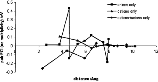
3-8 Each curve represents the pair ECI from a separate cluster expansion. The curve with red square points represents the expansion contain- ing only anion clusters. The curve with green triangles represents an expansion with only cation clusters. The curve with grey diamonds represents an expansion with clusters that each contain at least one cation and one anion. . .

3-9 The set of ECI from a cluster expansion using clusters with anion sites only contain 11 pairs and 51 triplets. The empty term is 3.907 eV. The point term is the term in the figure at the smallest cluster size. The next 11 data points connected with a line are the pair ECI from figure 3-8. The remaining 51 data points are triplets. . . .

3-10 The set ECI of a cluster expansion using clusters with cation sites only contain 5 pairs and 15 triplets. The empty term is 0.0980 eV. The ECI from empty and point clusters are labelled as in figure 3-9. . . .

3-11 The set of ECI for a cluster expansion using clusters with anion sites only contain 10 pairs and 58 triplets. The empty term is 0.0851 eV. The ECI from empty and point clusters are labelled as in figure 3-9. .

3-12 The DFT energies for 23 33

%

Yconfigurations, 60 50 % Y configura- tions, and 49 57

%

Y configurations. . . .

3-13 The anion pair terms dominate the cluster expansion of the 33

%

Y

configurations. The empty term is -2.491 eV. Circles denote pair ECI, triangles denote triplet ECI, and squares denote quadruplet ECI. In the labels for triplets and quadruplets, the not at ion 'c-c-a' indicates a cat ion-cat ion-anion triplet, for example. . .

3-14 The pair terms of the cluster expansion at 50 % Y includes all anion- anion pairs and one cation-anion cluster. The empty term is -2.530 eV . . .

3-15 The pair terms of the cluster expansion at 57

%

Y includes three anion- anion pairs, one cation-anion pair, and one cation-cation pair. The anion-anion 3nn pair does not contain a cation intermediate between the anions. The empty term is -1.844 eV.

. . .

59

4-1 The structures used in the coordination and relaxation analysis in sec- tion 4.2 are at compositions 22, 33, 44, 50, 67, and 75

%

YOl.s. The line denotes the DFT convex hull.

A

plus mark is the energy of one unique structure, and X marks denote the energies of the ground states for reference.

. . .

68

4 2 Each point represents one 75

%

YOls structure. The 0-2Y-2Zr cluster is less likely to occur in the low energy structures.

. . .

71

4-3 The three curves indicate the slope of the probability deviation from random for a particular cluster occupation versus formation energy. The clusters are the three occupation types of a cation tetrahedron around an oxygen. Plus marks on a solid line indicate the tetrahedron with three ytrrium and one zirconium,

X

marks on a dashed line in- dicate the tetrahedron with two yttrium and two zirconium, and an asterisk on a dotted line indicates a tetrahedron with one yttrium and three zirconium.

. . .

72

4-4 An analogous plot to figure 4-3 for the occupation of the cation tetra- hedron around a vacancy.

. . .

72

4-5 Each point represents one 50 % Y01.5 structure. The average relax- ation around the oxygen in a structure decreases toward higher energy structures..

. . .

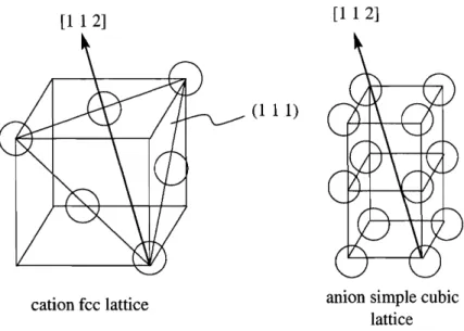
74 4-6 Each point represents the slope of the average cation relaxation around

4-7 Yttrium and vacancies align in the [l 1 21 directions in (1 1 1) planes in the ground states. The figure on the left shows the cations on an fcc lattice, and the figure on the right shows the [l 1 21 direction on a

. . .

simple cubic lattice.

4-8 Large red ions are oxygen and small orange spheres represent oxygen vacancies. The middle sized ions represent cations. The dark grey Zr and light green Y cations are on face centered cubic positions. The figure shows the unrelaxed cubic positions. Figure (a) shows a supercell of the ground state at 25

%

Y01.5. The horizontal planes are (1 1 1)) and the viewing direction in to the page is [l 1 21. Figure (b) shows a supercell of the primitive cell with some cubic cell vectors included. . 4-9 The key is the same as in figure 4-8. This structure is the ground state at 29

%

Y01.5. . . .

4-10 The key is the same as in figure 4-8. This structure is the ground state at 33 %Y01.5.

. . .

4-11 The key is the same as in figure 4-8. This structure is the ground state

at 5 7 % Y o 1 . 5 . . . .

4-12 Figure (a) is the density of states for cubic ZrOz. Figures (b) and (c) show the density of states for the ground states at 25 and 29

%

YOlo5, respectively. The thick grey dashed lines are Zr d states, and the thin green lines are Y d states. The thin dashed-dotted red lines are 0 p states. The units of energy are eV. . . .

4-13 Figures (a), (b), and (c) are the density of states for the ground states at 33, 57, and 100 % YOlq5, respectively. The units of energy are eV. 4-14 In canonical Monte Carlo cooling of the 33

%

Y ground state, the peak

in heat capacity differs depending on the type of site exchange. For nearest neighbor site exchanging on both cat ion and anion sublat t ices, the peak is at 1500 K. With a fixed cation sublattice and only nearest neighbor anion site exchanges, the peak is at 1750 K. . . .

4-15 The plot contains one data point for each cluster in the cluster ex- pansion. The ordinate value for each point is the difference between the correlations in the cooled 500

K

Monte Carlo state and the start- ing 3500

K

state for a canonical nearest neighbor exchange simulation. The points are sorted by decreasing magnitude. The labels of the first thirteen clusters are in the order of decreasing absolute magnitude and correspond to the cluster list in appendix

B.

. . .

92

4-16 The lowest excitation energies for the ground state structures are 0.695,

. . .

1.038, 0.984, and 1.568 eV, in order of increasing

Y

composition. 93

5-1 The plot of the electron localization function in the (1 1 1) cation plane of the ground state structure with 33

%

Y

shows rings around cation positions and circles of red where charge localizes on oxygen sites from neighboring (1 1 1) planes. Red indicates the fullest degree of localization and green indicates delocalized charge. The degree of localization for Zr and

Y

is similar, with the Zr localization extending

. . .

closer to the neighboring oxygen than the

Y

localization. 97

5-2 The cation relaxation curve gives the difference in energy between the ground state with cation sites allowed to relax and anion sites fixed and the ground state with anion and cation sites relaxed. The anion relaxation curve is the analogous difference in energy but with the first structure being the ground state with anion sites allowed to relax and cation sites fixed.

. . .

99

5-3 Each plot contains

V i

for each cation in the unit cell in the unrelaxed, fully relaxed, anion relaxed, and cation relaxed structures for ground

. . .

states with 25 % (a), 29 % (b), 33 % (c), and 57 % (d) Y. 102

5-4 The plot shows formation energies of structures in the zirconia-scandia system with respect to cubic ZrOz and C-type ScO1.j. The structures with 25 and 33

%

Sc are the YSZ ground state configurations with Sc replacing Y. Points labelled Sc-delta and Sc-gamma show the energies of the reported stable phases at their compositions. Points labelled YSZ-29% and YSZ-delta show the energies of the YSZ ground state configurations with Sc in Y sites. . . . 107 C-1 The probability deviation from random for a vacancy coordinated by

one yttrium and three zirconium. . . . 120 C-2 The probability deviation from random for a vacancy coordinated by

two yttrium and two zirconium. . . . 121 C-3 The probability deviation from random for a vacancy coordinated by

three yttrium and one zirconium. . . . 122 C-4 The probability deviation from random for an oxygen coordinated by

one yttrium and three zirconium.

. . .

123 C-5 The probability deviation from random for an oxygen coordinated by

two yttrium and two zirconium. . . . 124 C-6 The probability deviation from random for an oxygen coordinated by

three yttrium and one zirconium. . . . 125 C-7 The average relaxation of cations around oxygen for the six composi-

List

of

Tables

4.1 Table (a) contains the fully relaxed unit cell and atom positions of the 25

%

ground state structure. Table (b) contains the fully relaxed unit cell and atom positions of the 29

%

ground state structure. . . 76 4.2 Table (a) contains the fully relaxed unit cell and atom positions of the

33

%

ground state structure. Table (b) contains the fully relaxed unit cell and atom positions of the 57

%

b-ground state structure. . . 77 4.3 The table lists the average relaxed metal-oxygen bond lengths for each

Zr and Y in a ground state structure. . . 80

5.1 The table lists the bond valence parameters for yttrium, scandium,

. . .

and zirconium with oxygen [I]. 100

5.2 The radii of the transition metals vary by their coordination in a com-

. . .

pound[2]. 105

B. 1 The table lists the pair clusters of the cv score minimizing cluster ex- pansion with their labels (in parenthesis) and the ECI with multiplicity

. . .

included. 116

B.2 The table lists the triplets of the cv score minimizing cluster expansion with their labels (in parenthesis) and the ECI with multiplicity included. 117

. . . B . 3 Table B. 3 is a continuation of table B. 2. 11 8

Chapter

1

Introduction

Yttria-stabilized zirconia (YSZ) is an important material for its use as an oxygen ion conductor. An understanding of the interaction among ionic species in the Zr02-Y203 system would be useful for optimizing the material's conductivity. The computational studies in this dissertation show that the Zr02-Y203 system exhibits stable, ordered ground state structures and that driving forces contributing t o phase stability depend on composition: oxygen relaxation contributes t o stability at low compositions of yttria, and the arrangement of cations contributes t o stability at high compositions of yttria.

Conductivity

Pure monoclinic zirconia exhibits negligible oxygen ion conductivity, but with the ad- dition of yttria, the system takes a cubic fluorite structure. The oxygen conductivity increases to reach a maximum of 10-I (ohm

.

cm)-' at 1000 K with 15-18

%

(8-10

%

Y203) [3, 41. With the addition of 20

%

more Y01.5 doping, the conductiv- ity decreases by an order of magnitude. Numerous computer modelling studies have attempted to explain the mechanism of diffusion in doped zirconias and the reason for a peak and subsequent decrease in conductivity with more doping v[5, 6, 7, 8, 91. For each Y 2 0 3 molecule added to Zr02, one vacancy forms to maintain charge balance in the material. As yttria is added to zirconia, the concentration of vacan-

cies, and hence available oxygen hopping sites, increases. The conductivity, however, decreases. One possible explanat ion involves the oxygen diffusion pathway. Oxygen ions diffuse along pathways between two cation sites, and studies suggest a path- way between two large yttrium ions is unfavorable [5, 81. As the composition of the material increases above 15-18

%

Y01.5, the Y-Y unfavorable pathways inhibit conductivity. Another possible explanation for the decrease in conductivity is the ordering of oxygen vacancies. A driving force for order would resist oxygen hopping in to ordered vacant sites. Evidence exists for short range order of vacancies [lo].

1.2

Structure

and phases

Pure zirconia and yttria have fluorite based structures. The cubic fluorite structure has cations on face centered cubic positions and anions in the tetrahedral interstices of the fcc lattice (figure 1-1). Another representation of the structure is to consider anions in a simple cubic array with a cation inside every other oxygen cube. Each cation site has eight nearest neighbor anion sites, and each anion site has four nearest neighbor cation sites.

Pure ZrOz is cubic fluorite at high temperatures. From the cubic fluorite structure, zirconia transforms to a tetragonal structure at 2350 "C. The tetragonal structure is a result of a distortion of the oxygen sublattice along the

Xc

mode of vibration, which causes [0 0 11 rows of oxygen to be offset alternately up or down with respect to the fcc cation lattice (1 11. Continued cooling yields the monoclinic ground state structure at 1100 "C. The monoclinic structure is a further distortion of the cubic fluorite structure such that each zirconium has seven oxygen at the nearest neighbor positions.

The structure of pure yttria is the C-type lanthanide structure, where the letter C

is an abbreviation for cubic. The structure is based on cubic fluorite, but one-fourth of the anion sites are vacant. The conventional unit cell is body centered cubic with 80 atoms. One way to visualize the vacancy arrangement in C-type structure is that the vacancies align along four nonintersecting (1 1 1) chains so that every yttrium has

Figure 1-1: The cubic fluorite structure has cations (Y, Zr) on fcc sites and oxygen and vacancies in tetrahedral interstices. The light green cation is yttrium, which is 0.2

A

larger in radius than zirconium in grey.

six oxygen nearest neighbors [12]. The structure may also be visualized as a set of

64 simple anion cubes (a 4 x 4 ~ 4 array) with yttrium filling half of the cubes. Three- fourths of the cubes have two vacancies at face diagonal positions and one-fourth have

two vacancies at cube diagonal positions.

When yttria is added to zirconia, the monoclinic zirconia transforms to tetragonal and then cubic fluorite. The term yttria-stabilized zirconia refers to the cubic fluorite

phase of zirconia, which is stabilized over the monoclinic structure as a consequence of

incorporating yttria. At compositions between pure Zr02 and pure Y203, experiments

have verified the existence of one ordered structure with stoichiometry Y4Zr3012

[13, 141. In materials with low yttria (less than 50

%

YOla5) concentration, ongoing

research investigates the driving forces for short range order of cations and anions.

Some studies suggest that phase separation between pure yttria and another ordered compound may occur at compositions between Y4Zr3012 and pure yttria [15, 16, 17, 181, but other investigations do not confirm those findings[l9, 20, 21, 221.

The compositions of the materials discussed in this dissertation are written with

tween

%

YOlms and

%

Y203:

1.3

Investigations of order and phase stability

This work investigates the ordering and phase stability across the ZrOzY203 compo- sition range. The calculations show the presence of stable, ordered ground states on the cubic fluorite lattice and composit ion-dependent driving forces for phase st ability. Chapters 2 and 3 describe the cluster expansion technique and its application to the yttria stabilized zirconia system. Chapter 2 is a practical guide for implementing a cluster expansion, and chapter 3 presents the cluster expansion of YSZ. The cluster expansion has led to the identification of previously unknown ordered ground states. An evaluation of the ground state structures in chapter 4 shows the relationships among their atomic ordering and electronic structure.

Chapter 4 also offers insight in to the driving forces for stability in YSZ. Three parts of the chapter describe the complex nature of ordering: a survey of the lit- erature on ordering and phase stability, an analysis of how the cation coordination and relaxation around oxygen varies across the composition range, and Monte Carlo calculations of the configurational changes of one ground state with temperature. Chapter 5 parses some factors that are important for understanding phase stability and quantifies the impact of oxygen relaxation, vacancy ordering, and cation size on the stability of the ground states.

Chapter 2

Cluster expansion implement at ion

2.1 Developing a cluster expansion

A

cluster expansion is a method to model the energetics of a material using insight from both physics and statistics.

A

cluster expansion in theory provides an exactly converging expression of the energy in terms of configuration variables; in practice, complex systems require the cluster expansion to be optimized for a specific purpose rather than providing the exact energy convergence. This chapter offers a guide for defining the purpose a cluster expansion, met hods for choosing structures and clusters to be included in the fit, and metrics for analyzing the results.

Section 2.1 defines the cluster expansion and suggests common purposes. Section 2.2 describes metrics like rms error and cross validation score to quantify how well the fit reproduces the original data, and section 2.3 details factors for consideration or methods that can be employed to choose the structures and clusters used for implementation. Comparing the implement ation and results with the purpose of the

fit determines whet her the cluster expansion is complete.

2.1.1 Cluster expansion background

The main achievement of the cluster expansion formalism is to rigorously quantify the configurational disorder of a system by an orthogonal expansion of basis functions.

This is accomplished by parameterizing the energy in terms of the atom types placed on lattice sites. Given a structure with two components, an Ising lattice provides a model for the lattice sites of the solid. To compare different configurations of atoms within a single material system, all structures must map on to the same Ising lattice type.

A

spin variable, ai, of +1 or -1 denotes what type of atom is on each site i.

Rather than specifying the type of atom on each lattice site within a particular structure, a complete set of orthonormal basis functions can also specify the configu- ration of a structure. The basis functions called cluster functions are polynomials of the discrete variables ai.

A

cluster function, a, is the product of the spin variables at one or more sites. The cluster of just one a site is called a point cluster.

A

cluster of two sites is called a pair.

A

cluster of three sites is a triplet. To simplify the cluster expansion, one can group together clusters that are symmetrically equivalent. If a cluster can be mapped on to one another cluster by operation of one or more symmetry elements of the parent structure, the two clusters belong in the same group called an orbit

R,.

The average of the spin variable products over all the clusters in the orbit is given by

-l

where N is the number of clusters ,6' in the orbit. (&(a')) are called the correlation functions.

Using the cluster functions as the basis for the expansion of the energy, the pa- rameterization of the energy takes the form

where ma is the multiplicity of cluster a and Np is the number of Bravais lattice points. The coefficients of the expansion V, are the effective cluster interactions

(ECI). The cluster expansion is an exact expansion of the energy. Truncating the expansion introduces error. In matrix notation, the cluster expansion becomes a

mathematical fit :

Ern = X m x n V n

where Em is a vector of m structural energies, X,,, is a matrix of the n correlations for each m structures, and V, are the n ECI to be fitted. An excellent summary of the cluster expansion formalism is available in A. van der Ven's thesis [23] and a thorough review is in a book chapter by D. de Fontaine [24].

2.1.2

Purpose of the cluster expansion

The task of someone implementing a cluster expansion is how to choose clusters a

and structures (and hence their energies E) for equation 2.2 to create a useful model. The primary result of the cluster expansion is the set of ECI. Since the expansion is exact, the theoretical values of the ECI depend on the overall energetics of the system, but in practice, the truncation of the expansion and the particular cluster functions and structural energies chosen for the fit will determine the specific ECI values obtained. By defining one or more purposes for the cluster expansion, choices during the development of the cluster expansion will guide one to obtain useful results. A cluster expansion has many potential purposes:

to predict and identify the ground state structures at one or more compositions to function as a Hamiltonian for Monte Carlo to model relative phase stability in a specific temperature range (for phase diagram calculations, for example) to infer local contributions to a structure's energy and hence driving forces for order /disorder

to accurately represent the energetics of structures in a particular energy range Referring to the last item in the list as an example, to go from a statement of purpose to the implementation of the cluster expansion, one must be specific and quantita- tive. What structures are 'representative' of the system? How many structures are

necessary? What cluster functions give the degrees of freedom necessary for 'represen- tative' energetics? What metric defines an accurate representation: a small difference between the calculated and fitted energies or ECI values following physically rational behavior?

To help answer quest ions like these, the following sect ions suggest quantitative measures of accuracy and suggest methods to choose structural energies and clusters for modeling a system of interest. Experience with the cluster expansion of yttria stabilized zirconia provided a foundation of thought and experience for this chapter. For details on the cluster expansion of

YSZ,

see chapter 3.

2.2

Metrics of the expansion

A

cluster expansion is a fit of structural energies to the correlation variables that describe the structures' configurations. The structures included in the fit are a subset of all possible configurations of the system. Metrics quantifying the errors of the cluster expansion help evaluate the usefulness of the resulting fitted ECI. Two sys- tematic types of error can arise in a cluster expansion: the differences between the calculated energies and fitted energies within the subset structures of the expansion and the differences in ECI between the whole set of configurations of the system and the subset of structures included in the fit. Throughout this thesis, the definition of

the calculated energy is the energy of a structure calculated with DFT, electrostatic,

potential model calculations, or other total energy methods. The fitted energy of a structure is the energy found by multiplying the fitted ECI with the correlations of the structure.

Consider the difference between the calculated and fitted energies of the structures in the fit. As more cluster functions are included in the cluster expansion, the fitted energies converge upon the calculated energies [24]. A cluster expansion in practice, however, truncates the fit to a finite number of clusters. Removal of clusters that would further converge the fit cause an error called bias in the fitted ECI. Now consider the error called variance; it is the statistical deviation around a mean value.

As the number of structures in the sample increases, the mean of the sample converges to the mean of the whole population of structures. The average deviation from the mean, however, is sensitive to the particular energies and correlations in the fit. That deviation is the variance. The four metrics below help quantify the errors in the fit.

2.2.1

Root mean squared error

The residual error of a structure's energy is the difference between the calculated energy, E,, and the fitted energy E ~ . The root mean squared (RMS) error of the fit is the average of the squared residual error of all the structures

RMS error =

N

RMS

error is the simplest estimation of goodness of fit for the set of structures in the cluster expansion. It does not measure the ability of the cluster expansion to predict the energies of structures not in the fit.

2.2.2

Cross validat ion score

The cross validation score measures the ability of the cluster expansion to predict the energy of a structure left out of the fit. In leave-one-out (n=l) cross validation (cv), one removes a single structure from the fit, uses the remaining structures to obtain ECI, and calculates the residual error on the energy of the removed structure. The procedure is done successively for every structure in the fit. The average root mean squared error of all the residual errors is the cv score.

2.2.3

ECI

error

In the least squares fit, a standard error of the fitted ECI arises when there are more structural energies than clusters included in the fit. The fitted ECI minimize the difference between the fitted energies and the calculated energies for all the structures.

The standard error of the ECI, s~ is

s2- is the estimated variance of the energy residuals

Ei

2 2

s-. =

cL1

( E ,

-

$)

Ei n - k

where n is the number of energies in the fit and k is the number of ECI. The cii are

the variances of the ECI. A derivation of the ECI variance is in Appendix

A,

and the covariance subsection of section 2.3.1 discusses this further.

The appendix explains that each row of the matrix

X

contains the correlations for the clusters in one structure, and cii are the diagonal elements of the matrix

(XTX)-I

.

If the correlations of the structures have high covariance with each other, then the

XTX

matrix will approach singularity. As the matrix approaches singularity, the values of cii will increase indicating that the ECI estimates may be imprecise, and the fitted ECI will deviate from the theoretical ECI.

2.2.4

Cluster expanded energy

of

trial structures

One useful capacity of a cluster expansion is the ability to quickly obtain estimated energies for uncalculated structures. Given the ECI from a set of fitted structures, one can calculate an approximate energy using the fitted ECI and the correlations for the structure of interest that was not included in the cluster expansion. If the purpose of the cluster expansion includes searching for ground state configurations, knowing approximate energies of unfitted configurations accelerates the search process. High energy structures may be discounted if they are not considered candidate ground states. The cv score offers a predictive measure of the fit using the energies and correlations already in the cluster expansion. Calculating the energy of a set of trial, unfitted structures with the ECI of a fitted sample set offers a predictive measure of the energies in the correlation space not in the fit. The set of trial structures

may be orders of magnitude larger than the set of fitted structures. If some trial structures have energies below the convex ground state hull, these trial structures may potentially be ground state configurations (figure 2-1).

potential

I

ground states

I

composition (x)

Figure 2-1: Calculating energies of trial structures using the

ECI

of the fitted config- urations can be useful to identify potentially stable structures. Circles denote fitted energies of structures in the cluster expansion. Triangles represent estimated energies of trial structures calculated from

ECI.

Using DFT or other total energy method, one can calculate the energies of the potential ground state structures (triangles) to determine if one is a true ground state.

2.3

Factors for implement at ion

Two approaches exist for determining what clusters and structures to include in the cluster expansion. One approach involves choosing clusters and structures that have particular physical or statistical characteristics with the desire that they will adequately model the system. The other approach involves selecting clusters and structures regardless of their individual properties until the final fit has particular statistical characteristics. The two approaches ideally converge on the same solution,

although praxis shows this convergence is not guaranteed.

2.3.1

Cluster choice

In the practice of putting together a cluster expansion, the number of distinct clusters possible to enumerate on a lattice is 2 N , where N is the number of lattice sites. The number of structures for which it is possible to calculate energies is limited by computational resources. Since fitting a larger number of clusters to a fewer number of energies creates an undetermined fit, truncating the cluster expansion to include a subset of the possible cluster functions gives a more rigorous set of ECI. The decision to include a particular cluster in the fit depends on whether it has a desirable physical arrangement of the points in the cluster or whether the cluster's correlations have a desirable affect on the quantitative metrics of the fit. All of the methods described below, except the last one, select clusters based on their physical or statistical properties. The last method follows an outcome approach that chooses clusters arbitrarily to minimize the cross validation score of the final fit.

Including subclusters

A common property of convergent cluster expansions is that every subcluster of each included cluster is in the expansion. The subclusters of a pair are the pair clusters that are smaller in range. Figure 2-2 gives an example.

Covariance between clusters

According to standard statistical fitting practice, when variables are highly covariant

,

the coefficients of those variables do not represent the independent contribution of each variable to the observation. In a cluster expansion, the observation is the cal- culated energy of the structure. The covariance between two clusters is the degree to which the variance of the correlations of one cluster moves with the same sign, opposite sign, or independently of the variance of the correlations of another cluster

triplet

neighbor

Figure 2-2: The square cluster in (a) has three subclusters: the pair subclusters in (b) and the triplet in (c).

xi and X j are two sets of correlations, and pi and p j are the sample means of xi

and Xj. When C O V ( X ~ , X ~ )

>

0, then X j tends t o increase when xi increases. When

C O V ( X ~ , X ~ )

<

0, then x j tends to decrease when xi increases. When C O V ( X ~ , X ~ ) = 0, the correlations are independent. In statistical fitting, independent variables provide the most explanatory power. A cluster expansion, however, is not a pure statistical fit of data. As Sanchez shows, a convergent solution t o fitting cluster functions t o the energies is possible [25]. In the whole configuration space, the correlations of the clusters create an orthogonal set of vectors. When considering a finite set of correlations for the structures in a cluster expansion, however, subclusters can be highly covariant with their parent cluster. Since the subclusters can, in practice, add covariance to the matrix of correlations, a physical cluster expansion and a statistical fit may be at odds with each other. Note that in statistical literature, the covariance normalized by the product oigj is called the correlation between xi and X j , where

oi and oj are the variances of xi and xj. The statistical correlation between xi and x j is different from the cluster expansion correlation defined earlier in equation 2.1.

The term correlation in this thesis always refers t o the cluster expansion correlation unless specifically noted otherwise.

Analytical terms

In the standard construction of the cluster expansion, the formation energies of a set of configurations are fit to the correlations of clusters defined by geometrical point arrangements. Subtracting off a known, analytical portion of the energy from the formation energy may improve convergence by removing a degree of freedom from the energies to be fit by the correlations. The electrostatic energy between point charges on a periodic lattice, for example, has been worked out in an Ewald sum [26]. The real space Ewald term

Er

is

Subtracting off

Er

from the energy is analogous to adding a term to the cluster expansion

where the last term of equation 2.10 is a weighted sum of the pair correlations.

rr

are the pair correlations,

a

is a damping parameter, and ri is the distance between two points in the ith pair cluster.

Another example of accounting for portions of the energy analytically is in the mixed space cluster expansion (MSCE) [27, 28, 291. MSCE uses the traditional cor- relations and ECI for all clusters except the pair terms. Employing earlier work on reciprocal-space expansions [30], it uses the Fourier transforms of the ECI and correlations for the pair terms.

The constituent strain (cs) energy,

AE::(X,~),

is the energy necessary to maintain coherency at an interface between regions of each pure component. It depends on the orientation

k

of the interface.

Minimizing cross validation score

The previous approaches in section 2.3.1 use a building approach of choosing clusters, whereby clusters are f i s t chosen by their physical or geometrical significance without knowing the final impact on the metrics of the expansion. Outcome approachs are possible that iteratively choose clusters in an arbitrary manner to optimize an aspect or metric of the final cluster expansion. The statistical literature explains the use of leave-one-out cross validation (cv)

,

Mallow's C, [3 11 and Akaike's Information Criterion (AIC), as well as describing the bootstrap and jackknife methods [32], for choosing variables/clusters. These five methods are asymptotically equivalent [33,34].

Li [35] and Shao [36] discuss the use of cross validation methods to choose variables for the best predictive model of a system. Li proves, and van de Walle [37] summa- rizes, that if the number of observations (structural energies) in the fit increases as the number of variables (clusters) added to the model increases, minimizing the cross val- idation score finds the the optimal, most predictive model. Van de Walle explains this result using the decomposition of the expected squared error of the cluster expanded energy. A paraphrase of his explanation gives the essential details [37]:

If yi is the energy of a structure with correlation vector

Xi.

Each correlation vector Xi contains k elements, one for the average value of each cluster in structure i.

fii

is the predicted energy of structure i from the cluster expansion of N total structures. A decomposition of the expected squared error gives

and the last term is the covariance term. In a least squares fit of the

N

structural energies, the covariance term will be positive and increase as

$

increases. The ex- pected error is therefore sensitive to the number of clusters and structures in the fit, regardless of their individual characteristics. Consider if iji is replaced by which is the energy of structure

i

predicted fiom a cluster expansion of all structural energies except the energy of i (hence N-1 structures in total). Now the covariance term goes to zero, and the change in the variance term goes to zero as N increases. This provides more accurate predictive power. The CV score is the sample average of (iji-m - ~ i ) .

The remaining step is to choose a procedure for adding variables most efficiently to the model. The literature lists several methods: forward selection, backward elimina- tion, stepwise, branch-and-bound, and simulated annealing [32]. Of greatest interest is simulated annealing because of its use as a search method in global minimization problems. Based on Monte Carlo simulations, adding or subtracting a cluster to the cluster expansion will increase or decrease the cv score. When the cv score de- creases, the cluster is accepted. When the cv score increases, the cluster is accepted if the probability of it occuring is greater than a randomly chosen number. The au- thor acknowledges Tim Mueller for proposing the Monte Carlo approach of choosing structures.

2.3.2

Structure choice

The calculated energies of structures are the computational observations that lead us to make conclusions about a system's configurational behavior. In standard statis- tical practice, the sample of a population is a random selection of data points from a whole population. In the cluster expansion, the fit of ECI is not a pure statistical process, and randomly selecting structures may not be the best approach to model a system's configuration. Since the ECI are a convergent series to the exact solution, random selection will invariably lead to the selection of large supercell structures. Ex- isting computers cannot calculate large supercell structures (lo3-lo4 atoms or larger, depending on energy method) in an acceptable amount of time; therefore, calculating

large structures may not be feasible modelling option. Depending also on the purpose of the cluster expansion, all structures of a given system may not be of interest. In- herent in the selection of structures is the decision about whether to choose structures that either widely sample or narrowly sample the available correlation space.

The first four methods below choose structures for the fit based on the struc- tures' physical characteristics. The sections on sensitivities and orthogonality use an approach that chooses structures based on their correlations t o directly create a clus- ter expansion modelling a particular range of correlation space. The last section on weighting describes an approach to add elements t o the energy vector and correlation matrix to optimize the cluster expanded convex hull outcome.

Structures by energy

Structures may be sorted by their formation energy. Structures with a high formation energy are unlikely to stabilize experimentally, while structures with a low formation energy are more likely t o be stable or metastable phases. Low energy structures model the configurational landscape near the convex hull. One approach in a successful cluster expansion was to include only low energy structures near the convex hull in the fit [38].

Supercell size

The structures that model a material system come from configurations of atoms on various supercells of the primitive lattice unit cell. Small supercell sized structures have simple ion geometries due to the few number of sites for repetition, and larger supercell structures have more complicated geometries. Small sized structures may model some material systems well, while other systems may require large structures. Including complicated geometries adds additional complexity for the cluster expansion t o model.

Along with the geometrical attributes of supercell sizes is the effect of choosing different compositions. The supercell size limits the number of compositions that the cluster expansion models. The number of compositions that can be modelled may be

important if many structures at small composition increments are stable (a Devil's staircase) [39].

Experimental information

Experiments on the system of interest can yield clues about what the expected or- dering and ground state structures are and guide the selection to a group of possible ordered structures [40].

Cluster expanded predicted structures

Estimating energies of uncalculated trial structures is possible using the coefficients of the cluster expansion. When the cluster expanded energy is lower than the hull of the current fit, the structure may have a true, calculated energy that is also below the hull. To predict the ground state structures of the system, that potential structure needs t o be calculated to verify its energy. With enough iterations, this method can find previously unidentified ground state structures, if they exist. Section 2.2.4 also discusses the approach.

Sensitivities

One way to quantify the range of correlation space sampled by the structures' corre lations is t o use singular value decomposition (SVD). The SVD of the

X

matrix of correlations decomposes it into

X = U S V ~ (2.15)

where the columns of U are an orthonormal basis of the columns of X , the rows of

vT

are an orthonormal basis of the rows of X, and the elements of the diagonal matrix S

are the singular values [41]. The singular values indicate how the correlations sample the available correlation space. If the singular values are nearly equal, the correlations sample space evenly. If the singular values contain some very large and some very small values, the correlations for those clusters narrowly sample and widely sample correlation space.

Notice that one method t o solve equation 2.15 is with

where by diagonalizing XTX-' (the covariance matrix) gives S and V. The semi-

tivities are the diagonal elements of the (XTX)-' matrix, as shown in equation A.3.

The sensitivities relate how much the correlations vary with each other and hence are directly related t o the singular values. A small value of the sensitivity for a cluster signifies that the correlations vary greatly with each other and the correlation space is not widely sampled. The author acknowledges Chris Fischer for proposing the sensitivity approach of choosing structures.

Orthogonalizing configuration space

If the widest possible correlation space is desired, one approach is t o include structures that are most orthogonal to the current space of structures. SVD is one technique for determining the structure that is most orthogonal t o the current space of correlations [42]. The singular value with the smallest value corresponds t o vector Go of V that is most orthogonal to the correlation space. Including structures with correlations that are similar to Go will expand the region of correlation space in the fit. One method for identifying those structures is to compare

6

to a trial database of cor- relations of known structures. The author acknowledges Chris Fischer for proposing the orthogonalization approach of choosing structures.

Weighting

The previous methods listed in this section describe how t o choose structures based on the properties of the correlations of the structure. One technique that changes the fit of ECI is the weighting of particular attributes. Increasing weight on an attribute causes its energy to be more or less accurately reproduced by the fit. Weighting is possible on three kinds of attributes: an individual structure's energy, convex hull energies, and the energy difference between a particular structure's energy and

the convex hull energy at its composition. The method to mathematically include weighting into the fit depends on the type of weighting. To weigh an individual structure i, multiply each element m in the row of correlations,

oL,

for the structure and the element of the energy vector for the structure by a constant factor,

wi

.

To weigh the convex hull, an additional row of correlations for the correlation matrix and an energy element for the energy vector are necessary. One correlation row and one energy element are added for each ground state structure (not including the end point structures). Referring to figure 2-3, the energy element for the ground state structure

B

is

and the element of the row of correlations for

B

are

To weigh the energy difference,

Ek,

between the energy of a structure D and the energy of the hull, an additional energy element and correlation vector are necessary:

and similarly

The author acknowledges Anton van der Ven for the weighting schemes. 42

0 1 composition (x)

Figure 2-3: Adding elements to the energy vector and correlation matrix will empha- size attributes of the cluster expansion. One attribute, for example, is the energy difference

Ek

between a structure and the hull.

2.3.3 Mathematical fitting

Several mathematical techniques exist to determine the relationship between the clus- ters and the energies. Least squares minimization, linear programming, principal components, partial least squares, and Ridge regression are all available techniques. Ridge regression is also known as the weight decay method in neural networks. In cluster expansions, the least squares method and linear programming are the most common methods to determine ECI. Least squares minimization seeks to minimize the root mean squared error of the energies. Linear programming seeks to find a space of available solutions and choose the solution which optimizes an objective function of those variables [44]. The techniques may give similar but distinct results and are both viable options for determining ECI.

Chapter

3

Cluster expansion

of

Zr02-YOls5

using nrst principles energies

3.1

Expansion on coupled sublat

t

ices

The cluster expansion of Zr

Oz-YO

is different from a traditional binary cluster expansion because configurational disorder exists on two types of sites: the cation fcc sites with Y and Zr and the anion simple cubic sites with oxygen and vacancies. For every two yttrium on the cation sites, one vacancy is necessary on an anion site to maintain charge balance. The cations and anions do not mix between their respective fcc and simple cubic sublattices, but the equilibrium configurations on each sublattice may depend on the other. To model the possible dependence between sublattices, the cluster expansion couples the sublat t ice configurations by including clusters that contain at least one cation site and one anion site. The model for YSZ only considers structures on a cubic lattices; monoclinic and tetragonal phases of zirconia are not considered.

3.2 Energies from first principles

Configurations of the cluster expansion of YSZ came from a variety of sources. C. Wolverton and A. Bogicevic at the Ford Motor Company chose the first 90 structures

and calculated the total energy of each. Their investigations of YSZ used configura- tions a t 25, 29, 33, 50, and 57

%

Y01.5

[40, 45, 461. Using lattice algebra techniques, they determined unique cation configurations on the face-centered cubic sublattice and then decorated the simple cubic anion sublat tice [40].

Selection of structures to calculate and add to the initial set for this investigation followed the methods in section 2.3.2. A useful source of structures was a database of all 81827 configurations that are possible in supercells consisting of 9 primitive fcc unit cells or smaller on the fluorite lattice. Each primitive unit cell has 1 cation and 2 anion sites.

The total energy of each structure is obtained with the VASP implementation of Density Functional Theory (DFT) in the Generalized Gradient Approximation (GGA) with the PW91 exchange-correlation functional. The calculations use ultrasoft pseu- dopot entials. Beginning with configurations of ions in ideal cubic fluor it e positions, the calculation allows ion positions and volumes to relax during energy minimization with a 2 x 2 ~ 2 k-point mesh. Starting from the 2 x 2 ~ 2 k-point mesh relaxed configura- tion, a calculation of the total energy using a 4 x 4 ~ 4 k-point mesh gives the final total energy. Calculations of some structures with a 6 x 6 ~ 6 k-point mesh ensure that the 4 x 4 ~ 4 k-point mesh is adequate for k-point convergence. The fit does not include any structure having ions that relaxed more than half of the distance from its original site to its first nearest neighbor.

The final YSZ cluster expansion contains the energies of 447 structures. Figure 3-1 shows the DFT formation energies of the structures. The ground states of the system are cubic Zr02, C-type Y203, and structures with 25, 29, 33, and 57 % YOle5. The structures with 25, 29, and 33

%

YOlm5 have not been previously identified on the cubic lattice as stable structures on the convex hull. Descriptions of the ground state structures are in chapter 4.

Y composition

Figure 3-1: The

DFT

energies of configurations in the cluster expansion are a t 15 compositions: 0, 22, 25, 29, 33, 44, 50, 57, 67, 73, 75, 80, 86, 89, 100

%

Yo1.5.

3.3

Cross validation score minimization

3.3.1

Clusters

To select clusters, a Monte Carlo-like approach was used to chose clusters that mini- mize the cross validation score [47]. Minimizing the cv score theoretically converges the cluster expansion on the optimal fit of the correlations to the energies (see sec- tion 2.3.1). To choose clusters for the expansion, the searching algorithm selects a cluster at random from a set of enumerated clusters. If including the correlations of that cluster in the expansion decreases the cv score, the algorithm includes the cluster. If the cluster increases the cv score, the algorithm accepts the cluster when the following condition holds:

eup

( k )

>

random number

~ B T