HAL Id: hal-02359540
https://hal.archives-ouvertes.fr/hal-02359540
Submitted on 12 Nov 2019HAL is a multi-disciplinary open access archive for the deposit and dissemination of sci-entific research documents, whether they are pub-lished or not. The documents may come from teaching and research institutions in France or abroad, or from public or private research centers.
L’archive ouverte pluridisciplinaire HAL, est destinée au dépôt et à la diffusion de documents scientifiques de niveau recherche, publiés ou non, émanant des établissements d’enseignement et de recherche français ou étrangers, des laboratoires publics ou privés.
Word Recognition, Competition, and Activation in a
Model of Visually Grounded Speech
William Havard, Jean-Pierre Chevrot, Laurent Besacier
To cite this version:
William Havard, Jean-Pierre Chevrot, Laurent Besacier. Word Recognition, Competition, and Activa-tion in a Model of Visually Grounded Speech. Proceedings of the 23rd Conference on ComputaActiva-tional Natural Language Learning (CoNLL), Nov 2019, Hong Kong, China. pp.339-348, �10.18653/v1/K19-1032�. �hal-02359540�
Word Recognition, Competition, and Activation
in a Model of Visually Grounded Speech
William N. Havard1,2, Jean-Pierre Chevrot2, Laurent Besacier1 1LIG, Univ. Grenoble Alpes, CNRS, Grenoble INP, 38000 Grenoble, France
2 LIDILEM, Univ. Grenoble Alpes, 38000 Grenoble, France
Abstract
In this paper, we study how word-like units are represented and activated in a recurrent neu-ral model of visually grounded speech. The model used in our experiments is trained to project an image and its spoken description in a common representation space. We show that a recurrent model trained on spoken sentences implicitly segments its input into word-like units and reliably maps them to their correct visual referents. We introduce a methodology originating from linguistics to analyse the rep-resentation learned by neural networks – the gating paradigm – and show that the correct representation of a word is only activated if the network has access to first phoneme of the tar-get word, suggesting that the network does not rely on a global acoustic pattern. Furthermore, we find out that not all speech frames (MFCC vectors in our case) play an equal role in the final encoded representation of a given word, but that some frames have a crucial effect on it. Finally, we suggest that word representation could be activated through a process of lexical competition.
1 Introduction
Neural models of Visually Grounded Speech (VGS) sparked interest in linguists and cognitive scientists as they are able to incorporate multi-ple modalities in a single network and allow the analysis of complex interactions between them. Analysing these models does not only help to un-derstand their technological limitations, but may also yield insight on the cognitive processes at work in humans (Dupoux, 2018) who learn from contextually grounded speech utterances (either visually, haptically, socially, etc.). This is with this idea in mind that one of the first computa-tional model of visually grounded word acquisi-tion was introduced byRoy and Pentland(2002). More recently,Harwath et al.(2016) andChrupała et al.(2017) were among the first to propose neural models integrating these two modalities.
WhileChrupała et al.(2017) andAlishahi et al.
(2017) focused on analysing speech representa-tions learnt by speech-image neural models from a phonological and semantic point of view, the present work focuses on lexical acquisition and the way speech utterances are segmented into lexical units by a neural model.
More precisely, we aim at understanding how word-like units are processed by a VGS architec-ture. First, we study if such models are robust to isolated word stimuli. As such networks are trained on raw speech utterances, robustness to isolated word stimuli would indicate that a seg-mentation process was implicitly carried out at training time. We also explore which factors in-fluence the most such word recognition. In a second step, to better understand how individual words are activated by the network, we adapt the gating paradigm initially introduced to study hu-man word recognition (Grosjean,1980) where our neural model is inputted with speech segments of increasing duration (word activation). Finally, as some linguistic models assume that the first phoneme of a target word activates all the words starting by the same phoneme, we investigate if such a pattern holds true for our neural model as well (word competition). As far as we know, no other study has examined patterns of word recog-nition, activation and competition in models of VGS.
This paper is organised as follows: section 2
presents related works and section 3 details our experimental material (data and model). Our con-tributions follow in section4 (word recognition), section 5 (word activation) and section 6 (word competition). Section7concludes this work.
2 Related Work
In this section we explore what is known about word recognition in humans. We then review re-cent works related to the representation of
lan-guage in VGS models. A few words are also said about modified inputs and adversarial attacks as they are related to the analysis methodology used in part of this work.
2.1 Word Recognition in Humans
Many psycholinguistic models try to account for how words are activated and recognised from flu-ent speech. The process of word recognition “requires matching the spoken input with men-tal representations associated with word candi-dates” (Dahan and Magnuson, 2006). One of the first model trying to account for how humans recognise and extract words from fluent speech is theCOHORTmodel byMarslen-Wilson and Welsh
(1978). In this model, word recognition proceeds in 3 steps: access, selection and integration. Ac-cessdenotes the process by which a set of words (a cohort) becomes activated if their onsets are con-sistent with the perceived spoken input. As soon as a word form becomes inconsistent with the spoken input, it is removed from the initial cohort (selec-tionphase). A word is deemed recognised as soon it is the last one standing in the cohort. Integration consists in checking if the word’s syntactic and se-mantic properties are consistent with the rest of the utterance. However,COHORT supposes a full match between the perceived input and the word forms and does not account for word frequency in the access phase. REVISED COHORT( Marslen-Wilson,1987) later relaxed the constraints on the cohort formation to take into account these facts. There is no active competition per se between words in theCOHORTmodel. That is, the strength of activation of a word does not depend on the value of the activation of the other words, but only on how well the internalised word form matches the perceived spoken input. TRACE (McClelland and Elman,1986) is a connectionist model of spo-ken word recognition consisting of three layers of nodes, where each layer represents a particular lin-guistic unit (feature, phoneme and word). Lay-ers are linked by exitatory connections (e.g. frica-tive feature node would activate /f/ phoneme node which would, in turn, activate words starting with this sound), and nodes within a layer are linked by inhibitory connections, thus inducing a real com-petition between activated words. Contrary to the COHORT model which does not allow words em-bedded in longer words to be activated,TRACE al-lows such activation. SHORTLIST (Norris, 1994)
is another model which builds uponCOHORTand TRACEby taking into consideration other features such as word stress.1
To sum up, models of spoken word recognition consider that a set of words matching to a certain extent the spoken input is simultaneously activated and these models involve at some point a form of competition between the set of activated words be-fore reaching the stage of recognition.
2.2 Computational Models of VGS
Roy and Pentland (2002) were among the first to propose a computational model, known as CELL, that integrates both speech and vision to study child language acquisition. However, CELL required both speech and images to be pre-processed, where canonical shapes were first extracted from images and further represented as histograms; and speech was discretised into phonemes. More recently, CNN-based VGS mod-els (Harwath et al., 2016, 2018; Kamper et al.,
2019) and RNN-based VGS models (Chrupała et al.,2017) which do not require speech to be dis-cretised into sub-units were introduced. Chrupała et al. (2017) investigated how RNN-based mod-els encode language, and showed such modmod-els tend to encode semantic information in higher ers, while form is better encoded in lower lay-ers. Alishahi et al. (2017) studied if such mod-els capture phonological information and showed that some layers do capture such information more accuratly than others. K´ad´ar et al. (2017) intro-duced omission scores to interpret the contribu-tion of individual tokens in text-based VGS mod-els. More recently, Havard et al. (2019) stud-ied the behaviour of attention in RNN-based VGS models and showed that these models tend to fo-cus on nouns and could display language-specific patterns, such as focusing on particules when prompted with Japanese. Recently,Harwath et al.
(2018) showed that CNN-based models could reli-ably map word-like units to their visual referents, andHarwath and Glass (2019) showed such net-works were sensitive to diphone transitions and that these were useful for the purpose of word recognition. However, none of the aforementioned works studied the process by which words are recognised and activated. This present work aims at bridging what is known about word activation 1For a review of spoken word recognition model, reader
can consult Dahan and Magnuson(2006) and Weber and Scharenborg(2012)
and recognition in humans and the computations at work in VGS models.
2.3 Modified Inputs and Adversarial Attacks As will be shown later, the gating method used in this article modifies the input stimulus to better un-derstand the behaviour of the neural model.
We can draw a parallel with approaches recently introduced to show the vulnerability of deep net-works to strategically modified samples (adversar-ial examples) and to detect their over-sensitivity and over-stability points. It was shown that im-perceptible perturbations can fool the neural mod-els to give false predictions. Inspired by the re-searches for images (Su et al., 2019), efforts on attacking neural networks for NLP applications emerged recently (see Zhang et al. (2019) for a survey). However, while a lot of references can be found for textual adversarial examples, fewer pa-pers addressed adversarial attacks for speech (we can however mention the work ofWu et al.(2014) addressing spoofing attacks in speaker verification and ofCarlini and Wagner(2018) attacking Deep-Speechend-to-end ASR system).
3 Experimental Settings
3.1 Model Type
Even though the methodologies developed in this work could also be applied to CNN-based VGS models, the present work will solely focus on the analysis of the representations learned by a RNN-based VGS model. Indeed, from a cognitive per-spective, RNN-based models are more realistic than CNN-based models as the speech signal – or in our case, a sequence of MFCC vectors – is se-quentially processed from left-to-right, whereas in CNN-based models the network processes multi-ple frames at the same time. This will thus al-low us to explore if RNN-based models display human-like behaviour or not.
3.2 Model Architecture
The model we use for our experiment is based on that ofChrupała et al.(2017) and later modified by
Havard et al.(2019). It is trained to solve an im-age retrieval task: given a speech query, the model should retrieve the closest matching image. The model consists of two parts: an image encoder and a speech encoder. The image encoder takes VGG-16 pre-calculated vectors as input instead of
raw images. It consists of a dense layer which re-duces the 4096 dimensional VGG-16 input vec-tor into a 512 dimensional vecvec-tor which is then L2 normalised. The speech encoder takes 13 Mel Frequency Cepstral Coefficients (MFCC) vectors instead of raw speech.2 It consists of a convo-lutional layer (64 filters of length 6 and stride 3) followed by 5 stacked unidirectional GRU layers (Cho et al.,2014), with 512 units each. Two atten-tion mechanisms (Bahdanau et al.,2015) are used: one after the 1st recurrent layer and one after the 5th recurrent layer. The final vector produced by the speech encoder corresponds to the dot product of the weighted vectors outputted by each atten-tion mechanism. The model is trained to minimise the following triplet loss function as implemented byChrupała et al.(2017):
L(u, i, α) =X
u,i
X
u0
max[0, α + d(u, i) − d(u0, i)]
+X
i0
max[0, α + d(u, i) − d(u, i0)] !
(1) The loss function encourages the network to minimise the cosine distance d between an image i and its corresponding spoken description u by a given margin α while maximising the distance be-tween mismatching image/utterance pairs. For our experiments, we set α = 0.2.
3.3 Data
The data set used for our experiments is based on MSCOCO (Lin et al.,2014). MSCOCO is a data set used to train computer vision systems, and fea-tures annotated images, each paired with 5 human written descriptions in English. MSCOCO’s im-ages where selected so that the imim-ages would con-tain instances of 80 possible object categories. We trained our model on the spoken extension intro-duced by Chrupała et al. (2017). This extension provides spoken version of the human written cap-tions. It is worth mentioning that this extended data set features synthetic speech (female voice generated using Google’s Text-To-Speech (TTS) system) and not real human speech.
212 mel frequency cepstral coefficients + log of total
frame energy, vectors extracted every 10ms on a 25ms win-dow
3.4 Model Training and Results
We trained our model for 15 epochs with Adam optimiser and an initial learning rate of 0.0002. The training set comprises 113,287 images with 5 spoken captions per image. Validation and test set comprise 5000 images each.3 Model is evaluated in term of Recall@k (R@k) and median rank r.e That is, given a spoken query, which corresponds to a full utterance, we evaluate the model’s abil-ity to rank the unique paired image in the top k images. We obtain ar of 28.e
Full results are shown in Table1. Even though our results are lower than the original implementa-tion byChrupała et al.(2017), our model still per-forms far above chance level, showing it did learn how to map an image and its spoken description.
Model R@1 R@5 R@10 er
Synth. COCO 0.056 0.182 0.284 28
Table 1: Recall at 1, 5, and 10 results and median ranker on a speech-image retrieval task (test part of our datasets with 5k images). Chrupała et al.(2017) with RHN reports median ranker = 13. Chance median rank e
r is 2500.5.
4 Word Recognition
Harwath et al. (2018) observed that CNN-based models can reliably map word-like units to their corresponding visual reference. Chrupała et al.
(2017) and more recenlty Merkx et al. (2019) showed that RNN-based utterance embeddings contain information about individual words, but did not show for what type of words this behaviour holds true and if the model had learnt to map these individual words to their visual referents. Havard et al.(2019) showed that the attention mechanism of RNN-based VGS models tends to focus on the end of words that correspond to the main concept of the target image. This suggests that such mod-els are able to isolate the target word forms from fluent speech and thus segment their inputs into sub-units. In the following experiment we test if a RNN-based VGS network can reliably map iso-lated word-like units to their visual referents and explore the factors that could influence such map-ping.
3The train/dev/test correspond to those used in (Chrupała
et al.,2017)
4.1 Isolated Word Mapping
We selected a set of 80 words corresponding to the name of 80 object categories in the MSCOCO data set.4 We expect our model to be very efficient with the selected 80 words, as these are the main ob-jects featured in MSCOCO. We generated speech signals for these 80 isolated words using Google’s TTS system and then extracted MFCC features for each of the generated words. We evaluate the ability of the model to rank images containing an object instance corresponding to the target word among the first 10 images (P@10).5 Contrary to (Chrupała et al., 2017) who uses Recall@k, we use Precision@k as there are several images that correspond to a single target word. It is to be noted that at training time, the network was only given full captions and not isolated words. Thus, if the network is able to retrieve images featuring instances of the target word, it shows that implicit segmentation was carried out at training time.
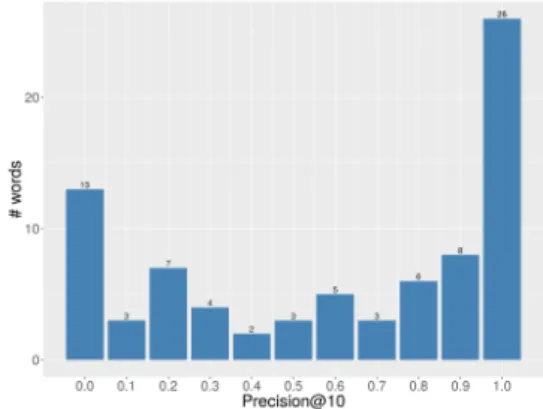
Results are shown in Figure 1. 40 words out of the 80 target words have a P@10≥ 0.8. This shows that the network is able to map isolated words to their visual referent despite never having seen them in isolation and that the network implic-itly segmented its input into sub-units.
Figure 1: Precision@10 for the 80 isolated words cor-responding to MSCOCO categories.
4.2 Factors Influencing Word Mapping We explore here the factors that could come at play in the recognition of isolated words. We explore 2 types of factors: speech related factors and im-age related factors. For the former we consider 4List available at https://github.com/
amikelive/coco-labels/blob/master/ coco-labels-2014_2017.txt
5Evaluation is performed on the test set containing 5000
Spearman’s ρ p-value Effect Images
Avg. Neighbour -0.3906 0.0003 *** Weak
Avg. Size 0.3154 0.0043 ** Weak
Avg. Freq 0.1187 0.4675 None
Text Word Freq. 0.5514 1.148e-07 *** Moderate
# Syllables -0.1211 0.2844 None
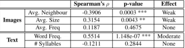
Table 2: Factors influencing word recognition perfor-mance in our model. Spearman’s ρ between Preci-sion@10 and mentioned variables as well as p-value.
word frequency (Word Freq.) and word length (# syllables). Concerning image related factors we consider object instances frequency in the images (Avg. Freq.), average number of neighbouring ob-ject instances (Avg. Neighbour), average area of each object (Avg. Size). Results are shown in Ta-ble2. We observe a weak negative correlation be-tween precison and average number of neighbour-ing objects, thus suggestneighbour-ing that objects that have a low number of neighbouring objects are better recognised by the network. It also seems that big-ger objects yield better precison than smaller ob-jects as we observe a weak positive correlation. Word frequency seems to play an important role as we observe a moderate positive correlation. How-ever, we observe no correlation between precison and the length of the target words nor with object frequency in the images. Correlation values, how-ever, remain relatively low, suggesting some other factors could also influence word recognition.
5 Word Activation
In this section we describe how individual words are activated by the network. To do so, we perform an ablation experiment (similar to that ofGrosjean
(1980) which was conducted on humans) where the neural model is inputted only with a truncated version of the 80 target words (see Section5.1). Such a method is also called gating in the litera-ture.
5.1 Gating
The gating paradigm “involves the repeated pre-sentation of a spoken stimulus (in this case, a word) such that its duration from onset is in-creased with each successive presentation”( Cot-ton and Grosjean, 1984). In our case, it means the neural model is fed with truncated version of a target word, each truncated version comprising a larger part of the target word. Truncation is either done left-to-right (model only has access to the end of the word) or right-to-left (model only has
access to the beginning of the word). Truncation is operated on the MFCC vectors computed for each individual word, meaning that MFCC vectors are iteratively removed either from the beginning of the word or the end of the word, but not from both sides at the same time. Each truncated version of the word is then fed to the speech encoder which outputs an embedding vector. As in our previous experiment, model is evaluated in terms of P@10. COHORTmodel, in its initial version ( Marslen-Wilson, 1987), stipulates that word onset plays a crucial role in word recognition whereas other models of spoken word recognition give less im-portance to word onset. This imim-portance of exact word onset matching was later revised in laterCO -HORTmodels. The aim of this experiment is to test whether word onset plays a role in word recogni-tion for the network or not. If it is the case, we ex-pect the network to fail recovering images of the target word if the word is truncated left-to-right.
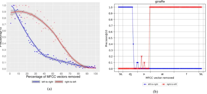
Figure 2a shows evolution of P@10 averaged over the 80 test words. As can be seen from the graph, precision evolves differently according to which part of the word was truncated. When the target words are truncated left-to-right, precision drops quickly. However, when truncated right-to-left, precision remains high before gradually drop-ping. These results show that the model is robust to truncation when it is carried out right-to-left but not when it is carried out left-to-right. Fig-ure 2b shows the evolution of P@10 for one of the target words (“giraffe”). When MFCC vectors corresponding to the first phoneme are removed (/Ã/), precision plummets from 1 to 0. How-ever, when MFCC vectors belonging to the end of the word are removed, precision plateaus at 1 until /Ç/ is reached and then plunges to 0. This shows the model successfully retrieved giraffe im-ages when only prompted with /ÃÇ/ but not when prompted with /Çæf/ even though the latter com-prises a longer part of the target word.
These results suggest that the model does not rely on a vague acoustic pattern to activate the semantic representation of a given concept, but needs to have access to the first phoneme in order to yield an appropriate representation.
5.2 Activated Pseudo-Words
Such ablation experiments also enables us to infer on what units the network relies to make its pre-dictions. Indeed, Figure 3allows us to see what
(a)
(b)
Figure 2: 2a Evolution of Precision@10 averaged over 80 test words as a function of the percentage of MFCC vector removed for each word. 2bEvolution of Precision@10 for each ablation step of the word “giraffe”, with time-aligned phonemic transcription /ÃÇæf/ at the bottom. “SIL” signals silences. For both2aand2b, blue line displays scores when ablation was carried out left-to-right, meaning that at any given part on the blue curve, model has only had access to the rightmost part of the word. (e.g. /Çæf/ without initial /Ã/). Red line displays scores when ablation was carried out right-to-left, meaning that at any given part on the red curve, model has only had access to the leftmost part of the word. (e.g. /ÃÇ/ without final /æf/ ).
Figure 3: Evolution of P@10 for each ablation step of the word “baseball bat” with time aligned phonemic transcription /beizbO:l#bæt/ at the bottom.
are the pseudo-words that were internalised by the network for the word “baseball bat”. When trun-cation is done left-to-right (blue curve), we no-tice that at the beginning precision is quite high (≈ 0.6), then reaches 0 when only /O:lbæt/ is left, but suddenly increases up to 0.9 when the only part left is /bæt/. This suggests that the network mapped both “baseball bat” as a whole and “bat” as referring to the same object. We observed the
same pattern for the word “fire hydrant” where both “fire hydrant” and “hydrant” are mapped to the same object.
However, Figure 2b shows that when only prompted with /ÃÇ/ the network manages to find pictures of giraffes. This suggests that the pseudo-words internalised by the network could be /ÃÇæf/ as a whole but might also be /ÃÇ/. We thus need to take caution when stating that the network has isolated words, as the words internalised by the network might not always match the human gold reference.
5.3 Gradual or Abrupt Activation?
Figure 2b shows that removing or adding one MFCC vector may yield large differences in the network performance. Precision decreases steeply and not steadily. This suggests that little acoustic differences yield wide differences in the final rep-resentation. Thus, in this section we analyse how representation is being constructed over time and explore if some MFCC vectors play a more impor-tant role than others in the activation of the final representation.
We progressively let the network see more and more of the MFCC vectors composing the word, iteratively feeding it with MFCC vectors starting from the beginning of the word until the network
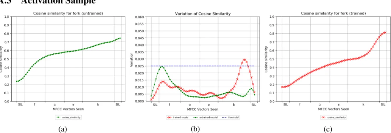
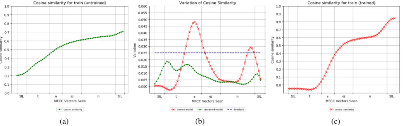
(a) (b) (c)
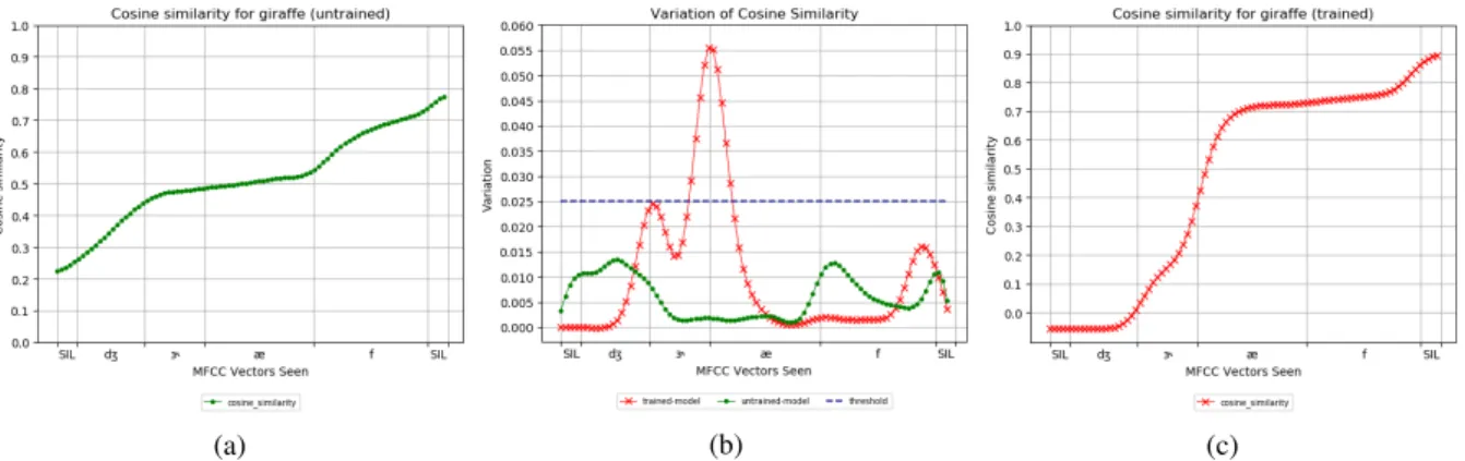
Figure 4: Figure4ashows evolution of the cosine similarity between the embeddings produced for each truncated version of the target word and the embedding for the full word using a model with randomly initialised weights. Figure4cshows the same measure with the embeddings produced by a trained model. Figure4bshows peaks indicating the inflection points of curve4a(green) and4c(red). For our experiments, we only considered inflection point to be significant if the resulting peak was higher than 0.025 (blue).
has had access to the full word. We then com-pute the cosine similarity between the embedding computed for each of the truncated version of the word and the embedding corresponding to the full word. The closer the cosine similarity is to 1, the more similar the two representations are. Thus, if each MFCC vector equally contributes to the final representation of the word, we expect cosine simi-larity to evolve linearly. However, if some MFCC vectors have a determining factor in the final rep-resentation we expect cosine similarity to evolve in steps rather than linearly. To detect steps that could occur in the evolution of cosine similarity, we approximate its derivative by computing first order difference. High steps should thus translate into peaks (e.g. Figure4b). We compute the evolu-tion of cosine similarity for the 80 target words en-coded with the best trained model (e.g. Figure4c) and also consider a baseline evolution by encod-ing the 80 target words with an untrained model (e.g. Figure 4a).6 To avoid micro-steps of yield-ing peaks and thus creatyield-ing noise, we smooth co-sine evolution curves with a gaussian filter. We consider peaks higher than 0.025 as translating a high step in the evolution of cosine similarity.
On average, they are 1.35 peaks per word for the trained model against 0.1 peak per word for our baseline condition (untrained model), showing that cosine evolution is linear in the latter but not in the former. Thus, in our baseline condition (un-trained model), each MFCC vector equally con-tributes to the final representation, whereas in our trained model some MFCC vectors are more
de-6Thus consisting only of randomly initialised weights
cisive for the final representation than others. In-deed, some MFCC vectors trigger a high step in the cosine evolution suggesting that the embed-ding suddenly gets closer to its final value. Figure
4cshows the evolution of the cosine similarity for the word “giraffe”. As it can be seen, cosine sim-ilarity does not tend linearly towards 1, but rather evolves in steps. Adding the MFCC vectors cor-responding to the transition from /Ç/ to /æ/ trig-gers a large difference in the embedding as the co-sine similarity suddenly jumps to a higher value, showing it is getting closer to its final represen-tation. However, cosine similarity plateaus once /æ/ is reached up until final silence, suggesting the final /æf/ plays little to no role in the final repre-sentation of the word.
6 Word Competition
As presented in Section 2.1, some linguistic models assume that the first phoneme of target word activates all the words starting by the same phoneme. The words that are activated but which do not correspond to the target words are called “competitors”. As the listener perceives more and more of the target word some competitors are deactivated as they do not match what is being perceived. For example, considering the follow-ing lexicon: /beIbi/ (baby), /beIzIk/ (basic), and /beIzbO:l/ (baseball), the first sound /b/ would acti-vate all three words, once /beIz/ is reached, “baby” would not be considered a competitor anymore, and once /beIzb/ is reached the only word activated would be “baseball” as it is the only word whose beginning corresponds the perceived sounds.
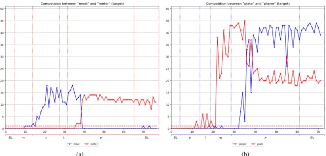
(a) (b)
Figure 5: Illustration of lexical competition between5a“meat” and “meter” (target) and5b“plate” and “player” (target). Numbers in 1st x-axis corresponds to the number of MFCC frames; 2nd x-axis corresponds to
time-aligned phonemic transcription of the target word; y-axis shows number of images for which at least one caption (out of 5) contains the target or competitor word. Vertical colour bars are projection of phoneme boundaries of the target word. Horizontal colour bars show chance score for each word (<2).
We test if the network displays such lexical competition patterns. To do so, we select a set of 29 word pairs according to the following cri-teria: i) words should at least appear 400 times or more in the captions of the training set, so that the network would have been able to learn a map-ping between this word and its referent; ii) words forming a pair should at least start with the same phoneme;7iii) words should not be synonyms and clearly refer to a different visual object (thus ex-cluding pairs such as “motorcycle” and “motor-bike”).
For each word pair, we select the longest word as target and progressively let the network see more and more of the MFCC vectors composing this word (as in Section5.3). At each time step the network produces an embedding, which we use to rank the images from the closest matching image to the least matching image.8 Then, for the 50 closest matching images, we check if at least one of the caption contains either the target word or the competitor. As the competitor is embedded in the longer word, we expect the network to produce an embedding close to that of the competitor at the beginning and then when the acoustic signal does 7Phonemic transcription found in CMU Pronouncing
Dic-tionnary was used
8That is, we compute the cosine distance between the
em-bedding produced at time step t and all the images (5000) of our collection.
not match the competitor anymore, we expect the network to be able to find only the target word.
Figure 5 shows example of competition be-tween two word pairs. Figure 5a shows that when prompted with the beginning of the word “meter” /mi:t/ the representation activated by the network is close to that of “meat” as the clos-est maching images’s captions contain the word “meat”. Representation of the word “meter” seems to be activated only when /Ç/ is reached, and consequently triggers the total deactivation of the word “meat”. Figure 5b displays a different pattern. As in the previous example, the begin-ning of the word “player” /pleI/ triggers the acti-vation of the word “plate”. When /Ç/ is reached, the target word becomes activated and competitor “plate” starts to deactivate. However, the deacti-vation is not full, so that when the whole word “player” is entirely processed by the network, the word “plate” still remains highly activated. (REVISED)COHORT(Marslen-Wilson and Welsh,
1978; Marslen-Wilson, 1987) and TRACE ( Mc-Clelland and Elman,1986) both state that compet-ing words are all activated at the same time, that is when the first phoneme is perceived. However here, the two competing words are activated se-quentially but not at the same time. Also, in some cases, competing words that do not match the in-put anymore still remain highly activated.
7 Conclusion
In this paper, we analysed the behaviour of a model of VGS and showed that a RNN-based model of VGS is able to map isolated words to their visual referents. This result is in line with previous results, such as that of Harwath and Glass (2019) which uses a CNN-based net-work. This shows that such models perform an implicit segmentation of the spoken input in order to extract the target words. However, the mech-anism by which implicit segmentation is carried out and what cues are being used is still to be ex-plained. We also demonstrated that not all words are equally well recognised and showed that word frequency and number of neighbouring object in an image partly explain this phenomenon.
Also, we introduced a methodology originat-ing from loriginat-inguistics to analyse the representation learned by neural networks: the gating paradigm. This enabled us to show that the beginning of a word can activate the representation of a given concept (e.g. /ÃÇ/ for “giraffe”). We explain this by the fact that the network has to handle a very small lexicon, where word forms rarely overlap and thus the network needs not see the full word to make its decision. More importantly, we showed that the network needs to have access to the first phoneme in order to activate the representation of the target word, thus showing that it does not re-spond to a vague acoustic pattern. Word onsets thus play a crucial role in the process of word ac-tivation and recognition for our network. Though word onsets are also important for humans, they are not as crucial as for our network. Indeed, hu-mans are able to recover the missing information. In future work, we would like to test if sentential context has an effect in word recognition. We also demonstrated that our model is able to map multi-ple pseudo-words to the same referent such as hu-mans do (Section 5.2). However, it is not clear how and when acoustics interface with meaning and this still remains an open question.
Finally, we showed that there is a form of lexical competition in the network. Indeed, small words embedded in longer words are activated. However, we showed that, contrary to humans where words sharing the same beginning are all activated at the same time, words are activated sequentially by the network. Also, some stay partially activated even-though the input does not match that of the acti-vated word.
Ultimately, we would like to highlight the fact that the gating paradigm could also by applied to understand the temporal dynamics of the represen-tations learned by other speech architectures such as those used in speech recognition for instance.
Acknowledgments
This work was supported by grants from Neu-roCoG IDEX UGA as part of the “Investissements d’avenir” program (ANR-15-IDEX-02).
References
Afra Alishahi, Marie Barking, and Grzegorz Chrupała. 2017. Encoding of phonology in a recurrent neu-ral model of grounded speech. In Proceedings of the 21st Conference on Computational Natural Lan-guage Learning (CoNLL 2017), pages 368–378. As-sociation for Computational Linguistics.
Dzmitry Bahdanau, Kyunghyun Cho, and Yoshua Ben-gio. 2015. Neural machine translation by jointly learning to align and translate. In 3rd Inter-national Conference on Learning Representations, ICLR 2015, San Diego, CA, USA, May 7-9, 2015, Conference Track Proceedings.
Nicholas Carlini and David A. Wagner. 2018. Audio adversarial examples: Targeted attacks on speech-to-text. 2018 IEEE Security and Privacy Workshops (SPW), pages 1–7.
Kyunghyun Cho, Bart van Merrienboer, Caglar Gul-cehre, Dzmitry Bahdanau, Fethi Bougares, Holger Schwenk, and Yoshua Bengio. 2014. Learning phrase representations using rnn encoder–decoder for statistical machine translation. In Proceedings of the 2014 Conference on Empirical Methods in Nat-ural Language Processing (EMNLP), pages 1724– 1734. Association for Computational Linguistics.
Grzegorz Chrupała, Lieke Gelderloos, and Afra Al-ishahi. 2017. Representations of language in a model of visually grounded speech signal. In Pro-ceedings of the 55th Annual Meeting of the Associa-tion for ComputaAssocia-tional Linguistics (Volume 1: Long Papers), pages 613–622. Association for Computa-tional Linguistics.
Grzegorz Chrupała, Lieke Gelderloos, and Afra Al-ishahi. 2017.Synthetically spoken coco. [Data set]
http://doi.org/10.5281/zenodo. 400926.
Suzanne Cotton and Franc¸ois Grosjean. 1984. The gat-ing paradigm: A comparison of successive and in-dividual presentation formats. Perception & Psy-chophysics, 35(1):41–48.
Delphine Dahan and James S. Magnuson. 2006. Chap-ter 8 - spoken word recognition. In Matthew J.
Traxler and Morton A. Gernsbacher, editors, Hand-book of Psycholinguistics (Second Edition), second edition edition, pages 249 – 283. Academic Press, London.
Emmanuel Dupoux. 2018. Cognitive science in the era of artificial intelligence: A roadmap for reverse-engineering the infant language-learner. Cognition, 173:43 – 59.
Franc¸ois Grosjean. 1980. Spoken word recognition processes and the gating paradigm. Perception & Psychophysics, 28(4):267–283.
David Harwath and James Glass. 2019. Towards visu-ally grounded sub-word speech unit discovery. In ICASSP 2019 - 2019 IEEE International Confer-ence on Acoustics, Speech and Signal Processing (ICASSP), pages 3017–3021.
David Harwath, Adri`a Recasens, D´ıdac Sur´ıs, Galen Chuang, Antonio Torralba, and James Glass. 2018. Jointly discovering visual objects and spoken words from raw sensory input. In Computer Vision – ECCV 2018, pages 659–677, Cham. Springer Inter-national Publishing.
David F. Harwath, Antonio Torralba, and James R. Glass. 2016. Unsupervised learning of spoken lan-guage with visual context. In Advances in Neu-ral Information Processing Systems 29: Annual Conference on Neural Information Processing Sys-tems 2016, December 5-10, 2016, Barcelona, Spain, pages 1858–1866.
William N. Havard, Jean-Pierre Chevrot, and Laurent Besacier. 2019. Models of visually grounded speech signal pay attention to nouns: A bilingual exper-iment on english and japanese. In ICASSP 2019 - 2019 IEEE International Conference on Acous-tics, Speech and Signal Processing (ICASSP), pages 8618–8622.
´
Akos K´ad´ar, Grzegorz Chrupała, and Afra Alishahi. 2017. Representation of linguistic form and func-tion in recurrent neural networks. Comput. Lin-guist., 43(4):761–780.
H. Kamper, G. Shakhnarovich, and K. Livescu. 2019.
Semantic speech retrieval with a visually grounded model of untranscribed speech. IEEE/ACM Trans-actions on Audio, Speech, and Language Process-ing, 27(1):89–98.
Tsung-Yi Lin, Michael Maire, Serge Belongie, James Hays, Pietro Perona, Deva Ramanan, Piotr Doll´ar, C. Lawrence Zitnick, Tomas Pajdla, Bernt Schiele, and Tinne Tuytelaars. 2014. Microsoft coco: Com-mon objects in context. In Computer Vision – ECCV 2014, pages 740–755, Cham. Springer International Publishing.
William D. Marslen-Wilson. 1987. Functional par-allelism in spoken word-recognition. Cognition, 25(1):71 – 102. Special Issue Spoken Word Recog-nition.
William D Marslen-Wilson and Alan Welsh. 1978.
Processing interactions and lexical access during word recognition in continuous speech. Cognitive Psychology, 10(1):29 – 63.
James L McClelland and Jeffrey L Elman. 1986. The trace model of speech perception. Cognitive Psy-chology, 18(1):1 – 86.
Danny Merkx, Stefan L. Frank, and Mirjam Ernestus. 2019. Language Learning Using Speech to Image Retrieval. In Proc. Interspeech 2019, pages 1841– 1845.
Dennis Norris. 1994. Shortlist: a connectionist model of continuous speech recognition. Cognition, 52:189–234.
Deb K. Roy and Alex P. Pentland. 2002. Learn-ing words from sights and sounds: a computational model. Cognitive Science, 26(1):113–146.
Jiawei Su, Danilo Vasconcellos Vargas, and Kouichi Sakurai. 2019. One pixel attack for fooling deep neural networks. IEEE Transactions on Evolution-ary Computation, pages 1–1.
Andrea Weber and Odette Scharenborg. 2012. Models of spoken-word recognition. Wiley Interdisciplinary Reviews: Cognitive Science, 3(3):387–401.
Zhizheng Wu, Nicholas Evans, Tomi Kinnunen, Ju-nichi Yamagishi, Federico Alegre, and Haizhou Li. 2014. Spoofing and countermeasures for speaker verification: a survey. Elsevier Speech Communi-cations, 2014.
Wei Emma Zhang, Quan Z. Sheng, and Ahoud Abdul-rahmn F. Alhazmi. 2019. Generating textual adver-sarial examples for deep learning models: A survey. CoRR, abs/1901.06796.
A Supplementary Material
A.1 Precision@10 for the 80 test words
A.2 Gating Samples
(a) (b)
(c) (d)
(g) (h)
(i) (j)
(k) (l)
Figure: Evolution of Precision@10 for each ablation step for the words (a) “fork”, (b) “microwave”, (c) “motor-cycle”, (d) “pizza”, (e) “scissors”, (f) “sink”, (g) “surfboard, (h) “toilet”, (i) “traffic light”, (j) “train”, (k) “wine glass”, (l) “zebra”. It should be noted that “fork” and “microwave” do not display the same behaviour as the other words, this could be explained by the fact these two words both have a very low Precision@10.
A.3 Activation Sample
(a) (b) (c)
Figure 1: Evolution of cosine similarity for the word “fork”. Figure1bshows peaks indicating the inflection points of curve1a(untrained model, green) and1c(trained model, red)
(a) (b) (c)
Figure 2: Evolution of cosine similarity for the word “microwave”. Figure2bshows peaks indicating the inflection points of curve2a(untrained model, green) and2c(trained model, red)
(a) (b) (c)
Figure 3: Evolution of cosine similarity for the word “motorcycle”. Figure3bshows peaks indicating the inflection points of curve3a(untrained model, green) and3c(trained model, red)
(a) (b) (c)
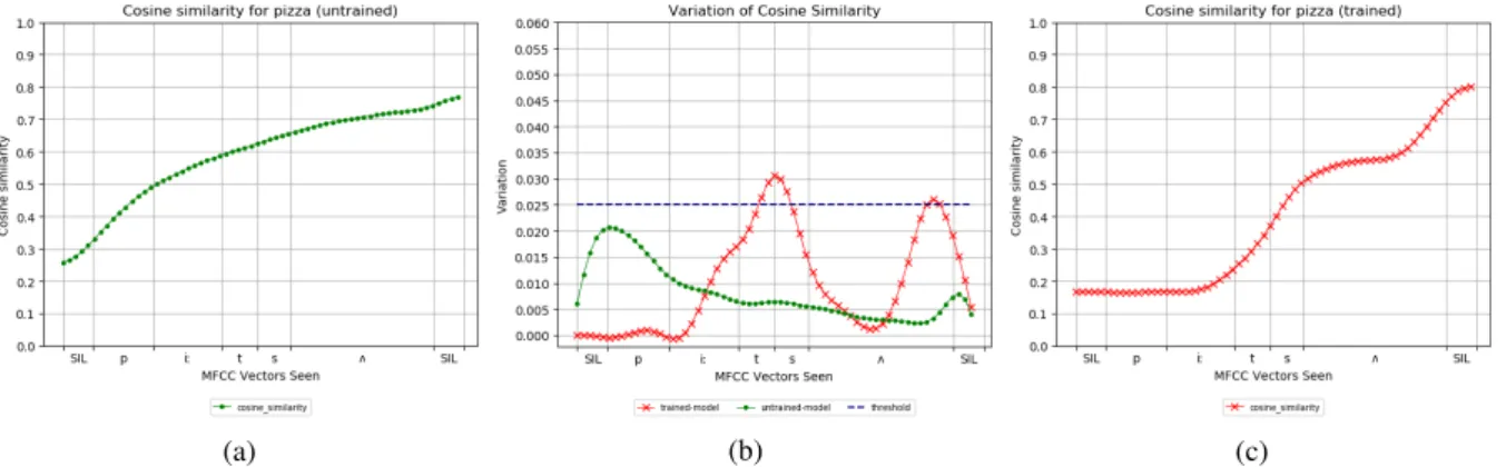
Figure 4: Evolution of cosine similarity for the word “pizza”. Figure4bshows peaks indicating the inflection points of curve4a(untrained model, green) and4c(trained model, red)
(a) (b) (c)
Figure 5: Evolution of cosine similarity for the word “scissors”. Figure5bshows peaks indicating the inflection points of curve5a(untrained model, green) and5c(trained model, red)
(a) (b) (c)
Figure 6: Evolution of cosine similarity for the word “sink”. Figure6bshows peaks indicating the inflection points of curve6a(untrained model, green) and6c(trained model, red)
(a) (b) (c)
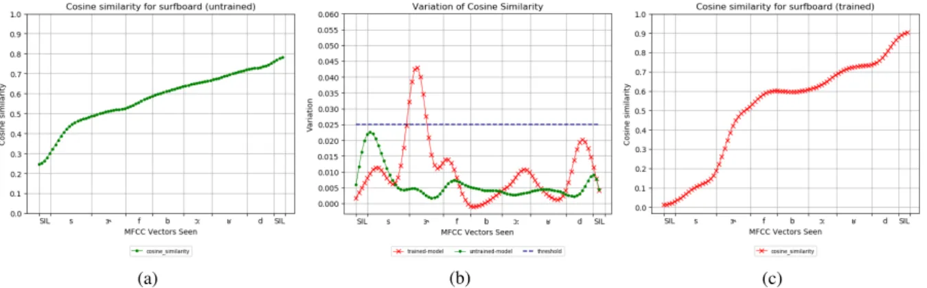
Figure 7: Evolution of cosine similarity for the word “surfboard”. Figure7bshows peaks indicating the inflection points of curve7a(untrained model, green) and7c(trained model, red)
(a) (b) (c)
Figure 8: Evolution of cosine similarity for the word “toilet”. Figure8bshows peaks indicating the inflection points of curve8a(untrained model, green) and8c(trained model, red)
(a) (b) (c)
Figure 9: Evolution of cosine similarity for the word “traffic light”. Figure9bshows peaks indicating the inflection points of curve9a(untrained model, green) and9c(trained model, red)
(a) (b) (c)
Figure 10: Evolution of cosine similarity for the word “train”. Figure10bshows peaks indicating the inflection points of curve10a(untrained model, green) and10c(trained model, red)
(a) (b) (c)
Figure 11: Evolution of cosine similarity for the word “wine glass”. Figure 11b shows peaks indicating the inflection points of curve11a(untrained model, green) and11c(trained model, red)
(a) (b) (c)
Figure 12: Evolution of cosine similarity for the word “zebra”. Figure12bshows peaks indicating the inflection points of curve12a(untrained model, green) and12c(trained model, red)
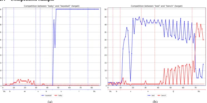
A.4 Competition Sample
(a) (b)
Figure 13: Competition plots between13a“baseball” and “baby” and13b“bed” and “bench”.
(a) (b)
(a) (b)
Figure 15: Competition plots between15a“meat” and “mirror” and15b“mirror” and “meter”.
(a) (b)