Computational reconstruction of images from optical holograms

(1)

Computational Reconstruction Of Images From Optical

Holograms

by

Weichang Li

Submitted to the Department of Ocean Engineering and

Department of Electrical Engineering and Computer Science

in partial fulfillment of the requirements for the degrees of

Master of Science in Ocean Engineering

and

Master of Science in Electrical Engineering and Computer Science

at the

MASSACHUSETTS INSTITUTE OF TECHNOLOGY

February 2002

Massachusetts Institute of Technology 2002. All rights reserved.

. ...

Department of Ocean Engineering

...

September 1, 2001

Certified by.

\jV

Accepted by ...

... ...

Jerome H. Milgram

W

Professor of Marine Technology

Thesis Supervisor

...

Henrik Schmidt

Chairman, Dep'artment Committee on Graduate Students

Read by ...

)2

ArthuV 1B. Baggeroer

, Ford Pjpfessor of Engineering

, Thesis Reader

Accepted by ...

Arthur C. Smith

BARKER

Author

MASSACHUSETTS INSTITUTE OF TECHNOLOGY

APR

IES

LIBRARIES

(2)

(3)

Computational Reconstruction Of Images From Optical Holograms by

Weichang Li

Submitted to the Department of Ocean Engineering and

Department of Electrical Engineering and Computer Science on September 1, 2001, in partial fulfillment of the

requirements for the degrees of Master of Science in Ocean Engineering

and

Master of Science in Electrical Engineering and Computer Science

Abstract

This thesis describes the analysis, development and implementation of computational re-construction of optical holograms, and its applications in marine biology and Holographic Particle Image Velocimetry (HPIV). Computational reconstruction of holograms is a pro-cess that recovers three-dimensional information from its holographic form computationally rather than optically. In this thesis, the reconstructions are represented by a sequence of plane images at programmable distances parallel to the associated hologram. The primary goal is to increase the reconstruction speed and improve the image quality, and ultimately lead to a computational platform that is efficient and robust for oceanographic applica-tions such as for marine biology and HPIV. A signal processing path has been followed throughout this thesis. Reconstruction algorithms have been developed in wavenumber space and accelerated by the use of FFT algorithms. Modifications to the reconstruction kernel both in spatial domain and frequency domain have been incorporated to improve the reconstruction quality. The behavior of reconstruction process is described qualitatively. A number of focus measures are proposed for quantitative focus analysis based on a circular disc object. Optimal sampling of holograms is also discussed and found to be distance-dependent. A PC based computational reconstruction system has been constructed which in addition consists of a commercial memory-enhanced DSP engine and a high-resolution scanner. As compared to optical reconstruction, by using this system the reconstruction time of one hologram has been reduced by a factor of 100 to 383.3 minutes for recovering

one 24.8mm * 24.8mm * 250mm volume at a resolution of 315pixel/mm. Both

simula-tion results of HPIV and experimental results of marine micro-organism are presented. A computationally efficient method has been devised for object-counting based on hologram images.

Thesis Supervisor: Jerome H. Milgram

Title: W. I. Koch Professor of Marine Technology

Thesis Reader: Arthur B. Baggeroer Title: Ford Professor of Engineering

(4)

(5)

Acknowledgments

I am more than grateful to my advisor, Prof. Jerry Milgram, for taking the gamble and

giving me the chance to work on this computational holography project, providing funds and guiding me through. I also wish to thank Prof. Art Baggeroer, for being my thesis reader on EECS part and providing insightful suggestions.

Lots of other people had provided help during the course of this thesis and deserve credits here. Thanks to Dr. Ed. Malkiel and Prof. Joseph. Katz of Johns Hopkins Univ. for providing all the optical holograms that have been used in this thesis. The discussion with Dr. Ed. Malkiel and Omar Alquaddoomi triggered the object counting part in this thesis. Also I would like to thank Dr. Edith Widder for sending me bioluminescence images, and Dr. Richard Lampitt for providing me the real corpepod image.

Thanks to Rick Rikoski for proofreading chapter 4 and 5, I know it is not easy.

Finally, I would like to thank my wife, Hua, for her unfailing support, both moral and practical, throughout the whole course.

(6)

(7)

List of Figures

2-1 Optical system used to record an in-line hologram; . . . 23

2-2 Optical system used to reconstruct the image from an in-line hologram; . . 24

2-3 Hologram recording with an off-axis reference beam; . . . . 24

2-4 Image reconstruction from an off-axis hologram; .. . . . .. 25

2-5 Block diagram of general holography recording and reconstruction, after lin-earization. For in-line holography, 0 = 0. (a) Holography recording process; (b) Holography reconstruction. . . . . . 31

2-6 Block diagram of the virtual image and the twin-image. For in-line hologra-phy, 0 = 0. (a) The virtual image; (b) The twin-image. . . . . 32

2-7 A three-dimensional object distribution . . . . 33

2-8 Scattering from an object distribution . . . . 34

2-9 Scattering from one object . . . . 35

2-10 The scattering from active regions on one slice of object . . . . 35

2-11 The object distribution of one slice of the volume . . . . 35

2-12 Spectra in one dimension for an image and its in-line and off-axis holograms a. Image, b. In-line hologram, c. off-axis hologram . . . . 38

2-13 Block diagram of the virtual image and the twin-image, with finite aperture effect. For in-line holography, 0 = 0. (a) The virtual image; (b) The twin-image . . . . 41

(10)

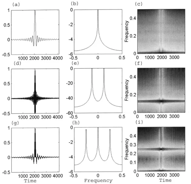
2-14 AM signals, spectrums and spectrograms

(a) a(t) = sinc(50t * f₅)rect(2048/f₈ ). (b) The normalized spectrum of a(t). (c) The Spectrogram of a(t)(Window length is 256/fS, step is 10/f,)

(d) The modulated signal s(t) = a(t)cos(27rf,/8t). (e) Spectrum of s(t). (f) The Spectrogram of s(t)(the same window length and step as in (c)) (g) The demodulated signal r(t) = s(t)cos(27rf,/8t). (h) Amplitude

spec-trum of r(t).

(i) The Spectrogram of r(t)(the same window length and step as in (c)) . . 44

2-15 ID holographic signals, spectrums and spectrograms

(a) a(f) = sinc(50fL). (b) The normalized spectrum of a(f).

(c) The Spectrogram of a(f)(Window length is 256/L, step is 10/L) (d) The modulated signal s(f) = a(f)cos(rAzof2), A = 633nm, zo = 100mm. (e) The spectrum of s(f). (f) The Spectrogram of s(f)(the same parameters as (c))

(g) The demodulated signal r(f) = s(f)exp(7rAzf2

), Zr = -ZO.

(h) Amplitude spectrum of r(f).

(i) The Spectrogram of r(f)(the same parameters as in (c)) . . . . 45

3-1 The Diagram of computational reconstruction . . . . 49

3-2 The bandwidth of a hologram of finite format; . . . . 51 3-3 Algorithm structure; (a) start with spatial kernel construction; (b) construct

frequency kernel directly. . . . . 57

3-4 Profiles of the virtual image of a circular object

(a) In focus; (b) Defocused by 6z. . . . . 60 3-5 the twin-image effect

(a) The profile of the twin-image associated with the focused virtual image;

(b) The total reconstructed image associated with focused virtual image. . 61 3-6 MSE focus measure verses misfocus distance

(a) Virtual image only; (b) Virtual image and twin-image . . . . 64

3-7 Energy focus measure verses misfocus distance

(11)

3-8 Gradient peak focus measure verses misfocus distance

(a) Virtual image only; (b) Virtual image and twin-image . . . .

3-9 The spatial window function . . . . 3-10 T he hologram . . . . 3-11 The frequency kernel with and without windowing (F is the sampling fre-quency) . . . . 3-12 Reconstruction with different window shapes in frequency domain

(a) the normal reconstruction; (b) window shape a = F/64;

(c) window shape o= F/32 (F is the sampling frequency). . . . . 3-13 The spatial kernel with and without windowing (L is the kernel size in one dim ension) . . . . 3-14 Reconstruction with different window shapes in spatial domain

(a) window shape

o-

= L/32;

(b) window shape o- = L/8 (L is the kernel size in one dimension). . . . . .

4-1 Conventional Optical Reconstruction System(courtesy of Dr. E. Malkiel) . . 4-2 DSP Based Digital Reconstruction System . . . .

4-3 DSP program flowchart . . . .

4-4 Single reconstruction time on different computing platforms . . . .

5-1 The 3D view of the volume . . . . 5-2 a. The plane view of the sample volume.

b. The central portion of (a) after enlarged by a factor of 4. . . . . 5-3 The hologram of volume without noise and its reconstructions

a. The hologram.

b. Reconstructed image plane at 99mm from the hologram. c. Reconstructed image plane at 99.5mm from the hologram. d. Reconstructed image plane at 100mm from the hologram. e. Reconstructed image plane at 100.5mm from the hologram.

(12)

5-4 The hologram of volume with noise density of 5 particles per mm3 and its reconstructions

a. The hologram.

b. Reconstructed image plane at 99mm from the hologram. c. Reconstructed image plane at 99.5mm from the hologram. d. Reconstructed image plane at 100mm from the hologram.

e. Reconstructed image plane at 100.5mm from the hologram.

f. Reconstructed image plane at 101mm from the hologram. . . . . 87 5-5 The hologram of volume with noise density of 2.4 particles per mm3 and its

reconstructions a. The hologram.

b. Reconstructed image plane at 100mm from the hologram. 88

5-6 Image Reconstructions from a hologram of a large copepod. a. Optical reconstruction (courtesy of Dr. E. Malkiel).

b. Computational reconstruction using the exact kernel.

c. Computational reconstruction using the paraxial approximation.

d. Computational reconstruction with twin image reduction. . . . . 92 5-7 Image reconstructions from a hologram of a linear diatom.

a. Optical reconstruction (courtesy of Dr. J. Zhang).

b. Computational reconstruction using the paraxial approximation. . . . . . 93 5-8 Image Reconstructions from a hologram of a helical diatom.

a. Optical reconstruction (courtesy of Dr. E. Malkiel).

b. Computational reconstruction with the hologram digitized at 126 pixels

per mm.

c. Computational reconstruction with the hologram digitized at 315 pixels per m m . . . . 94

5-9 Image reconstructions of a copepod whose center plane is at an angle to the reconstruction plane.

a. Optical reconstruction b: Computational reconstruction with the holo-gram digitized at 315 pixels per mm. . . . . 95

(13)

5-10 Summation of parallel planes through a holographic image, spaced 2 mm

apart.

a. Each image has intensity scaled to full range.

b. Analytic sum for Np, used. . . . . 98 5-11 The image of Figure 5-10b after low frequency removal . . . . 99 5-12 Result of applying an 0.38 threshold level to Figure 5-11 . . . . 99 5-13 Results of an 0.1 mm x 0.1 mm erosion process applied to Figure 5-12 . . . 100

5-14 The image of Figure 5-13 after dilation of each point to a square of dimensions

(14)

(15)

List of Tables

4.1 Number of real multiplications involved in one reconstruction, without

(16)

(17)

Chapter 1 Introduction

1.1 Overview

This thesis describes the analysis, development and implementation of computational re-construction of optical holograms, and its applications in marine biology and Holographic Particle Image Velocimetry (HPIV). Computational reconstruction of holograms is a pro-cess that recovers the three-dimensional information encoded in a hologram computationally rather than optically. In this thesis, the reconstructed results are represented by a sequence of plane images at programmable distances parallel to the associated hologram. The primary goal is to increase the reconstruction speed and improve the image quality, and ultimately to provide a computational platform that is efficient and robust for oceanographic applications such as for marine biology and HPIV. A signal processing path has been followed through-out this thesis. Reconstruction algorithms have been developed in wavenumber space and accelerated by the use of FFT algorithms. Modified kernel functions by spatial windowing and filtering have been incorporated to improve the reconstruction performance. The be-havior of the reconstruction process is described as a matched filtering. A number of focus measures are proposed for focus analysis. Optimal sampling of holograms is also discussed and found to be distance-dependent. A PC based computational reconstruction system has been constructed which in addition consists of a commercial memory-enhanced DSP engine and a high-resolution scanner. Both simulation results of HPIV and experimental results of marine micro-organisms are presented. A computationally efficient method has been devised for object-counting based on hologram images.

(18)

1.2 Holography, Computational Holography

The invention of optical holography was a result of an "exercise in serendipity", as Dr. Dennis Gabor explained in his autobiography. He proposed the principle of wavefront reconstruction in [6], followed by two more lengthy papers [7][8], mainly considering the possible applications of holography to microscopy. The technique attracted mild interest until in 1960s when the concepts and technology were dramatically improved, mainly due to the invention of the laser and the off-axis holography technique introduced by E. N. Leith and J. Upatnieks [4]. Its applicability and practicality were vastly extended, which leads to successes in a variety of applications. The quality and realism of three dimensional images obtained by holography led to the development of a great interest in the field.

Computational holography is about computational synthesis of holograms for later dis-play, or computational reconstruction of optical holograms. Computational synthesis of holograms began as early as 1964; researchers started to consider the computation, trans-mission and use of synthesized holograms to create images [23]. Early development of computational analysis of particle holograms [25] were often considered under far-field as-sumption which reduces the reconstruction to a modified Fourier transform. Barriers to get high-fidelity reconstruction computationally include the substantial computation capacity required to manipulate the tremendous amount of information embedded in a hologram, and the distortion and intrinsic noise inherent in the processes as well. In 1980's Onural and Scott [19] reported a method for the digital decoding of the in-line hologram, which is equivalent to a high order approximation that can reduce the twin-image effect. Unfor-tunately as the order increases, the resulted image quality is degraded by other artifacts. Computational reconstruction mainly involves the discretization of holograms, 2D Fourier transform, inverse transform and filtering. Most previous work is focused on computational implementation of optical processes, which is a good point to start, but not necessary the best solution for computational reconstruction. Instead of being viewed merely as computa-tional implementation of optical holographic processes, the problem can also be considered as a inverse problem to which appropriate signal processing operations can be applied.

(19)

1.3 Motivations for Computational Reconstruction of

Opti-cal Holograms

Holographic particle image velocimetry (HPIV) and underwater hologrammetry constitute the two major application fields of computational reconstruction of holograms. Particle image velocimetry(PIV) measures fluid flow field by measuring the velocity of particles in a fluid. HPIV is capable of doing 3D velocity measurement in one shot, hence is ideal for measuring complex high-speed flow such as turbulent flow. The other application of under-water hologrammetry has been mainly used by marine biologists to find out the individual morphology, population pattern and mutual dependence of marine micro-organisms such as plankton. These are well known to be an essential part of the food chain. As an noninvasive, in-situ and 3D imaging technique, holography has become a promising tool for marine biol-ogists, capable to provide the data necessary for the mathematical and conceptual modeling of the underwater ecosystem.

For all these and other applications, most of the present technology is photographic recording media. However, the real challenge lies in processing the huge amount of infor-mation contained in these holograms. Typically, it would take several days to reconstruct an object scene from one hologram using optical replay and high resolution digitizing systems. The laborious process can be unstable and inflexible. The image quality is influenced by optical abberations and limited by the replay setup. By computational reconstruction, the motivation is to develop alternative methodology and implementation systems that work computationally rather than optically, which are able to generate high fidelity reconstruc-tion in a short amount of time. The long term hope is the ultimate development of a film free digital recording and reconstruction system which, as we believe, will be more efficient and robust than current optical systems, and easier to operate.

(20)

(21)

Chapter 2 Modeling and Analysis of Optical

Holography

The principle and theory of optical holography have been well established since Dr. Gabor invented optical holography and published his pioneering work in [6][7][8], and has been vastly exploited in a broad range of applications after the invention of off-axis holography by E.N. Leith and J. Upatnieks [4]. Linear system treatment of scalar diffraction theory has also been well developed and can be found in Goodman's classical textbook on Fourier optics [10]. Therefore in this chapter we are not intending to present any new theory about optical holography. Rather, effort is made to formulate optical holography in a linear system frame and analyze it from signal processing perspective. A general formulation of both in-line holography and off-axis holography is proposed explicitly as a 2D linear convolution. This underlies the basis for computational reconstruction that will be discussed in subsequent chapters.

Optical holography, consisting of two steps including hologram recording and image reconstruction, is essentially a synthesis of interferometry and diffraction. A hologram as recorded, regardless of its media form, is a set of fringe patterns that results from the interference between an object wave and a reference wave. When being reconstructed, it manifests itself as a set of diffraction gratings. The associated diffracted field constitutes a reconstruction of the original object field. Generally in a typical holography setup, the object waves striking the hologram plane are the scattered waves from certain object sources. The recording of an optical field on holographic media such as film and plates is an intensity

(22)

mapping process. Therefore an optical hologram is an "energy detector" for the total interaction field. (Note that for long-wave cases such as acoustic holography and electronic holography, sensors are readily available for direct recording of a full wave field. Thus the holography technique of introducing a reference wave is not necessarily a startling achievement for long-wave cases.)

Both holographic recording and reconstruction are composed of a similar set of physical phenomena, namely interference and diffraction. Or as put by E. N. Leith and J. Upatnieks [4] in communications terminology, "a modulation, a frequency dispersion and a square-law detection". "Square-law detector" refers to the intensity mapping of a hologram recording. In addition to two linear data-containing terms, the intensity mapping also generates a

DC component and nonlinear terms which are not linear operations. The DC component

corresponds to transmitted reference light and can be eliminated in computational recon-struction. The nonlinear term is the object distribution intensity which is usually very weak and negligible if the reference wave is made much stronger than the object distribu-tion. Under these assumptions, the interference becomes bipolar and linear treatment is justified.

According to Fourier optics [10], the propagation of the optical field from an object space onto the hologram plane, or the diffraction from an object distribution to the hologram plane, is essentially a linear all-pass filtering process with a quadratic phase response under the paraxial approximation. It has also often called the Fresnel transform [11]. The Fresnel transform characterizes the propagation of an optical field in the Fresnel region which is a continuum transition field having mixed properties of both the object space and the Fourier space. Under far field assumption, the Fresnel diffraction degenerates into the Fraunhofer diffraction. Due to the simplicity of Fraunhofer diffraction, most applications assume the far-field criteria being satisfied [26], such as particle field holography and HPIV. Issues such as transverse and axial resolutions have usually been exploited under the same simplification [2]. However, the same issues in Fresnel region have rarely been discussed explicitly. The reason is because when the near field is being considered, the analysis becomes much more complicated. In this sense classical Fourier optics theory is somewhat far-field oriented.

This chapter is divided into two parts: formulation and analysis. Formulation is carried out in section2.1 for simple disc objects. It proceeds by treating holography as a combi-nation of bipolar interference (section 2.1.1) and diffraction (section 2.1.2). Ultimately the

(23)

general form is given in section 2.1.3, with extension to three dimensional object distribution discussed in section 2.1.4. In section 2.2, the analysis part is discussed. Based on Fourier optics and its physical realm, namely the plane wave decomposition and angular spectrum propagation, the finite hologram aperture effect is described. In addition an analogy of optical holography as a chirp carrier modulation has been established.

2.1 Linear System Modeling

In this section, we formulate both in-line holography and off-axis holography in a general mathematical representation. In the following discussion, the recording and reconstruction are covered simultaneously as they fundamentally embody the same set of physical processes.

2.1.1 Principle of Holography: Bipolar Interference

Holography is essentially an interference phenomenon, or a modulation process. In this section holographic recording and reconstruction are described mainly as wavefront encoding and decoding processes, for an arbitrary object distribution. The connection between the object wavefront and the associated object distribution will be explained in section 2.1.2.

Figures 2-1, 2-2, 2-3 and 2-4 show sketches of making holograms and reconstructing their optical fields for both in-line and off-axis holograms.

scattered w e diectly t ansmitted wave

Laser beam source object recording medium

Figure 2-1: Optical system used to record an in-line hologram;

Wavefront Recording

For both in-line and off-axis holograms, the optical field that falls upon the holographic film is the sum of a reference beam, r(Xh, Yh), and the object beam, o(xh, Yh). Xh and Yh are the

(24)

virtual image eal mage

Laser beam source hologram

Figure 2-2: Optical system used to reconstruct the image from an in-line hologram;

reference w ve sca tered wave

p1 ism

0

Laser beam source object recording medium

Figure 2-3: Hologram recording with an off-axis reference beam;

coordinates on the holographic film with the origin on the optical axis. The light intensity, I, which is what the film records, is the magnitude squared of the field.

I(Xh,yh) = r(xh,yh)+o(Xh,yh)l2

= jr(xh,yh)12 + jo(Xh,yh)|2 +r(xh,yh)o*(Xh,yh) -r*(xh,yh)o(Xh,yh)(2.1)

* indicates complex conjugate.

Of the four terms on the right hand side of equation (2.1), the first one is simply a constant, which has no consequence. The second term is an out of focus representation of the image, usually called the halo. The third and fourth terms are the optical fields of the real and virtual images multiplied by a constant for an in-line hologram and by a spatial sinusoid for an off-axis hologram. It is these last two terms that contain the optical field information we wish to capture and record. Generally, these terms are made much larger than the undesirable second term by making r much larger than o. For in-line holograms, we assume this has been done and ignore the first two terms. For off-axis holograms, we presume the off-axis angle is large enough to spatially separate the images from the halo

(25)

hologram prism source virtual image '-inl om - --real inage

Figure 2-4: Image reconstruction from an off-axis hologram;

and again the second term can be ignored. Therefore a bipolar form of I(xh, Yh) becomes:

I(xh,yh) =r(xh,yh)o*(Xh,yh) --r*(Xh,yh)o(Xh,yh) (2.2)

The description is given here in terms of the scalar theory of light (c.f. Goodman, 1996) [10]. An implicit aspect of the theory used here is that the functions refer to components of the reference and object beams that have the same polarization. For the representation of light waves, a time function of the form exp(-iwt) is implied and not written. The form of the reference wave is:

r(Xh, yh) = A exp(jkXh sin 0) (2.3)

where 0 is the off-axis angle with respect to the Xh axis, A is the uniform real amplitude. The reference beam is presumed to be perpendicular to the Yh axis. For an in-line hologram, 0 = 0. k is the circular wave number of the laser light beam.

If we assume [10]:

1 The variations of exposure in the interference pattern remain within a linear region of the tA vs E curve of the recording media.

2 The Modulation Transfer Function (MTF) of the recording material extends to sufficiently high spatial frequencies to record all the incident spatial structure.

3 The intensity A2 of the reference wave is uniform across the recording material. Laser beam

(26)

Then after dropping off any uniform bias transmittance, the amplitude transmittance of the developed film or plate can be written as:

th(Xh,yh) = 2/ARe{exp(ikXh sin )o*(Xh, yh)} (2.4) Where 3 is a constant related to the exposure time and the slope of the tA vs E curve.

Wavefront Reconstruction

Suppose that the developed transparency is illuminated by an reference light identical to the one used for recording. Then the light transmitted by the transparency becomes:

Ph(Xh,yh) = r(Xh,yh)th(Xh,yh)

= OA2 exp(j2kXh sin 0)o*(Xh, yh) + OA2o(Xh, yh) (2.5)

The first term is proportional to the conjugate of original object wave. It is deflected away from the optical axis at angle sin-1(2sin) and forms a real image field. The second term is the original object wave multiplied by a constant factor. It propagates along the optical axis and generates a virtual image field. Since 0 = 0 for in-line holography, all components are overlapped in space consequently. In off-axis case, it is possible to separate all these terms in space by increasing 0.

2.1.2 Diffraction and The Fresnel Transformation

In transmission holography, one common physical phenomena, diffraction, is shared by both the recording and the reconstruction processes. During recording, part of the reference wave is scattered by a source distribution in the object space and the scattered light reaches the recording media, interfering with the directly transmitted portion of the reference beam and being recorded. In the reconstruction phase, a reference light is incident on the holo-gram which is now equivalent to a diffraction grating, then the resulting diffraction field constitutes a recovery of the original wavefield. In this section, we formulate the diffraction field of a given 2D object distribution function as a linear convolution output. Without a paraxial approximation, the convolution kernel turns out to be as an exact kernel as given below. Under the paraxial approximation, the exact kernel degenerates into the Fresnel

(27)

transform kernel which is a pure quadratic phase factor.

Here we use the Huygens-Fresnel theory of diffraction as predicted by the first Rayleigh-Sommerfeld solution [10]. When illuminated by a normally incident uniform plane wave, the presence of two-dimensional object sources t,(xO, yO) across a plane F modifies the amplitude at an observation point P in the diffraction field to:

1 exp( jkr

o(P) = to(xo, Yo) cosO dxodyo (2.6)

Where A is the laser wavelength and k = 27r/A. E has coordinates (xo, yo, z) with z fixed. z = 0 at point P. r is the distance from point (X0, Yo, z) to point P. cosO is the so called

obliquity factor [10]. If we assume that P is a point on hologram plane with coordinates

(xh, Yh, 0), then r and the obliquity factor can be written as:

r = (Xh - xo)2 + (yh - yo)2 + z2

z

cosO = (2.7)

Therefore the object wave coming from the source and falling on the hologram becomes:

z

Z exp(jkv/(Xh - X") 2 + (Yh - Yo )2 + z2)dd (2.8)

jA At (Xh - XO)2 + (Yh - yo)2

) + z2

The above equation has the form of a 2D linear convolution:

O(Xh, Yh)

J

to(Xo, Yo)he(Xh - Xo, yA - yo; z)dxodyo

= {t(x, y) * *he (x, y; z)} =xh,y=yh _(2.9)

where ** means 2D linear convolution, and

he (x, y; z) = z exp(kx2 y2 z2) (2.10)

JA X 2+Y2 +z 2

Since the representation in equation (2.10) is derived exactly without approximation, we call he (x, y; z) as the exact kernel. It can be simplified using the paraxial approximation. If the lateral quantities (Xo - Xh) and (Yo - Yh) are small in comparison to the axial distance z, both the denominators and the arguments of the exponentials in equation (2.8) can be

(28)

approximated on this basis. The arguments of the exponentials must be carried out to one higher order in (X, - Xh) and (y, - Yh) to retain the crucial phase information. The resulting

expression for the field on the hologram, op is called the paraxial approximation and is given

by:

op(Xh,Yh) expjkz) to(Xo, yo)exp( [(Xh - Xo)2

+ (Yh - yo)2])dxzdy, (2.11)

If we let

hj(x, y; z) = exp[k (X2 + y2 j( 2 + y

2_)]

(2.12)

Then

Op(Xh, Yh) JA to(xo, Yo)hf (xh - Xo, yh - yo; z)dxodyo

= {to(x, y) * *hf (x, y; z)} x=-hYYh (2.13)

where the constant phase factor exp(jkz) has been dropped off since it has no consequence to reconstructed images.

hf(x, y; z) is a 2D chirp function and has a quadratic phase structure. It is usually called the Fresnel transform kernel. One nice property of the Fresnel kernel is that its Fourier transform is analytically available and is also a 2D chirp function in the spatial frequency domain.

Hf(fx,fy;z) = F{hf(x,y;z)}

= exp [-j7rAz(f2 +

f2)2

(2.14)

Corresponding to the concept of instantaneous frequency of a time signal, we define the local spatial frequency here as the derivative of the phase:

(

ia( (x2 + y2)) X fX W Az

1 ( (X2 + y2))

fy (y) = z (2.15)

We can further define the chirp rate as the derivative of the local frequency regarding the associated coordinate. Basically the chirp rate is the rate at which the frequency changes

(29)

with spatial variables and it is the same for both x and y directions in this case. By definition, its value is C, = 1/(Az). Note that Az is the characteristic length of diffraction

in optics. We can notice that the Fresnel kernel has a linearly modulated local spatial frequency whose modulating rate is Cr. Obviously C, decreases as z increases for fixed value of A.

It is easy to see that the Fresnel kernel function is neither spatially limited nor band limited. From equation (2.15), we can find that if it is spatially truncated, the maximum local frequency of hf(x, y; z) is dependent on the truncating window size, and also increases as the value of z decreases. This property will be used later to determine the sampling rate and spatial extent of the discrete kernel function in section 3.1.

A number of other properties of the Fresnel kernel that worth to be mentioned here, which are very helpful for the intuitive understanding of the diffraction process.

First, the form of H(fX,

fy;

z) implies that the Fresnel kernel is cascadable, i.e:

Hf (fX, fy; z1)Hf (f., fy; z2) = Hf (f, fy; z1 + z2)

hf(x,y;zl) **hf(x,y;z2) = hf(xy;z1+ 22) (2.16)

Consequently,

Hf(f.,fy;z)H(fx,fy; -z) = Hf(f, fy;0) =1

hf(x,y;z) * *hf(x,y;-z) = 6(x,y) (2.17)

Also h*(x, y; z) = hf(x, y; -z).

Second, the convolution of hf(x, y; z) with a uniform plane wave A exp[j(kxsinO

+

kysirnf3)] whose directional cosine is (sinO, sin/) becomes

Hf(fo, fy; z).F{A exp[j(kxsirnO + kysin3)]} H (fx, fy; z)A(fx - "n, fy - S-0)

exp -j7rAz( [,i]2 + [1i'3]2) A6(fx - , fy - SnO)

(2.18)

(30)

the directional cosine:

hf (x, y; z) * *A exp[j(kxsinO + kysin#3)]

SA exp[j(kxsin9 + kysin)] exp -j7rAz([{si]2 + [sij3]2)] (2.19)

Furthermore, the convolution of a constant A with hf(x, y; z) gives A itself.

Hf (fs, fy; z)A6(f., fy) = A6(fz, fy)

hf (x, y; z) * *A = A (2.20)

This intuitively makes sense because the free-space propagation of a uniform plane wave should change nothing to the wavefront.

2.1.3 Formulation of Holographic Recording and Reconstruction

Now we can combine the results of both section 2.1.1 and section 2.1.2 to generate a mathe-matical formulation for the whole process. Again we start by considering a two-dimensional object distribution t,(xo, yO; zO) which is located at z = z, and parallel to the hologram plane. The expression of the associated hologram can be derived by substituting equation

(2.8) or (2.13) into equation (2.4) :

th(Xh, yh; zo) ={A exp(jkx sin 0)[t* (x, y; z,) * *h*(x, y; zo)]

+OA exp(-jkx sin 0)[to(x, y; zo) * *h(x, y; zo)]} x=h (2.21)

Where h(x, y; z,) = he (x, y; zo) without the paraxial approximation, otherwise h(x, y; zo)

hf (x, y; zo).

Similarly by substituting equation (2.8) or (2.13) into equation (2.5), we can express the light transmitted through the hologram (at z = 0) as:

Ph(Xhyh; zo) = {A 2 exp(2kxsin)[t(x, y; zo) * *h*(x, y; zo)

+3A2[to(x, y; zO) * *h(x, y; zo)]} x=xh,Y=Yh _(2.22)

Where again h(x, y; zo) = h,(x, y; zo) without paraxial approximation, and h(x, y; z,)

(31)

Aexp(j kx sih3 )

t O(,Y (x,y7 x e t h(x,y;zo)

(a)

A expaj k x sihU )

t h(x,y;z ) X Ph (x, y ; zo) h~~;,Pr (x, y , zr "

(b)

Figure 2-5: Block diagram of general holography recording and reconstruction, after lin-earization. For in-line holography, 0 = 0.

(a) Holography recording process; (b) Holography reconstruction.

The optical field at z = z, due to the transmitted light Ph at z = 0, simply becomes: Pr(xr, yr; Zr, Zo) = {Ph(X, y, Zo) * *h(x, y; z,)} Ix=x,,y=y,

C{{exp(j2kx sin 0)[t*(x, y; zo) * *h*(x, y; zo)]} * *h(x, y; zr) +{[t₀(x, y; z0 ) * *h(x, y; z,)]} * *h(x, y; z,)} ix2xr,YYr

(2.23)

Where C = A2. Block diagrams corresponding to equation (2.21) and (2.23) are both

given in Figure 2-5.

If in addition Zr = -zo, then

Pr(xr,yr;zr,zo) = C{{exp(j2kx sin 0)[t*(x, y; zo) * *h*(x, y; zo)]} * *h(x, y; zr)

+t0(x, y; z0)} ix,,Y=yyr (2.24)

Equation (2.24) essentially says that when reconstructed at z, = -z, the field shows a

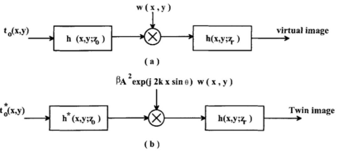
focused virtual image and a real image with a different focus which is usually called the twin-image. Both the virtual image and the twin image components are related to the object distribution as shown by the block diagrams in Figure 2-6.

(32)

t 0(x,y) virtual image

-- + h (x,y;g ) _{h(x,y;g )}

( a ) PA exp(j 2k x sito )

t

**e*(x'y)**

hTwin image

(b)

Figure 2-6: Block diagram of the virtual image and the twin-image. For in-line holography,

0 = 0.

(a) The virtual image; (b) The twin-image.

Now we consider in-line holography only. Since 0 = 0, the twin image overlaps the virtual image in an axial view and manifests itself as an extraneous ghost image. From equation (2.21), if the object distribution is purely absorbing, i.e. t,(x, y; zo) is real, then

after dropping all constant factors, th(Xh, yh; z,) can be written as

th(Xh, yh; Zo)

Th(f , fy; zo)

= {to(x, y) * *Re{h(x, y; zo)}} XIX=h,Yyh = {t0(x, y) **{zsin[7<X2 + y2_)]}}

x=xh Y=Yh = T0(f-,fY)H(f2,fY)= T0(f",fy)cos [rAzo(f2 +

f2)

The reconstructed field p,(xr, y,; z, zo) becomes:

Pr (ryr; zr, zo) {th(x,y;Zo) * *h(x,y;zr)} cr=X,,y=Yr {t*(x, y; zo) * *h(x, y; zr - zo)

+ t₀(x, y; zo) * *h(x, y; zr + z0)} IX=Xr,Y Yr

(2.26)

2.1.4 Extension To 3D Object Distribution

One might have already found that so far all discussions are based on a disc object model. We have talked about the recording and reconstruction of a hologram associated with an object distribution across one plane, which is located at a fixed distance and parallel to the

(33)

Figure 2-7: A three-dimensional object distribution

hologram. The axial extension of that plane object distribution has not been included in our consideration. However, in real applications, it is often an assembly of small objects, or particles that are involved when a hologram is taken. Each object has physical extension in all directions. Thus a hologram is a record of the wavefield from a three-dimensional object distribution rather than one simple object plane. In such cases, the interpretation of the physical meaning of a hologram and its reconstruction becomes much more complicated than in the disc object cases. Nevertheless, this three-dimensionality is what holography can provide us with.

In this section, we first clarify all the assumptions that we would have to impose upon the object distribution, the wave media and the scattering process, so that for a 3D ob-ject distribution, we can still use all the derivations from previous sections based on a disc object model. It will be shown that under these assumptions, a hologram of a 3D object distribution can be approximated by the superposition of holograms contributed by a se-quence of disc object distributions. Then an idealistic description of the scattering process throughout the object distribution will be given aiming to explain the information that is contained in a hologram and subsequently expressed by its reconstruction.

First of all, we assume that the object distribution consists of a sparse assembly of small particles contained inside a transparent three dimensional volume. The particles are assumed to be opaque and with some pure absorption. The medium inside the volume is a homogeneous free space other than the presence of particles. The reference light is assumed to be a strong collimated uniform laser beam which has already been polarized.

The scattering occuring in the object distribution is a complicated physical phenomenon. To simplify our discussion, we use assumptions according to the convention [13]. First, we

(34)

Single scattered light

Multi-scatr

6 4 .r-a4a 4a*~ 41 & & 4 4

Transmitted light.

Figure 2-8: Scattering from an object distribution

neglect Muti-scattering. Only the single scattered from each object is considered. Secondly, we neglect the extinction caused to the reference light when it propagates through the medium. Thus all objects are illuminated by the same uniform reference light. Third, all objects are assumed to be have pure absorption, therefore there is no change of polarization and frequency in the scattered light. Finally we assume independent scattering. It means that the phase difference between lights scattered from different objects are not correlated due to the randomness of the distribution. This assumption allows us to sum up all the scattered light in intensity without considering mutual interference.

In summary, all these idealistic assumptions entitle us to consider only two types of wavefield in front of the hologram plane. One is the transmitted reference light which suffers little distortion as we assumed; the other is the total single scattered field contributed by all objects. Therefore, the dominating component of the recorded field becomes the interference between these two waves.

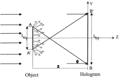
Let's then take a look at the scattering field originated from one object illuminated by the reference light. Figure 2-9 shows that the object body can be divided into three regions associated with different scattering properties: the backward scattering region, the forward scattering region and the geometrical shadow region. Among these three regions, only the information of the forward scattering region reaches the hologram and thus is recorded. We call this region the active region.

Now if we cut the object into many thin slices along the depth direction, as shown in figure 2-10, it is possible to represent the total scattering field by a superposition of contributions from the active region on each slice. At each slice plane, we can use the

(35)

s ca tterng

Geonetric Sh ow

Fo d Itin Holora

Figure 2-9: Scattering from one object

d

Figure 2-10: The scattering from active regions on one slice of object

LP _dz

Figure 2-11: The object distribution of one slice of the volume

F 0 !'W A

B .k d

(36)

distribution function representation for the scattering field as in previous sections. We then go back to the large picture of an assemble of particles. We use the same slicing operation which divides the whole volume into many slices. As assumed, the same reference light is assumed for all slices. We then characterize the scattering by objects inside each slice by a distribution function o(x, y; z), which is defined as the ratio of the complex amplitudes at the two sides of the slice in the proximity of point (x, y, z). Figure 2-11 shows a sketch of the slicing operation in a volume.

According to our assumption, the mutual interference between waves from different object slices are independent. The hologram is essentially a linear superposition of their interference with the reference light. Then an hologram of a 3D object space thy(3h,Yh)

can be represented by integrating th(X, y; zO) along zo:

thv (Xh, yh) Jth (Xh, Yh; zo)dzo (2.27)

Taking thy for reconstruction, the resulted field can be represented as an integration of

Pr (Xh, yh; zr, zo) regarding zo.

Prv (Xh, Yh; Zr) Pr (Xh, Yh; Zr, zo)dzo (2.28) When reconstructed at one particular distance z, the output consists of one in-focused image of the object plane at zr and the out of focus image of all other planes, together with all twin-images.

The limits of the validity of this object model depends on the object geometrical shape and scale normalized by the wavelength, and the distance between the object and the hologram as well. A good interpretation of reconstruction images relies on the actual scattering physics.

2.2 Observation and Analysis

From the perspective of computational reconstruction, we are interested in getting high-fidelity recovery of the original object distributions. It will be difficult to define a single deterministic measure for perfect reconstruction. As for our current representation form of the reconstructed field, there are a number of measures for image quality evaluation,

(37)

including the transverse and axial resolutions, the degree of distortion and the signal to noise ratio. Note that an image scoring high in terms of any one of these measures is not necessarily the best for human eye's observation. The resolution limit of the reconstructed field is closely tied to the information loss during the whole process. It is especially limited by the phase ambiguity and the effective hologram aperture. For in-line holograms, the noise mainly comes from the twin-image, the intrinsic speckle noise, and from out of focus particles or objects.

In this section, the finite aperture effect and the twin image interference will be discussed. In section 2.2.1, The ideas of the plane wave decomposition and the angular spectrum are briefly reviewed. The finite aperture effect can be described using a convolution expression. In section 2.2.2, in-line holography is described as an analogy to modulation in which the carrier signal is a 2D chirp function. In this sense the twin-image can be represented as a high chirp rate component.

2.2.1 Plane Wave Decomposition, Angular Spectrum Propagation and Finite Aperture Effect

The frequency domain equivalent of equation (2.9) and (2.13) is:

Oh(fx, fy) = To(fx, fy, ; zo)H(f1 , fy; zo) (2.29)

Where Oh(fx,

fy)

and T,(fx,

fy;

z,) are the Fourier transforms of the diffraction field and the object distribution respectively, or the angular spectrums. According to Fourier Op-tics theory [10], the angular spectrum of an optical field is its plane wave decomposition, with each spatial frequency pair (fx,

fy)

corresponding to a plane wave propagating in the direction specified by the direction cosine of (Afx,Afy, 1 - (Afx)2 -

(Afy)

2)). Therefore, according to (2.29), the propagation of an optical field simply becomes a dispersive pro-cess with a quadratic phase response as specified by equation (2.14), under the paraxial

approximation.

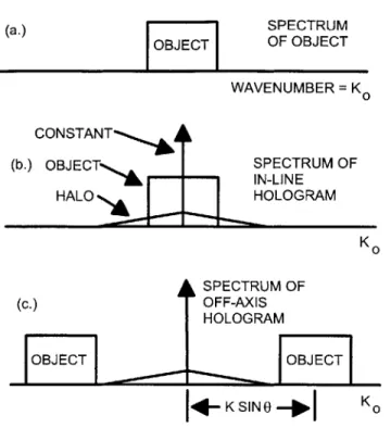
Figure 2-12 contains a sketch of an arbitrary angular spectrum in one direction as well as the components of the spatial spectra of its in-line and off-axis holograms. If the spectrum of the halo is small in comparison to the spectrum of the objects being encoded, the spatial sampling frequency of the in-line hologram must be twice the highest frequency

(38)

(a.) SPECTRUM

OBJECT OF OBJECT

WAVENUMBER = K₀

(b.) OBJECT CONST NT _LN-LINESPECTRUM OF

HALOsk HOLOGRAM K ₀ SPECTRUM OF (C.) OFF-AXIS HOLOGRAM OBJECT OBJECT I*-KSIN 0-o. K0

Figure 2-12: Spectra in one dimension for an image and its in-line and off-axis holograms a. Image, b. In-line hologram, c. off-axis hologram

in the image to satisfy the sampling theorem. It seems that only a modest advantage

from a higher sampling frequency since the halo represents "noise" whether or not it is aliased. In practice, the relative intensity of the halo is minimized by making the reference beam intensity large in comparison to the object beam intensity, when possible. For an off-axis hologram, if the off-off-axis angle is large enough to separate the desired phase encoding from the halo the required sampling frequency is four times larger than the required in-line frequency, and if the angle allows halo noise, but just separates the twin images, the required frequency is two times the needed in-line frequency. These increases apply to only one of the two directions on the hologram since the off-axis modulation is in only one direction.

Though H(fs,

fy;

z,) _{is an all-pass filter which is neither band limited nor space limited,} the actual recordable field is limited in spatial extension by the hologram size and reference beam span. Therefore information loss happens when an hologram is recorded. For sim-plicity, first we define an effective hologram aperture as the minimum of the reference beam span and the physical format of the recording medium. This effective hologram aperture stands for the maximum spatial extension of the recordable holographic information. It can

(39)

be included into consideration by simply imposing a window on the hologram. That is

th(Xh, yh; Zo) = w(Xh, yh){to(X, y) * *Re{h(x, y; zo)}} IX=xh,y=yh

where w(Xh, Yh) is the window function. It can be circular symmetric:

w(Xh, yh)

{

10 x + y; < R otherwise Or in a rectangular form: w(Xh, yh) 0 if Xh < R and Yh < R otherwise

Now let's check the field reconstructed from the windowed hologram. After including the effective finite aperture window, equation (2.26) becomes

Pr (Xr, Yr ; zo) = {{w(x, y) [to (x, y) * *Re{h(x, y; zo)}]} * *h(x, y; Zr) x=x,,y=y,

1

S{{w(x, y)[to(x, y) * *h(x, y; zo)]} * *h(x, y; zr)} IX=Xr,Y=Yr

+ 1f{{w(x, y)[to(x, y) * *h*(x, y; zo)]} * *h(x, y; zr)} Ix=x,,y=y,

- u1 + U2 (2.31)

Where u1 and U2 denote the virtual and real image component respectively.

We are mainly concerned about the effect of this finite aperture on the focused virtual image. Since the twin-image component U2 is an interference term anyway, we only discuss the effect on ui here. Expressed in an integral form, ui becomes:

Ui ffJ W (h, Yh) o(X, Yo)(Xh - Xo,yh yo; zo)dxodyo h(xr - Xh, Yr - Yh; Zr)dXhdYh

2 00

Jf

to(xo, yo) w(xh, Yh)h(xh - xo, yh - yo; zo)h(xr - Xh, Yr - Yh7 zr)dXhdYhdxodyo

2 _f 0

(2.32)

Let z= -z, and substitute hj(x, y; z) = exp

j(x

2_{+ y}2_{) into above, u}

1 becomes: (2.30)

(40)

U =2A2 2

JJ

to(o,yo) exp{j (X 0 - xr + yo - y)}

0" 27r

{

w(Xh, Yh) expfj A [Xh(Xr - Xo) + Yh(Yr - yo)1}dXhdyh}dxodyo

c o (/, yo) exp{j (x -X + y -Y )}W( (Xr -co), (y - yo))dxodyo

0~z ry0))dxzody (Y -z ₀

(2.33)

Where W( (Xr - Xo), '(Yr - yo)) is the 2D Fourier transform of the window func-tion w(Xh,yh). If the window size is infinitely large, i.e. w(Xh,yh) = 1, then W( f-(r

-co), ?j'(y, - yo)) becomes 6(Xr - Xo)6(Yr - y,), therefore,

1 o/o

S=- 00 to(Xo,Y o5)(x, - Xo)(Yr - yo)dxody,

2 iio 1

= to(xr,Yr) (2.34)

which means the virtual image is a perfect reconstruction. However when w(Xh, Yh) has finite support as in all real applications, the reconstructed virtual image is not a perfect reconstruction of the original object distribution. Rather it is an phase modulated object distribution convolved with the Fourier transform of the windows function. When the window size is large relative to VAZ, W( 2(Xr - Xo), Z(Yr - Yo)) is very close to J(xr

-Xo)j(yr - yo), thus the finite aperture effect is negligible. With the finite aperture effect included, block diagrams of virtual image and twin-image should be modified into Figure 2-13.

2.2.2 Chirp Carrier Modulation

In this section, we will describe the twin-image effect of in-line holography using an analogy to the well-known amplitude modulation (AM) process. We will show that due to the natural of the image component, it is very difficult to separate the virtual image and the twin-image using traditional filtering techniques, if not impossible. Recall that in communications an AM signal s(t) is generated by multiplying a modulating signal a(t) with a carrier signal

(41)

t O(x'y) hvirtual image

(a)

PA 2exp(j2kxsino) w(x,y)

t O(x9y) 1Twin image

(b)

Figure 2-13: Block diagram of the virtual image and the twin-image, with finite aperture effect. For in-line holography, 0 = 0.

(a) The virtual image; (b) The twin-image

c(t) = cos(wet), w, is the carrier frequency. That is

s(t) =_ a(t)cos(wet) (2.35)

At the receiver end, the received signal is r(t) = s(t) + n(t), where n(t) is the additive noise. An estimation of a(t) can be extracted from r(t) by demodulation, that is, first multiplying r(t) by the same carrier signal c(t) and then doing low-pass filtering, as shown below:

h(t) = {r(t)cos(wet)} * h(t)

= {a(t) * cos2(wet) + n(t) * cos(wct)} * h(t)

1 1

{a(t) + -a(t)cos(2wet) + n(t)cos(wet)} * h(t) (2.36)

2 2

Where h(t) is the impulse response of the low pass filter, so that the baseband components including a(t) can be separated from the high-frequency component a(t)cos(2wct).

Recall the expressions of the hologram Th(fo,

fy;

zo) and its in-focus reconstruction

pr(fx, fy; -zo, zo) given in section 2.1.3, their forms are analogous to those of s(t) and &(t).

This suggests an analogy between in-line holography and AM modulation. In equation

(2.25), the spatial spectrum of an hologram is the product of the angular spectrum of

the object and cos 7rAzo(f, +

f')J,

the angular spectrum of the kernel. The kernel can be thought of as the carrier signal and the object spectrum as the modulating signal. Therefore

(42)

in this sense the recording of a hologram becomes a modulation process in angular frequency domain. Since the carrier signal here is a chirp function, we call it chirp carrier modulation. The reconstructed field, as formulated in equation (2.26), is equivalent to the demodulated output. Therefore, the two steps process can be described in frequency domain as:

1. Modulation.

Th(f ,f,;z) 2T(fxfy)cos [rAzo(ff +

f2)

(2.37)

2. Demodulation.

Pr (fx, fy; zr -zo) = Th(fx,

fy;

zo) exp{j 7rAz (2 + f 2)}

= 2TO(f., fy)cos [7r Azo(f, +

f )]

exp{-j

[rAzo(fi

+ f)

}

= To(fx, fy) + To(fx, fy) exp{-j [27rAzo(fi + f )I} (2.38)

From equation (2.38), we can see that the twin-image is a chirp signal whose chirp rate is twice of that of the carrier signal. This is similar to the high-frequency term we got in AM demodulation. Though the whole process is analogous to AM modulation and demodulation, holography is different from AM in several aspects:

First, unlike in AM where single tone carriers are often used, in in-line holography the equivalent carrier signal is a 2D chirp signal with a quadratic phase structure.

The second difference is a direct consequence of the first one. In AM, the demodulated original signal is separable from other components in frequency domain and thus can be extracted simply by low-pass filtering. Unfortunately this is not the case for in-line hologra-phy. The result in equation (2.38) indicates that the two components are separable neither in spatial domain nor in frequency domain. The two components are different only in their chirp rate(see definition in section 2.1.2): C, = 0 for the virtual image and Cr = 2/(Azo) for the real twin image. If there is a way to transform pr into the chirp rate domain and if the transform is invertible, then the two terms can be separated by doing filtering in the C, domain.

To visualize this analogy, Figure 2-14 and Figure 2-15 have illustrated the signals, their spectrums and spectrograms in an AM process and an in-line holography process respec-tively. Figure 2-14a, b, c show the waveforms, spectrums and spectrograms of the

Computational reconstruction of images from optical holograms