Comparison Of Scattered Energy Using Point Scatterers Versus Full 3D
Finite Difference Modeling
Mark Willis, Yang Zhang, and Daniel Burns Earth Resources Laboratory,
Dept. of Earth, Atmospheric and Planetary Sciences Massachusetts Institute of Technology
Cambridge, MA 02139
Abstract
We present results of 3D numerical modeling using a series of simple point scatterers to create synthetic seismic shot records collected over regular, discrete, vertical fracture systems. The background medium is taken to be constant velocity. The model contains a series of point scatterers delineating the top tip and bottom tip of each vertical fracture. We use these results to gain an understanding of some of the features seen in full 3D elastic modeling of vertical fractures. We compare our results to those of Willis et al (2003) and Willis et al (2004) for their 5 layer model with 50m spacing between discrete, vertical fractures. Our modeling shows that a series of back scattered events with both positive and negative moveouts are observed when the shot record is oriented normal to the direction of fracturing. When the shot record is both located in the middle of the fractured zone and is oriented normal to the direction of fracturing, a complicated series of beating is observed in the back scattered energy. When the shot record is oriented parallel to the fracturing, ringing wavetrains are observed which moveouts similar to reflections from many horizontal layers. The point scattering models are, in general, very consistent with the full 3D elastic modeling results.
1. Introduction
Previous studies (Willis et al, 2003; Willis et al; 2004) modeling regular, vertical discrete fracture systems show many complicated patterns of scattering. It is difficult to know from the full 3D elastic modeling results whether the energy observed is P wave energy scattered back to P wave energy or back to S wave energy. One would think that travel times alone should be sufficient to determine something as seemingly simple as this. However, the complicated wave trains are difficult to decipher by themselves. In order to more fully understand the mechanics and gain insight into the processes that create these patterns of scattered energy, we use a much simpler model and modeling method.
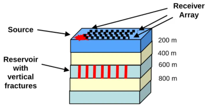
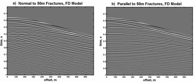
We attempt to mimic the qualitative nature of the models developed by Willis et al (2003 and 2004) which are shown in Figure 1 and Table 1. Their models contain five layers in which the middle layer has vertical fractures. This center layer is 200-m thick and contains parallel, vertical fractures which are as tall as the layer, one grid cell thick (5m) and run the entire width of the model. They modeled five different fracture spacings, including 50m, but we limit our discussion here to only the case with vertical fractures spaced 50m apart. They used the 3-D elastic finite difference code, developed by Lawrence Berkeley National Laboratory (Nihei et al., 2002), to synthesize all reflections and scattered energy. Figure 2 shows the shot records oriented (a) normal and (b) parallel to the fractures. It is clear on the shot record normal to the fracture direction that there is no coherent stackable energy in or below the reservoir level (300 ms). However, for the parallel case, there are many coherent events that can be seen primarily below the base reservoir reflection on the shot record and observed on the velocity analysis. In the direction parallel to the fractures, the seismic energy seems to be guided by the aligned fractures and the resulting scattered energy is more coherent and similar to the direct P wave reflection.
Receiver
Figure 1. Diagram showing the geometry of the 3D finite difference model used by Willis et al (2003 and 2004). The layer velocities and densities are shown in Table 1. The source is located in the left front corner (red symbol) and the receivers are spread out in a rectangular area 1000 m wide and 1000m deep. The receiver spacing is 5m in each direction.
Table 1. Parameters for model
Layer Thickness (m) Vp (m/s) Vs (m/s) Density (g/cc)
1 200 3000 1765 2.2 2 200 3500 2060 2.25 3 200 4000 2353 2.3 4 200 3500 2060 2.25 5 200 4000 2353 2.3 Array Source 200 m 400 m Reservoir 600 m with vertical 800 m fractures
Figure 2. Vertical component of the 3D Finite difference modeling for 50m fracture spacing from Willis et al (2003 & 2004): a) shows the shot record acquired normal to the fractures, b) shows the shot record acquired parallel to the fracture direction.
2. Modeling
For our modeling we used a much simpler approach consisting of a constant velocity medium and a method which makes no corrections for spreading or attenuation. The P wave velocity used is 4000 m/s and the S wave velocity used is 2353 m/s. Figure 3a shows the diagram of an array of receivers on the surface of the ground, spaced 5m apart in both x and y directions and shown in black triangles. Below the surface are located two sets of identical fracture systems, represented by a series of point scatterers. The first set is located a depth of 400m. The second set is located at a depth of 600m. These sets of scatterers are intended to mimic the top tip and bottom tip of each fracture in Figure 1. The extension of the fracture in the y direction is modeled by closely spaced point scatters to simulate the continuous edges of the fracture in that direction. In the x direction, the scatterers are spaced apart at 50m, representing the distance between the fractures.
To create each seismogram, we utilize a Huygens-type approach in which each scatterer acts as a point source which is time delayed by the one way travel time from the shot location to the point scatterer. Each synthetic trace is simply the summation of the contributions from each of the scatterers. This amounts to repeatedly summing together a 40Hz Ricker wavelet delayed in time by the total time from the source down to each scatterer and then up to the receiver. The model itself contains no reflectors other than the point scatterers and we assume no secondary scattering.
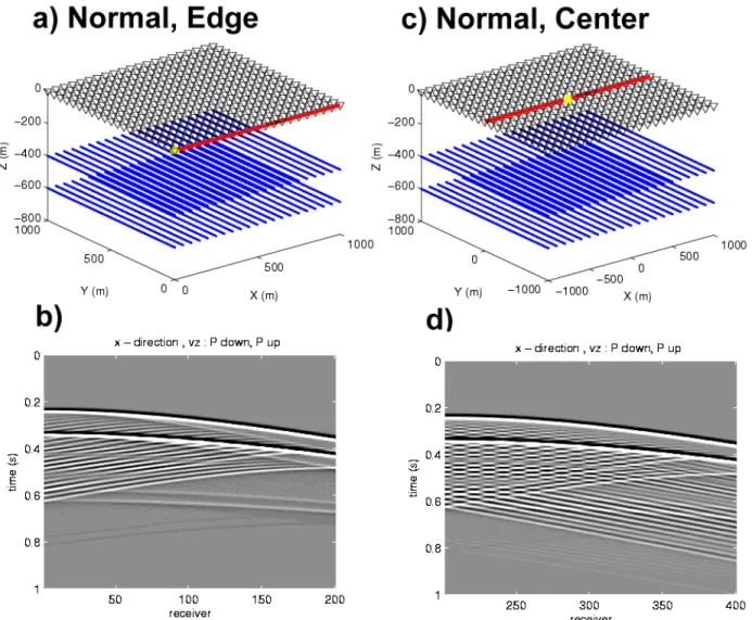
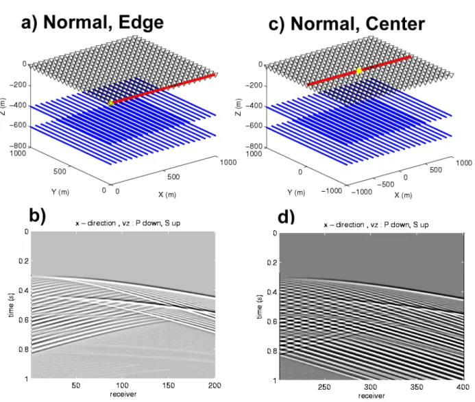
We first examine P-P scattering representing a P wave source which is converted to P wave energy by each point scatterer. The seismograms for P-P scattering recorded at the front edge (y=0) of fracture model, acquired normal to the fractures, are shown in Figure 3b. The source is located at the origin (x=0, y=0) which is shown as a yellow symbol. The red line in Figure 3c corresponds acquiring a shot record in the middle of an area with fractures. The corresponding P-P shot record is shown in Figure 3d. Since this model does not contain any continuous reflectors or layering, the constructive interference of the scatterers themselves forms what seems to be strong primary and secondary arrivals in both the edge and centered acquistions. Note how on both records, most of the ringing, scattered energy is seen later in time than what appears to be the second event. Also evident on the centered seismogram (Figure 3d) is a strong lateral beating phenomenon corresponding to the back scattering from fractures located symmetrically on both sides of the source.
Figure 3. Vertical component of simple P-P diffractor model with a receiver line (red) normal to the fractures. a) model geometry of shot at edge of fractured zone, b) the simulated waveforms acquired at edge of fractured zone, c) model geometry of shot in center of fractured zone, d) the simulated waveforms acquired in the center of the fractured zone. Each trace is spaced 5m apart.
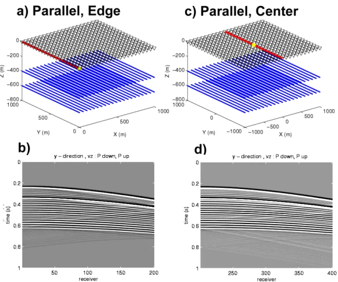
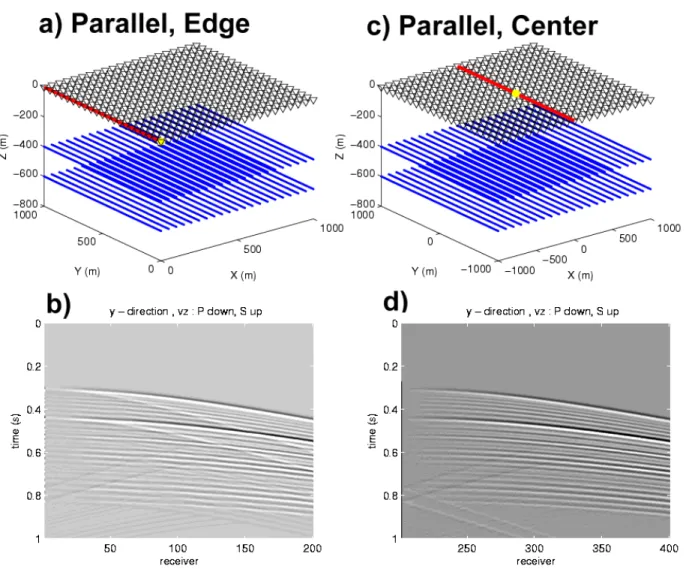
Still looking at P-P scattering, we next examine the case of acquiring shot records parallel to the fracture orientation. The seismograms are shown in Figure 4b for P-P scattering observed from the left edge (x=0) of fracture model, acquired parallel to the fractures (Figure 4a). The source is located at the origin (x=0, y=0) which is shown as a yellow symbol. The red line in Figure 4c corresponds acquiring a shot record in the middle of an area with fractures. The corresponding P-P shot record is shown in Figure 4d. Notice how in both of these cases the shot records show long, laterally coherent, ringing wavetrains. In fact there seems to be very little difference in the kinematic aspects of the two records. They show time varying amplitudes which seem to bring out two distinct secondary zones with higher amplitudes. As before these general observations tend to be true for the finite difference modeling.
Figure 4. Vertical component of simple P-P diffractor model with a receiver line (red) parallel to the fractures. a) model geometry of shot at edge of fractured zone, b) the simulated waveforms acquired at edge of fractured zone, c) model geometry of shot in center of fractured zone, d) the simulated waveforms acquired in the center of the fractured zone. Each trace is spaced 5m apart.
We next examine P-S scattering representing a P wave source which is converted to S wave energy by each point scatterer. The seismograms for P-S scattering observed from the front edge (y=0) of fracture model, acquired normal to the fractures, are shown in Figure 5b. The source is located at the origin (x=0, y=0) which is shown as a yellow symbol. The red line in Figure 5c corresponds acquiring a shot record in the middle of an area with fractures. The corresponding P-S shot record is shown in Figure 5d. In contrast to the P-P scattering, notice how on both of the P-S records, significant scattered energy is seen above (i.e. earlier in time) than the secondary event. As before with the centered, P-P scattered shot records acquired normal to the fractures (Figure 3d), the centered P-S scattered energy acquired normal to the fractures also shows the prominent lateral beating.
Figure 5. Vertical component of simple P-S diffractor model with a receiver line (red) normal to the fractures. a) model geometry of shot at edge of fractured zone, b) the simulated waveforms acquired at edge of fractured zone, c) model geometry of shot in center of fractured zone, d) the simulated waveforms acquired in the center of the fractured zone. Each trace is spaced 5m apart.
Finally we look at P-S scattering for the case of acquiring shot records parallel to the fracture orientation. The seismograms are shown in Figure 6b for P-S scattering observed from the left edge (x=0) of fracture model, acquired parallel to the fractures (Figure 6a). As before, the source is located at the origin (x=0, y=0) which is shown as a yellow symbol. The red line in Figure 6c corresponds acquiring a shot record in the middle of an area with fractures. The corresponding P-S shot record is shown in Figure 6d. As with the PP scattering acquired parallel to the fractures, these shot records show long, laterally coherent, ringing wavetrains.
Figure 6. Vertical component of simple P-S diffractor model with a receiver line (red) parallel to the fractures. a) model geometry of shot at edge of fractured zone, b) the simulated waveforms acquired at edge of fractured zone, c) model geometry of shot in center of fractured zone, d) the simulated waveforms acquired in the center of the fractured zone. Each trace is spaced 5m apart.
5. Conclusions
We have generated synthetic shot records containing back scattered energy from a regularly spaced system of discrete vertical fractures. We used a simple series of point scatterers. While the shot records are only qualitatively representative of the full elastic wavefield, we have been able to match the overall trends in synthetic shot records generated from a much more complete and sophisticated modeling using finite differences. For shot records acquired parallel to the fracture systems, long ringing wavetrains are generated for both P-P and P-S scattered energy which are coherent and have positive moveout with offset. The most interesting effects take place when the shot records are acquired normal to the fractures for both P-P and P-S scattering. In these cases, when the shot record is acquired near the edge of the fractured area, strong scattered events are visible having a generally negative moveout with offset. When the shot record is acquired in the middle of the fractured zone, normal to the fractures, a strong beating pattern is generated. This pattern is caused by the constructive and destructive interference of the scattered energy which is moving back toward the source location. This energy is from fractures located in the positive and negative offset directions.
References
Nihei, K.T., et al., 2002, Finite difference modeling of seismic wave interactions with discrete, finite length fractures, 72nd SEG Expanded Abstracts.
Willis, M.E., Burns, D.R, Rao, R. and Minsley, B, 2003, Characterization of scattering waves from fractures by estimating the transfer function between reflected events above and below each interval, Annual Sponsors Meeting of MIT/ERL.
Willis, M.E., Pearce, F, Burns, D.R, Byun, J. and Minsley, B, 2004, Reservoir fracture orientation and density from reflected and scattered seismic energy, EAGE meeting Paris.
Acknowledgements
Our thanks to Lawrence Berkley Lab for use of their 3D finite difference modeling code. We would like to recognize and thank ENI S.p.A. AGIP, the Department of Energy Grant number DE-FC26-02NT15346, and the Earth Resources Laboratory Founding Member Consortium for funding and supporting this work.