TO TURBULENCE OF THE THERMAL COWECTIVE FLOW IN AIR BETWEEN HORIZONTAL PLATES
by
WENDELL STIMPSON BROWN III B.S., Brown University (1965) M.S., Brown University (1967) SUBMITTED IN PARTIAL FULFILLMENT OF THE REQU IRE MENTS FOR THE DEGREE OF DOCTOR OF PHILOSOPHY
at the
MASSACHUSETTS INSTITUTE OF TECHNOLOGY
FEBRUARY 1971
Signature of Author . . . .
Department of Mteorology, 9 October 19'70
Certified by. . . . .
Thesis Supervisor
Accepted by . . . . . . . . . ...- ....
Clhailrman, Departmental Co:nmi ttee on Graduate Stu dents
Eind
ren
W
.N
AN EXPERIMENTAL INVESTIGATION OF THE TRANSITION TO TURBULENCE OF THE THERMAL CONVECTIVE FLOW IN AIR BETWEEN HORIZONTAL PLATES.
Wendell Stimpson Brown III
Submitted to the Department of Meteorology on 9 October 1970 in partial fulfillment of the requirements
for the degree of Doctor of Philosophy
ABSTRACT
An experimental investigation of the different transition states leading to turbulence in the convective flow of air between horizontal plates is described. Both the instantaneous spatial temperature field and the heat flux between the plates are measured for many steady-state Rayleigh numbers, Ra, less than Ra = 6 x 10. A four probe horizontal array is injected into the chamber to measure the temperature field. A four probe vertical array is used to investigate the temperature struc-ture of the thermal boundary layer at three Ra in the range 1064 Ra
<
106The variation of heat flux with Ra exhibits three slope disconti-nuities at Rayleigh numbers RaT2 = 2400, RaT, = 9600, and Ra T = 26,000, above the onset of convection. Series of heat flow measurements, made while changing either plate separation or vertical temperature gradient alone, show consistent discontinuity features. There is a disagreement between magnitude of heat flux measurements in air and in higher Prandtl number, Pr, fluids for the range 2400 < Ra < 20,000, indicating an im-portant difference in dynamics in that range.
The correlation of temperature field measurements and heat flux measurements show that the onset of intermittent cellular motion in the roll dominated flow is responsible for the transition at RaT2 . The transition at Ray shows a decrease in roll size accompanied by a local decrease in the convected heat flux. Unusually coherent roll structures are observed at Ra., as well as the transition at Rayr4 . This contrasts to the more disordered flow in the regime between the transition at Ra 3 and Ra 4 which exhibits an interaction of multiple modes. The study at 10'< Ra< 106 shows that one of the modes observed at low Ra is a manifestation of , locally unstable boundary layer. The small scales associated with the instability are an intermediate link in the process of converting the energy input at the boundary to kinetic energy in the interior flow.
Thesis Supervisor: Erik Mollo-Christensen
This author would like to express his appreciation for the guidance
and inspiration that resulted from the many rewarding discussions with
Professor
Erik Mollo-Christensen, who was the supervisor of this work. He would like to acknowledge the technical help offered by the staffand students associated with the fluid dynamics laboratory. A special
thank you goes to James Mazzarini who, assisted by Ed Bean, did the
mach-ine work, and who also singlehandedly did the graphic artwork presented
in the thesis.
The moral support and typing help offered by Heide Pickenhagen, Diane
Lippincott and Jane McNabb were instrumental to the assembly of the thesis
in the last hectic days. Their work was complemented by the
indispensi-ble service rendered by Kathy Pryor, who co-piloted the final mission.
During the four years at M.I.T., the author and his work was
TABLE OF CONTENTS
ABSTRACT 2
INTRODUCTION 9
I. STATEMENT OF TRE PROBLEM
1.1 Governing Equations 13
1.2 Important Parameters 15
1.3 Summary of Previous Work 18
II. APPARATUS -DESCRIPTION
2.1 Basic Convection Chamber 23
2.2 Temperature Control 26
2.3 Measuring Instruments 28
III. METHODS AND PROCEDURES OF DATA COLLECTION
3.1 Basic Gap Measurements 36
3.2 Temperature Measurements 37
3.3 Temperature Fluctuation Measurements. 38
3.4 Heat Flux Experiments 39
3.5 Temperature Distribution Experiments 41
IV. RESULTS OF HEAT FLUX MEASUREMENTS
-4.1 Payleigh Number Determination 48
4.2 Heat Flux Calculations 53
4.3 Heat Flux Resulta 63
V. RESULTS OF TEMPERATURE FIELD INVESTIGATION
5.1 Intro-duction 75
5.2 Data Analysis 79
5.3 Finite Amplitude Convection 88
5.4 Transitions and Intermediate Regions 99
VI. DISCUSSION OF RESULTS
6.1 Slow Transition to Turbulence: Model 126
6.2 Slow Transition to Turbulence: Experimental Observation128 6.3 The Onset and Growth of Convection Ra < RaT2 129 6.4 Convection in the Range RaT2 < Ra < RaT3 130
6.5 Transition Region at RaT3 134
6.6 High Rayleigh Number Convection, Ra >10 1.37 6.7 Transition Regions at RaT4 and RaT5
VII. SUMARY
7.1 Summary of Conclusions 147
7.2 Future Experimental Investigations 149
APPENDIX 151
BIBLIOGRAPHY 154
LIST CF FIGURES
I. Convection on the Charles River, January 1969 2.1.1 Convection Apparatus
2.1.2 Half section of the convection tank
2.3.1 Constant current bridge network used for six simultaneous resistance wire measurements
2.3.2 Four-wire arrays for measuring spatial temperature distribution 2.3.3 Horizontal traverse assembly
2.3.4 Horizontal traverse chute
2.3.5 Traverse for measuring vertical temperature gradients and temporal fluctuations
3.5.1 Experimental system for measuring temperature fluctuations 4.1.1 Heat flux results near Ra
cr 4.2.1 Heat flux
data-4.4.4 Heat flux data 4.2.31 Heat flux data
4.2.4 The model used to interpret heat flux data 4.2.5 Heat flux
4.3.1 Heat flux results for h-change
4.3.2 Convective Heat flux in finite amplitude range 4.3. 1 Heat flux, Ra decreasing
4.3.4 Heat flux, Ra decreasing
4.3.57 Comparison of heat flux data for air and water at the third transition
4.3.6 Heat flux hysteresis test 4.3.7^ Heat flux comparison 5.1.1 Temperature Fluctuations 5.1.2 Temperature Fluctuations
5.2.1 System for extracting rms value, power spectra and cross spectra from spatial temperature distribution data
5.2.2b Temperature spectrum for Ra = 9950 5.2.2c Temperature spectrum for Ra = 9950 5.2.2d Temperature spectrum for Ra = 9950
5.3.1 Temperature trace and associated isotherm diagram 5.3.2 Time-dependent rolls
5.3.3 Time-dependent rolls
5.3.4 Finite amplitude roll size growth
5.3.5a Roll size variation for
A
T2 - change series 5.3.5b 6 T variation with Ra5.3.5c Histogram of transition region results
5.4.1 Roll Modification (TF-lll)
5.4.2a Roll size variation for a h-change series 5.4.2b Convective heat flux amplitude
5.4.3a Temperature spectrum, Ra = 13,900
5.4.3b Bimodal temperature spectrum, Ra = 13,900 5.4.3c Trimodal temperature spectrum, Ra = 13,900 5.4.4a Heat flux kink at Ra = 24,000
5.4.4b Histograms of temperature wavenumber results 5.4.4c Histograms of results
5.5.1 Experimental mean temperature profile, Vertical Array probe level, Ra = 387,000
5.5.2 Boundary layer spatial rms temperature fluctuations 5.5.3a Vertical array of temperature fluctuations, low Ra 5.5.3b Vertical array of temperature fluctuations, low Ra 5.5.3c Vertical array of temperature fluctuations low Ra 5.5.4 Boundary layer temperature fluctuations
5.5.5 Boundary layer temperature fluctuations 5.5.6 Boundary layer temperature fluctuations
5.5.7 A series of cross spectra between T2 and TI, T2, T3, T4 for Ra = 7.64 x 10⁵
8.
6.5.1 Heat Flux Amplitude
6.6.1 Comparison of Temperature Fluctuation spectra with relative buoyancy spectra
6.7.1 The- variation of the non-dimensional thermal boundary layer associated with the convective heat flux
Cumulus convection is one of the natural fluid dynamic flows that
has always appealed to the inexperienced observer and trained scientist
alike. Though widely observed, the cellular convection associated with
thunderstorms is not well understood. Occasionally simpler convective.
flows manifest themselves in geometric patterns that are more commonly
seen in the laboratory. Such a flow occurred in the Charles River,
Cambridge, Mass. on January 30, 1969. Thc convection under the ice
left the imprint seen in figure I in the snow that was covering the
ice.
It was, however, laboratory visualization of such flow patterns
by H. Benard in 1900 that stimulated the series of investigations of the changing form of these patterns. For increased thermal energy
in-put the patterns evolve through a sequence of modified patterns until
the flow becomes disorganized and turbulent. The high degree of
non-linearity that is characteristic of the equations that govern the motion
in finite amplitude models has posed a challenge to those attempting to
understand convection through the means of matheiatical analysis. Due
to (i) the relative simplicity of the boundary conditions, and (ii)
some all important physical insight borrowed from the observation of
real convection, progress has been made toward an understanding of the
problem of transition to turbulence.
Convection in a rigidly bounded layer is observed to undergo what
has been described as a slow transition to turbulence. This is
ob-Figure I - Convection on Charles River, January 1969
servation of instabilities in circular Couette flow. He noted'a
transition by spectral evolution'. This type of transition generally
can be associated with hydrodynamic flow fields where the
character-istic parameter, such as the Reynolds number, the Taylor number, or
the Rayleigh number is constant throughout the flow field. This type
of transition contrasts with "fast" transitions which occur in flows
where the important parameter varies in different parts of the flow.
Flows that undergo slow transitions are the popular candidates for
laboratory investigations, because each of the series of events that
leads to turbulence can be isolated.
The experimental investigation presented here has been motivated
by such considerations. We were particularly attracted to the slope discontinuities in the heat transfer results presented by Malkus (1954a).
It was reasoned that understanding the underlying dynamics of such a
prominent feature would be easier, and perhaps more meaningful than
other more general approaches to the problem of the transition to
turbulence. Attention was focused on the slope discontinuities in
designing and performing the experiments reported here. Chapter I
states the problem more precisely and presents a brief review of the
literature. The details of the apparatus are described in Chapter II
and the methods and procedures used in collecting the data are presented
in Chapter III. The heat flux calculations and results are described
in Chapter IV, while the interpretation of the teiperature field
results is presented in Chapter V. A discussion of the combined re-sults are found in Chapter VI, while the sunmary and conclusions are
12.
CHAPTER I
STATEMENT OF THE FROBLEM 1.1 Governing Equations
The Boussinesq approximation has been used widely in simplifying
the full Navier-Stokes equations in the case of thermal convection.
For the full details and implications of this approximation see Spiegel
and Veronis (1960), but in essence the approximation allomSdensity
variations only when these variations are multiplied by gravitational
acceleration, g. The equations governing the dynamics of this model
are:
The momentum equation,
(1.1.1),
The thermal energy equation,
t47
-(1.1.2),
And the continuity equation,
7
V
=O
(1. 1.3),
where
V
is the velocity vector. K is the unit vector along thevertical,
p
is the departure of pressure from the hydrostatic pressure14.
average
T(~5),
andy
is the kinematic viscosity coefficient. is defined as the thermal diffusivity with , the density,C?
, the constant pressure specific heat, and kthe thermal conductivity. The coefficient of volumetric expansion,
is for a perfect gas, where T is the absolute temperature.
The density is expressed as a function of temperature only,
(1.1.5), where 3 is a reference density corresponding to a reference
tem-perature To . The temperature field is given as
(1.1.6)
where
--
-and T and T are the plate temperatures at z o and z = h
respccti-2 3
vely. The boundary conditions are those usually assumed for rigid
infinitely conducting upper and lower boundaries. That is,
(1.1.7) Usually the lateral boundary condition of symm etry is used also. These
associated with thermal convection studies. The experiment presented
here is not necessarily performed under the restrictions of the'
Boussinesq approximation and consequently the dynamics that are
observed are not expected to be governed strictly by
(1.1.1) - (1.1.7).
1.2 Important Parameters
One way of determining what parameters govern heat transfer is
to combine the boundary conditions and the equations of motion in
non-dimensional form. The resulting dimensionless groups are
there-fore the only parameters governing the dynamics of the model. Many
authors have shown how the Rayleigh number and the Prandtl number are
the only parameters governing the dynamics of the steady Boussinesq
equations of motions. The dimensionless heat transport is defined in
terms of the Nusselt number:
hT
dT
where the overbar means horizontal average.
In a less rigorous imanner one can understand the origin of Ra
from the following argument. Considering the scales associated with
stationary convection for which there is a balance between buoyant
and viscous forces, we can write:
hC
4
a.2.la>
16.
where Um is an arbitrary velocity scale. This implies a momentum
velocity scale, Um, such- that
(1.2.1b) The time independent energy equation associated with the Boussinesq
system shows a balance between advection and diffusion of temperature.
This balance implies a temperature velocity scale UT can be determined
from the following
UT
.----hh
(1.2.2a) where U is an arbitrary velocity scale.
T
Rearranging we find that
(1.2.2b). The required compatibility of the velocity scales shows that the
dimensionless group that is represented by
does indeed govcrn the dynamics of the BoussinesqI system. The
ten-dency of the buoyant forces to induce motions is reflected in the
numerator, while the retarding effects of viscous dissipation and
diffusion of local buoyancy (through
e(
)
are represented by the denominator.The Prandtl number
is a relative measure of the molecular diffusion of momentum to the
diffusion of temperature in a particular fluid. In such a non-linear
flow field as thermal convection, this has the role of describing the
phase of the temperature field and velocity field. As Veronis (1966)
points out, large Pr implies that the inertial terms in the heat
equation are relatively unimportant so that the out-of-phase relation.
between the fields occurs through the convection terms. For small Pr
on the other hand, the inertial terms of the momentum equation are the
origin of phase effects. For air one assumes that the velocity field
is almost in phase with the temperature field, because Pr = .71. Alternatively a more general procedure is to apply the well known
techniques of dimensional analysis. Formally applying these
tech-niques* to the heat transfer coefficient expressed as:
yields the following relationship:
WL
~
~~
L
3
e2
A~~
and
(1.2.3)
18.
The quantity on L.H.S. is better known as tha Nusselt number
which is the ratio of the total heat transfer, conductive and
con-vective, to the conductive heat transfer between the plates.
So we have
or if we prefer to non-dimensionalize the heat flux another way:
3)(1.2.4) where
1.3 Summary of previous work
Considerable attention has been given to the stability of an
un-stable stratified fluid layer. In 1901 Benard observed regular
cel-lular motion in a fluid, when the temperature difference across the
layer slightly exceeded some critical value. Lord Rayleigh (1916)
first formulated and solved the linear stability problem for free
boundary conditions. The solution was found to be dependent on a
dimensionless number subsequently called the Rayleigh number, which
The same problem with rigid conducting horizontal boundaries was
treated by both Jeffrey (1926, 1928) and LoW (1929). The
comprehen-sive treatment of Pellew and Southwell (1940) showed that the principle
of exchange o.f stabilities is valid for the linear system of equations
as Ra increases through its critical value, Racr, where convection
begins. That is to say, oscillatory solutions are possible only for
conditions where infinitesimal perturbations in the system decay;
whereas, only steady solutions are allowed in regimes that are unstable
to these same perturbations. From their solutions they were able to
calculate the critical Rayleigh number for the case where upper and
lower horizontal boundaries are "free", rigid-conducting, and free-.
rigid respectively. For the rigid-rigid case it was determined that
if Ra exceeded Racr = 1707.8, a cell pattern would form for which a *=3.13 (a is the horizontal wave number parameter). Finally they
showed that hexagonal and rectangular horizontal planforms are
compa-tible with symmetrical lateral boundary conditions.
The results of these linear analyses motivated more quantitative
experiments. An experimental confirmation of the predicted critical
Rayleigh number was found by Schmidt and Milverton (1935). Results of
visual observations of the flowz fields in air were presented by Chandra
(1938) and Schmidt and Saunders (1938). The flows preference for cells and/or rolls changed from fluid to fluid as well as with changes in
experimental conditions for the saime fluid. Other investigators measured
20.
There have been several experimental studies of convective heat
transfer for various ranges of Ra and Pr. Of particular interest here 5
are the heat transfer results for Ra ( 105. Mull and Reiher (1930) measured the heat flux through air over a wide range of Ra. Both
Rossby (1966) and Silveston (1958) have made detailed heat flux
measure-ments for various liquids including mercury (Pr = .024), water (6.7), 5
ethyline glycol (135), silicone oil (200) for Ra<105. Rossby's data
for water is extremely consistent with Silveston's data for water.
A most curious behavior in the rate change of vertical heat flux with Ra (between horizontal plates) was demonstrated by Malkus (1954a),
who observed the results of a decaying temperature difference across
two horizontal plates. The rate-change heat flux was found to change
significantly at certain Ra well into the turbulent convection
re--gime. Malkus (1954b) attributed this phenomenon to the excitation of
successive linear modes found in theory.
There did not seem to be any experimental interest in these
tran-sition points denoted by the Rayleigh number, RaTi; i = 2, 3, ... etc., associated with successive transitions in the heat flux curve until
Willis and Deardorff (1967b)reporteda confirmation of some of the heat
flux transitions. Those experiments, performed in a rectangular
geo-metry with air and silicone oil (jr = 57), exhibited slope discontinuities at Ra as high as 2.8 x 10 6, which is well into the so-called "turbulent" regime. A more recent series of experiments performed by Khrishnamurti
(1970a) differs with Willis and Deardorff's*conclusion of the Pr
*Due to the many references to Willis and Deardorff, their names will be abbreviated to W&D.
independence of the Ra Ti* By correlating photographs (taken very cleverly from the side) of the evolving convection roll structure
and simultaneous heat flux measurements, it shows that high Pr fluids
become unstable to three-dimensional disturbances at the second heat
flux transition at Ra T2C 20,000. At a higher Ra Krishnamurti reports
that the three-dimensional cells become time-dependent and at a still
higher Ra the fluid becomes turbulent.
A variety of theoretical studies have attempted to explain the analytical degeneracy that arises in the solutions to the linear
problem. Schulter, Lortz and Busse (1965) have subjected the finite
amplitude solutions of Malkus and Veronis (1958) to a stability
ana-lysis and find only two-dimensional rolls stable in certain Ra ranges.
Incorporating such non-Boussinesq features as a change of vIscosity
with temperature, several authors (Palm, 1961); Segel and Stuart (1962),
have shown that hexagonal cells are possible and stable for Ra near
the critical Rayleigh number, before they are replaced by rolls at a
still higher Ra. Busse shows how two-dimensional rolls for an
in-finite Pr fluid remain stable for Ra 4 Ra< 20,000 in a prescribed cr
wavelength band. In response to the. discrepency between the
experi-mental observations of Koschmieder (1966a) and the existIng finite
amplitude theory, Davis (1968) shows that convective motIons confined
by lateral walls tend to decrease in wavenumber for an indrease in Ra, which. is in agreement with observations. The implication being that
22. than in an unbounded flow.
It is the experiments performed by Malkus and Willis & Deardorff that have inspired the investigation reported here.
CHAPTER II
APPARATUS DESCRIPTION
2.1 Basic Convection Chamber
Simple elements form the basic unit (figure 2.1.1) used to observe
a layer of convecting air. A hot metal plate lying below a cold metal
plate constrains the fluid top and bottom while a plexiglass sidewall
completes the container. The complications in the apparatus design arise
from compromises that have to be made between the necessity of keeping
the plates individually isothermal and the desire to attain a wide range
of temperature differences and vertical separations between the plates.
Figure 2.1.2 shows a circular aluminum plate 1.2650 + .0048 cm
thick and ground flat to + .00025 cm which serves both as the cold upper
surface in the convection tank as well as the bottom to the thermal bath
that keeps that plate cold. This system is suspended by three threaded
bolts and associated steel framework to an overhead steel I-beam. The
heavy upper framework assures long term levelness once the bolts are
ad-justed. Further provisions are also included to compensate for mid-plate
sag.
An identical plate 74 cm in diameter serves as the lower surface,
but in this case is sandwiched with a circular piece of plate glass
.9250 + .0064 cm thick. The glass, because of its relatively higher thermal conductivity, can be used to measure the heat flux entering the
convection tank. A layer of silicone grease .0196 cm thick separates the aluminum plate from the glass plate below and insures excellent
ther-24.
(a) Closed
(b) Open
Figure 2.1.1 Convection Apparatus (a) Closed for Operation (b) Open for Inspection
SCHEMATIC
a-
witev inletb - water outle!
c- upper thermol both
d- center support e-- sag adjuster
t- probe guide
g - thermocouples
h- edge suppOrt
- plexiglass wall
j-
bicycle tube seCAk- side wall
I - styrotoam ilnsulotion
m- aluminum upper plate n- working flu'id (air) o - aluminum lower plate
p- Cla;s hCot Ilux plate
q- c:rrobend r - w ater
ti,t
s- lowcv tthrmcl both t - water outlet u - support shaf t v - shaft bearing N- table X - gutlack
Figure 2.1.2: Half-section of the convection tank without vertical traverse and
ther-mal bath mixers
(u)
26.
mal contact. Because of its thickness the grease provides negligible
thermal resistance compared to that of the glass and the air.
A thin piece of plexiglass .635 cm thick by 10.15 cm high was
molded and attached to the circumference of the lower plate in the
side-wall. A 1.5 cm thickness of the styrofoam added to the outside of the
plexiglass provides a major portion of the sidewall insulation of the
tank.
This glass-aluminum sandwich with the plexiglass sidewall attached
floats in a still larger but shallower circular pan filled with a
lead-bismuth alloy called cerrobend. This metal is readily melted when heated
from below by a tank of hot (70*C) water. Consequently the symmetric
sandwich will float horizontally and constant plate separation can be
assured (within the limits of upper plate levelness and flatness, etc.).
The plate separation can be varied continuously because the tank
that contains the cerrobend and lower plate sandwich is mounted on a
hol-low 10 cm diameter aluminum shaft that moves vertically through an
ad-justable bearing. An automobile jack operated from below controls the
height of the lower plate with respect to the upper plate. Furthermore
the insulation ring secured to the lower plate is wide enough to slip
around the circular edge of the upper plate-thermal bath. An inflated
bicycle inner tube placed in the small gap between the two isolates the
air in the tank from the outside.
2.2 Temperature Control
upper plate. Water passes from the heat exchanger into the bath through
three inlets located near the center of the bath and leaves through three
exits around the perimeter of the tank and goes to a settling tank. The
water in both upper and lower systems is circulated by Cole Parmer 1/15
hp centrifugal pumps.
The temperature control necessary for the lower plate is not as
sophisticated as that for the upper plate due to the presence of the
cerrobend thermal buffer. The temperature inhomogeneities in the
warm-ing water due to crude heatwarm-ing are satisfactorily diffused by the mixwarm-ing
in the temperature bath and during heating of the metal. An inherent
heat loss to the sides of the circular tank is somewhat impeded by
spiral-ing the heated water into the tank from the outer edge. This inflow
spi-ral of warm water sets up a temperature gradient that opposes heat loss
from the lower plate to the room. As with the upper bath the
tempera-tures are controlled by proportional-type Cole Parmer temperature
con-trollers capable of controlling tempcratures to + .l0*C. This system can control the temperature of the lower plate to a maximum of 65*C. A mini-mum temperature of about 104C is attainable by using an EBCO Co. water
cooler in the heat exchange assembly. These bounds on the temperature
allow temperature differences of about 30*C centered at 25*C and 60*C for
higher mean temperatures,
The temperature distribution of the tank is well-monitored by an
array of small chromel-constantan thermocouples. Thermistors were
re-jected in favor of the size, stability, and cost of the thermocouples.
28.
(%63 pv/degree). As figure 2.1.2 shows there are thermocouples placed on radii at 7.62 cm intervals from the center on the outer sides of the
aluminum plates as well as along the lowar side of the heat flux plate.
These thermocouples are all constructed of the same 3 mil wire and teflon
coated (by Science Products) so they could be electrically insulated
from the tank. Protection for the thermocouples in the thermal bath is'
provided by thin strips of silicone rubber that not only secure the leads
to the plate, but insulate them from the action of the water. One
milli-meter grooves in the aluminum lower plate serve as slats for the leads
of the thermocouples placed at the interface of the glass and aluminum
plate. Auxiliary thermocouples are placed at temperature bath inlet and
outlet as well as in the sidewall insulation. The thermocoupies in the
sidewall provide information necessary to make estimates of heat losses
under various convection tank conditions and configurations.
All of the thermocouples are tied with thermocouple lead wire to a well-insulated Omega Co. thermocouple switch, which selects the
particu-lar emf to be measured by the Leads and Northrup K-3 potentiometer. A styrofoam insulated container contains a well-mixed ice bath that
pro-vides a satisfactory reference temperature.
2.3 Measuring Instruments
We are interested in obtaining an "instantaneous" picture of the
convective temperature field under a variety of temperature conditions
and plate separations as well as an understanding of the relationship
sta-tionary sensor. With this in mind! the following set of probes were
de-signed and constructed.
With few exceptions the temperature sensor used is 3.8 p Platinum
-10% Rhodium wire soldered between two #7 sewing needles that are spaced about 3 mm apart. Wire of this size insures both an acceptable
tempera-ture fluctuation signal at low injected current levels (1 mil) and suf-ficiently high frequency response. The low current level was desirable
to insure velocity insensitivity of the probe. The signals from a probe
repeatedly injected into an isothermal air layer at increasing speeds
indicated no velocity dependence. This wire serves as the fourth arm in
a D.C. bridge (figure 2.3.1). After the bridge has been balanced the
error signal is amplified by a Dana Model 2000 D.C. amplifier and
subse-quently recorded. In some exceptional cases such as temperaturc
measure-ments of the conducting tank the more durable thermocouples are utilized.
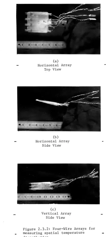
The two basic probe configurations are pictured in figure 2.3.2.
Depending upon requirements the vertical or horizontal array is used in
coniunction with the appropriate traversing equipment (figure 2.3.3) to
determine the approximate instantaneous spatial temperature field. Once
the choice of probe array is made it is secured to the probe holder,
whose main purpose besides connecting the probe to the traverse shaft is
to constrain the individual probes to a constant vertical position
be-tween the plates. The upper and lower teflon runners are spring loaded
and ride at all times on the aluminum plates. The probe leads themselves
are plugged into a special female connector mounted at the end of the
D.C.
BRIDGE
NETWORK
GALVANOMETER
Figure 2.3.1: The constant current bridge network used for
31. (a) Horizontal Array Top View (b) Horizontal Array Side View (c) Vertical Array Side View
Figure 2.3.2: Four-Wire Arrays for measuring spatial temperature distribution
32.
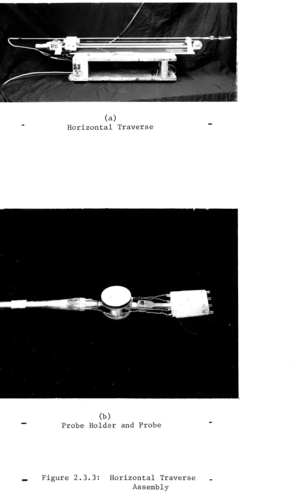
(a)
Horizontal Traverse
(b)
Probe Holder and Probe
Figure 2.3.3: Horizontal Traverse . Assembly
and exit at the rear. The shaft is secured to a carriage that rides
on linear bearings along a pair of 1.59 cm precision stainless steel
shafts. The carriage is driven as shown by a PIC positive drive belt
that is geared to a variable D.C. motor. The position of the carriage,
which can run a total of 63.5 cm, is monitored by the voltage output of
a linear 2K ohm voltage divider connected to the drive gear train. The
speed can be varied from 9 to 45 cm/sec. Before each traverse the probe
and probe holder are enclosed in a plexiglass guide shown in figure 2.3.4
(much like a cattle chute) complete with a sliding door that can be open
just prior to injection into the convection tank. This use of the door
keeps room disturbance of the interior flow field to a minimum.
Because the stationary probe has a greater tendency to disturb the
flow the wires are mounted somewhat differently than on the moving probes.
Instead of the sewing needles, the unetched sections of the Wollaston
wire, to either side of a small etched section in the middle, are the
supports for the etched section that serves as the probe. The- silver
ends are soldered to leads at the lower end of the probe tubing. These
sections are interchangable and are passed through the probe guide in the
upper section and plugged into an upp~er section which is attached
perma-nently to the lift plate of the vertical traverse (figure 2.3.5). The
34.
(a)
(b)
-Figure 2.3.4: Horizontal Traverse -Chute
VERTICAL TRAVERSE
o - potentiometer
b -probe holdef C - drive screw
d - drive motor
Figure 2.3.5: Traverse for measuring vorftical temperature gradients and
36.
CHAPTER III
METHODS AND PROCEDURES OF DATA COLLECTION
3.1 Basic Gap Measurements
One of the versatile features of the apparatus is the potential
variability of the plate separation. However care must be taken in
or-der to ensure (a) a maintenance of parallel plates and (b) an accurate
measurement of the separation.
The first requirement can be assured by floating the lower plate assembly in molten cerrobend and aligning the upper plate with the lower.
The three threaded supports equally spaced around the outer edge of the
upper thermal bath, the sag adjustment screw in the center, and three
gauge blocks equally spaced on a circle of one half tank radius are used
to establish the parallelism of the plates. It is fcund that if the
cool-ing rate of the cerrobend is slow enough (i.e. 80*C to 30"C in more than 20 hours) there is no detectable distortion in the parallel plate
separa-tion.
Accurate measurement of the plate separation is indeed important
be-cause of the cubic dependence of the Rayleigh number on this measurement.
A depth micrometer that is inserted through the vertical probe guide into the tank is used to measure the separation of the plates in different
configurations. Using this method one is able to determine the relative
plate separation to within + .001 by sighting along the upper or lower
plate through a plexiglass port in the outer wall of the tank. Use is
the plate as either the gap or the temperature difference between the
plates -is changed.
3.2 Temperature Measurements
Great care was taken in determining the temperatures of the three
plates. At the outset two representative thermocouples of each batch of
chromel-constantan wire were chosen for calibration. The emf versus
temperature characteristics of well constructed thermocouples only vary
according to the wire compositions. The couples were placed in a
well-stirred vacuum bottle of water with a small heater and a Parr precision
thermometer and were monitored through the same switching system that is
used for the plate temperature measurements. The K-3 potentiometer
mea-sured the emf of each couple with respect to an ice point that is
con-stant + .005*C, as the temperature of the water was increased from 10*C to 80*C in increments of about 3-40C.
Originally it was thought that each plate temperature could be
de-termined from an average emf reading of the thermocouple. This could be
done by wiring the couples of each separate plate in series or parallel.
However individual thermocouples short circuit to the aluminum plate
oc-casionally and the ground loops that result degrade the accuracy of the
other attached thermocouples. So for the experiments to be discussed
each of the thermocouples on a radius of the individual plates was
moni-tored and recorded. Consequently the temperature distribution of the
plates under varying conditions is well documented. In this manner
38.
distribution of the plates under isothermal conditions near room
tem-perature. Differences in emf output varied by less than.l yv (.0164*C)
over 30.5 cm of a radius.
3.3 Temperature Fluctuation Measurements
Of course the most interesting temperature measurements are those made of the spatial temperature field of the air between the two plates.
Most of these measurements were done with the resistance wire probes,
although the slower responding thermocouples were used to measure mean
vertical temperature gradients in a non-convecting tank.
Again it was found that, just as in the case of the thermocouples,
wire composition and geometry are the factors that affect the
sensitivi-ty of the wire resistance to a temperature change. So the extensive
calibrations were performed on three rake arrays constructed from the
same wollastan wire reel. These arrays were secured to a jig and placed
in a specially constructed isothermal tank. The individual wire
resis-tances as measured on the bridges shown in figure 2.3.1 were compared to
the outputs of thermocouples also located on the jig as the temperature
was changed. Comparison of the results for each wire shows that the
tem-perature sensitivities of equal length wires is the same and that only
a datum resistance for each individual wire has to be determined before
each series of measurements. In practice this datum is found by
insert-ing the particular array of interest into the convection tank under
iso-thermal conditions and noting Lhe resistance of each wire. Various
occurred from trial to trial. These changes can be attributed to the
variations of contact resistance of the pins on the array leads. The
measured sensitivity of the wires remained constant.
Three point calibrations covering the working temperature range
were made for each of the stationary probes by placing the probes into
an isothermal tank for three different temperatures. The stationary
probes using thermocouples are easier to use than the resistance probes
because the calibration is made only once and they are far more durable.
Their slower time response restricts their use to measurement of the
tem-perature distribution of stably stratified air.
3.4 Heat Flux Experiments
The heat flux-Rayleigh number relationship and the accompanying
slope discontinuities were the focus of the first investigation in our
apparatus. Because Rayleigh number can be changed by variation of either
plate separation or temperature difference independently, both types of
heat flux experiments were conducted. It has already been mentioned that
the dimensionless heat flux is defined in terms of the Nusselt number.
The nature of the Nusselt number, a ratio of total heat flux to
conduct-ive heat flux, requires a knowledge.of the conductconduct-ive heat flux of this
particular apparatus. Therefore, a series of experiments on both a stably
and unstably stratified air layer was carried out.
There were various heat flux calibration problems including both
radiation heat transfer and sidewall heat loss that are treated in detail
40.
of the range of AT2 and plate separation. Two general sets of
experi-ments were conducted to determine heat flux. In early experiexperi-ments
we-assumed that the lower plate temperature had to be maintained close to
the cerrobend melting point so that parallax could be avoided.
Conse-quently a series of experiments with a constant lower plate temperature
(63.30C) were performed. -For a later series of heat flux experiments it was found that slow cooling over a 24 hour period would cause no tilt in the lower plate. Therefore the second set of heat flux measurements
were performed with the mean temperature of the convection tank at 25*C.
All experiments were performed under steady state conditions
com-pared to the slowly varying experiments of W. & D. (1967b) and Malkus.
The criterion for steady-state that evolved is related to the steadiness
of the temperature difference across the glass plate as the heat flux
adjusts to the new boundary conditions after Ra-change. Experience has
indicated that the differential output from the thermocouples on either
side of the glass plate would typically oscillate + .75 pv (the limit of
the resolution capabilities of the K-3 potentiometer) under "steady-state"
conditions. Therefore all measurements are made at least thirty minutes
after changes in this output become smaller than those limits.
The stated goal of this phase of the investigations was to
esta-blish the validity and nature of the slope changes in the heat flux
be-havior. Series of experiments that ranged over the apprcpriate Rayleigh
numbers were run for both independent changes in AT 13 2 or the plate separa-tion. W. & D. (1967b) define heat flux regimes corresponding to the
(iii) 8000<Ra<24,000, and (iv) 24,000<Ra<52,000. The incremental changes
in either h or AT2 necessary for the successive observational points
were calculated from the ten equally spaced Ra in each of the above
re-gions. Experimental series in which Ra was
varied by changing only AT2
(fixed h) were conducted for different plate separations. This type of
series will be referred to henceforth as a
SAT
2-series, while itscounter-part will be referred to as a 6h-series. In order to complete a partial
coverage of the possible AT 2-h combinations 6h--series were performed for
a few different AT2 's
This range of temperature differences and plate separations was
covered for both stable and unstable temperature distributions.
Esti-mates of the heat loss at the sidewall are inferred from the temperature
measurements on either side of the plexiglass-styrofoam sidewall.
With the confirmation of the various breaks in the heat flux curve
a more detailed study of the transition region was undertaken. It was
necessary to determine the acuteness of the break and whether there is
any hysteresis associated with these features of heat flux change. The
results of these various tests will be discussed th-oroughly in section
4.4.
3.5 Temperature Distribution Experiments
The resistance wire probe and the horizontal traverse, described
in Chapter II, were used to gather temperature distribution information
from the air convecting heat between the plates. The block diagram in
informa-DATA
COLLECTION
Figure 3.5.1: Experimental system for measuring...
temperature fluctuations
tion. A major concern in this type of investigation is the disturbance
of the flow one is trying to investigate. It is important that the probe
does not distort the flow before the temperature measurement is made.
Three steps were taken in order to minimize the possibility of disturbing
the flow by the probe. As figure 2.3.3 shows the very thin rake array
is supported 7 cm ahead of the major flow disturbing element of the probe
assembly. The effectiveness of this geometry was tested by passing the
moving array within millimeters of a stationary probe. Resulting
distur-bances came well after the moving probe had passed by. In one accidental
case a stationary wire showed no disturbance before it was broken by the
moving probe.
The door, pictured in figure 2.3.4 at the entrance to the convection
tank, remained closed during the time intervals between measurements
made by the rake array. Thirdly long tima intervals were allowed
be-tween successive probe injections.
The criterion used for determining the time lapse between runs is
related to the time scales of the adjustment of the mean convective
flow field to finite amplitude perturbations. In the physical geometry
considered the horizontal length scale is necessarily the most
signifi--cant when determining the transmission of flow disturbances throughout
the flow field. For low Ra near critical Chen and Whitehead (1967) have
shown the importance of the diffusion time scales. Because the Prandtl
number is close to 1, the viscous and thermal diffusion time scales are
comparable and either scale is probably applicable for small Ra where
44.
time scale is related to the quantity, Nr , where T = mean orbital period of a roll and N is the number of rolls. For conditions of the
experiments presented here, a characteristic orbital velocity of 1.5
cm/sec (an average orbital period of 5.5 sec) can be estimated from the
two-dimensional numerical results of Chorin (1966) for Pr = 1 (N = 20, h
= 2 cm). So typical horizontal time scales are in the order of 2 minutes
for Ra > 10 . As a result of this estimate it is felt that the ten minute wait allowed five time constants for the influence of the probe
wake to diffuse. Indeed successive runs separated by more than 5 min-4
utes showed no systematic influence on each other for Ra > 10 . Results were not quite as convincing for lower Ra so minimum periods of twenty
minutes were used between trials. The first measurement of the
tempera-ture at each new Ra made in a tank that had been undisturbed for more
than two hours and sometimes up to twelve hours.
The smoke visualization of rolls by W. & D. (1970) for Ra < 2x10⁴ is convincing evidence that rolls are the main convection element for
those Ra. The main objective of this investigation is to define the
de-tailed physical changes in the flow as the slope changes in the heat
flux curve are traversed. Different aspects of the flow are studied using
the two different types of probes discussed previously. The horizontal
array supplies details about (i) the wavelength characteristics of the
roll structure as well as (ii) the relative roll orientation. Variations
in the vertical modal structure of the flow field are detected by the
vertical array. The coordinated use of the injected arrays and one or
significance of certain characteristics of the temporal response of
stationary temperature probes reported by other investigators (such as
Townsend, 1959). Because this apparatus can accomodate at least two
stationary probes at any height in the tank simultaneously, variable
point correlation studies are possible. Furthermore the speed
adjust-ment capabilities of the tape recorder allow one to make very long time
runs necessary to obtain statistical significance from temporal
tempera-ture fluctuation data.
After individual series of temperature measurements by each type
of array, it was decided that the horizontal array would provide the most
informative data of the instantaneous temperature field. The discussion
in a later section will reveal in more detail how the vertical array has
shown very little variation of structure in the vertical temperature
per-turbation structure for Ra < 50,000. At least for Ra < 20,000 it is evident that the changes in horizontal modal structure are responsible
for the major increase in convective heat transfer. Consequently the
horizontal array was used extensively for the studies in that range.
A typical series of temperature fluctuaticn runs presented in de-tail in Chapter V is the result of a primary interest in the Rayleigh
numbers that approach the transition Rayleigh numbers from above and
be-low. The plate separation for a particular
SAT
2-series is usually chosen so that the maximum temperature difference AT2 occurred at the highestRa of interest. We were restricted by the size of the probe that allowed a minimum plate separation of 1.5 cm. Table 3.1 summarizes the different series of temperature fluctuation measureim.ents. The i-3entification of
TABLE 3.1
Summary of Experimental Conditions for'Temperature Fluctuation Runs Series Identifica-tion Array Non I.D.
bimensional
Height Mean Temp. (*C) AT2-Change Range h (0C) (cm) h-Change Range AT 2 (cm) (OC) TF-I III (HF-XXXV) IV (HF-XXXVII) V (HF-XLITT) VII (HF-XLIV) VIII (HF-XLV) A-1 A-2 A-1 A-1 A-1 A-1 A-1 A-2 various Ti, .05 .25 .20 .28 60-45 60-45 5-37 5-37 2.01 2.01 25 5-19.5 1.95 25 5-27.06 2.73 25 9.1-23.9 1.67 changing changing changing 1.575-1.73 4.3-24.5 4.3-24.5 3.9-13.9 9.8-53.4 4.0-12.85 21.0 7.93-10.64 1.6-3.03 20.3 1.4-6.05 7.3-54 .11-760 Horizontal Array Vertical Array Ra x 10 Range A-1 = A-2 =simultaneous heat flux measurements is made in the parentheses below
the identification of the temperature fluctuation run. Deardorff and
Willis' (1967) observations of maximum spatial temperature variance.had
an influence on the height at which temperature measurements were made.
As a result of preliminary analyses of the temperature fluctuations
mea-sured at Ra < 50,00 a final series of runs probing the mean temperature boundary layer was made for Ra = 0 (105). The vertical array was chosen to further investigate the evolution and role of three-dimensional
struc-tures observed intermittently at the lower Ra. Because of the vertical
penetration of these "plumes" in the flow at lower Ra, it was felt that
their growth most likely originated in the boundary layer. For TF-VIII,
Ra was varied by changing plate separation because (i) Ra in this range
can only be attained with large plate separation and (ii) the spacing of
the vertical probes changes very little with respect to the mean
bound-ary layer scale with an increase in Ra in this way. The reasons for
48.
CHAPTER IV
RESULTS OF HEAT FLUX MEASUREMENTS 4.1 Rayleigh Number Determination
Most comparisons made betwecn the different results of this and
other experiments are based on the value of Ra, and of course Pr which
is relatively fixed for one fluid. It is especially important when
comparing features of convection at low Ra that the calculation of Ra
be discussed.
Since the quantities
4Z
and V are temperature dependent, an average value (i.e. that associated with the mean tank temperature)is used for the calculation. In this case their values are determined
from a linear interpolation of the values in table 4.1.1.
Tem
Table 4.1.1.
Kinematic viscosity and thermal diffusivity of dry air at sea level. (National Bureau of Standard Circular 564)
2 2 p (*C) c x 10) c x 10) Pr 2 s1e.c 9. sec 23.3 9.50 . 13.18 .72 26.7 76.6 15.90 20.80 22.20 29.81 .71 .69
V
0 6 8Because these values can vary as
much
as 5% from source to source there could be confusion in comparing the resulLs of different authors.tempera-ture because air is assumed to be a perfect gas.
Both the plate separation, h, and the unstable temperature
dif-ference between the two plates,
A
T^, are measured quantities and 4contribute the major part of the error in the determination of Ra.
It can be shown that if the random errors associated with
measure-ment are Gaussian, the percentage error in Ra in relation to the
percentage error in each of the quantities that compose it in the
following way,
2.-where \Af v4 &T and
w
are the absolute uncertaintiesof each of the respective quantities. It is quite evident how the
percentage error in the h-measurement is the major source of Ra error
and should be discussed. The percentage error in the values of
physi-cal parameters is an order of magnitude less than the least of the
other errors.
For thermal convection between horizontal plates one sometimes
compares the results of the experiment to a model where the governing
parameters are constant throughout the flow field for a particular set
of boundary conditions. It is important on one hand to know how
accu-rately the parameters are determined from experiment to experiment,
while a knowledge of the variability of the parameters throughout the
flow field is also important.
It is discussed- in sections 3.1 and 3.2 ho. the actual h andAT
50.
measurements are made. The luncertainty in the average h determination
is the sum of the possible measurement error and the estimated
variation of plate separation. The estimate of the uncertainty in
h is less than .0125 cm which means that the percentage error in h
will be less than 1.25% for plate separations greater than 1cm. There
is a + .03*C scatter associated with the linear segments that
approxi-mate the thermocouple calculation curve. Because this calibration is
not linear over the range of temperature differences commonly used
in these experiments, differential thermocouple measurements were not
used. Therefore, a doubled error of + .06*C accompanies each
A
T 2 determination. Therefore, except for 3uch experimental configurationswith the combined effect of AT 2> 25*C and h<lcm, the uncertainty in Ra is less than 4%. It is a rare experiment performed in this
apparatus that di not satisfy the restrictions above.
The variation of Ra in the convection tank itself can be
attri-buted to the combination of plate tilt and waviness and the effects
of the radical temperature gradients in both the upper and lower
plates. Relative waviness and tilt of the plates is at most .0045cm.
The same uncertainty in the control of plate sag adds to the waviness
error to yield a worst-case error
for h_>1
of .9%. Because the tem-perature difference between the plates has a mean temtem-perature closeto room temperature (&25*C), the radial gradients in the plates are
proportional to their respective difference with the room temperature.
80% of the plate surface, to the temperature difference, AT2, is quite nearly constant for all temperature difference between the
plates. The ratio less than .0015 for AT 2s is greater than 5*C.
In general there was no convection for AT2 < 5*C in these
experi-ments. Therefore for the restrictions states above the worst case
variation of Ra will be less than 3%. Since most of the temperature
fluctuation observations are made with h--2cm and 100C <T
2
<
300C,the errors will be considerably less than those upper bounds above.
Of course the errors discussed so far do not account for syste-matic uncertainties such as property value error or incorrect
thermo-couple calibration. However, we are quite confident that any
syte-matic errors in these measurements must be quite small because of the
accuracy with which the heat flux data predicts the critical Ra.
Figure 4.1.1 shows the data of two different heat flux series plotted
with the results presented by Silveston (1958). To the precision with
which Ra can be measured the data imply the critical Ra Ra cr=1720, which agrees well with the prediction of the Ra for the onset of
.4
1.5
Figure 4.1.1:
2.0
RA
x
10~
Heat Flux Results Near Racr
a - Silveston (water) + - XXIV 3 - XLIV
1.2
1. 1
1.0
0.9
0.8
3.0
04.2 Heat Flux Calculations
This section describes how heat fluxes are determined from the
measurements of temperature difference,
A
T, across the glass platefor a variety of conditions. Due to the asymmetry of the apparatus
the usual procedure of measuring the temperature difference across
symmetric heat flux layers, top and bottom, was inapplicable. For
these heat flux calculations the dependence of
A
T1 on isdetermined in the conduction regime (sub-critical Ra) and extrapolated'
into the convection regime. (See any of the data for three separate
series presented in figures 4.1, 2 & 3).
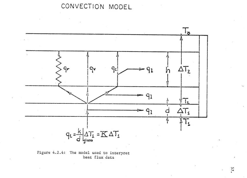
The basis for this type of treatment is examined in the
follo-wing model. From figure 4.2.4 we see that the follofollo-wing simplified
heat flux balance can be made,
(4.2.1)
where TT T - T 1 1 2'
It heat flux through the glass plate;
C = heat flux due to conduction that reaches upper plate; v = heat flux due to fluid motion - convection;
-r heat flux due to radiation; generalized heat flux loss; and
-Z = heat meter "conatant".
1. 6
.5-
.4-
.3-
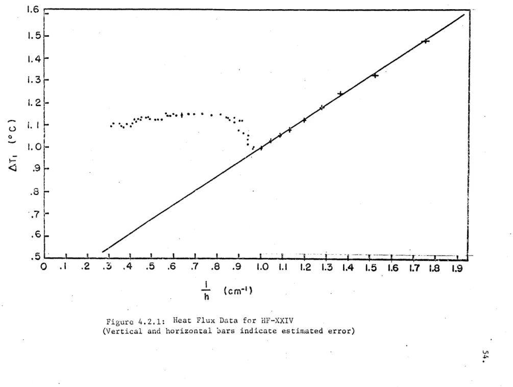
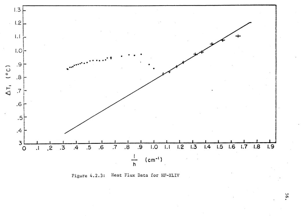
I.2-. - -.. 4 .5 .6 .7 .8 .9 1.0 1.1 1.2 1.3 1.4 1.5 1.6 1.7 1.8 1.9:
I~oh
IC
n
Figure 4.2.1: Heat Flux Data for HF-XXIV
,*..-- -O , . *. I I I p I I I I I I
0
.1
.2
.3
.4
.5
.6
.7
.8
.9
.
1.1
1.2
1.3
1.4
1.5 1.6
1.7
1.8
h
1.9
(
cm~'
)
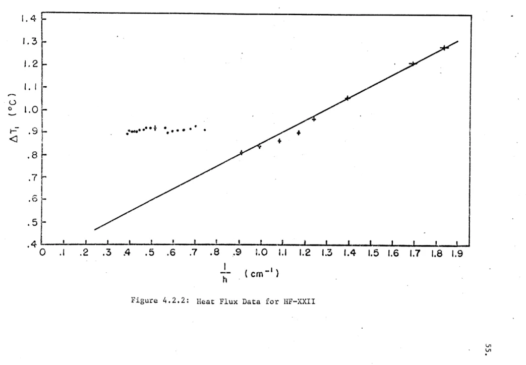
Figure 4.2.2: Heat Flux Data for HF-XXII
1.3
1.2
1.1
-
1.0-.8
.7
61-.
3
F
I.2V
I.8
.4
O0
I
,
3
.
.
6
.
8
.
1.0
1.1
1.2
1.3
1.4
1.
5 1.
6 1.7 .1.8
1.9
(cm-')
~~A~T
=]KA7T
9
c*+
Figure 4.2.4: The model used to interpret heat flux data
58.
The heat meter "constant", under ideal conditions with both perfect
insolation and temperature measurements, would be a constant ratio of
the thermal conductivity of glass and the plate thickness, d. In this
case we have relaxed this constraint in order to compensate for heat
losses and measurement inaccuracies.
If we specifically consider the conduction (or sub-critical
re-gime) we note v= 0 and that
(4.2.2)
where T is that part of the temperature difference associated with
-10
conduction alone. It is found experimentally, for the ranges of AT, 4 and h considered, that 'land are proportional to A T2 so that
(4.2.2) can be rewritten as,
(4.2.3)
where I = C . AT 2/h. For the case where
A
T is held constant4 c . air 2 2
and h is varied in order to change Ra, the quantity, (C +C )A 2 is
constant and the slope, S, of a A T - 1/h plot is inversely
pro-portional to